The spectral flow for Dirac operators on compact planar domains with local boundary conditions

Let $H$ be a complex separable Hilbert space, $\left(A_{t}\right)$, $t\in[0,1]$ be a continuous 1-parameter family of bounded self-adjoint (or, what is the same, Hermitian) Fredholm operators in $H$. Near zero every $A_{t}$ has discrete real spectrum, which changes continuously with the variation of $t$. Hence one can count the net number of eigenvalues of $A_{t}$ passing through zero in positive direction as $t$ runs from $0$ to $1$, that is, the difference between the numbers of eigenvalues (counting multiplicities) crossing zero in positive and negative directions. This net number is called the spectral flow $\spf\,(A_{t})$. The description of this notion can be found in [2, 3].

The case when $A_{0}$ or $A_{1}$ has zero eigenvalue requires some agreement on the counting procedure; we use the following convention: take a small $\varepsilon>0$ such that $A_{0}$, $A_{1}$ have no eigenvalues in the interval $[-\varepsilon,0)$, and define the spectral flow as the net number of eigenvalues of $A_{t}+\varepsilon I$ which pass through zero.

Let now $\left(A_{t}\right)$ be an 1-parameter family of (not necessarily bounded) self-adjoint Fredholm operators in $H$. For example, it can be a family of symmetric elliptic differential operators $A_{t}$ acting on sections of Hermitian bundle $E$ over closed (that is, compact without boundary) manifold $X$. The definition of the spectral flow can be adjusted to this case, though more accurate consideration is needed, particularly due to the presence of various natural topologies on the space of such operators [4, 5, 6].

When a manifold has non-empty boundary, we have to consider the family $\left(A_{t},B_{t}\right)$, where $A_{t}$ is a formally self-adjoint differential operator, and $B_{t}$ is a “good” (self-adjoint elliptic) boundary condition for $A_{t}$ at any $t$. One can see the notion of self-adjoint elliptic boundary value problem for operators of Dirac type in [3, 7], and for general first order elliptic operators in [8].

Such differential operator $A_{t}$ with boundary condition $B_{t}$ defines the unbounded self-adjoint Fredholm operator on $L^{2}(X,E)$, which has unbounded discrete real spectrum. Intuitively, the spectrum of $\left(A_{t},B_{t}\right)$ changes continuously with the variation of $t$, so the definition of the spectral flow works in this case as well [4, 6]. However, the proof that the definition and the standard properties of the spectral flow are correct is considerably more difficult in this case. The crucial ingredient is the continuity (in $t$) of the family $\left(A_{t},B_{t}\right)$ in the space of unbounded self-adjoint Fredholm operators on $L^{2}(X,E)$ with an appropriate metric. This was proved in [8] (see [8], Theorem 7.16). This continuity property allows one to use the theory developed in [4, 5] in full force. Our proof of Theorem 3 (see Part II) crucially depends on this theory, and, in particular, on Theorem 7.16 from [8]. The results of this theory needed for the proof of Theorem 3 are isolated in Section 11 as properties (P0-P4).

Note that if the spectra of $(A_{0},B_{0})$ and $(A_{1},B_{1})$ are the same (isospectral operators), which is the case in this paper, then there is another way to define the spectral flow of $(A_{t},B_{t})$. The set

can be uniquely represented as the union of the graphs of functions $\lambda_{i}(t)$ such that $\lambda_{i}(t)\leqslant\lambda_{j}(t)$ for $i\leqslant j$. These functions give us the bijection (one-to-one correspondence) of the spectrum of $(A_{0},B_{0})$ to the spectrum of $(A_{1},B_{1})$. If these spectra coincide as subsets of $\mathbb{R}$ then this correspondence gives us the shift of the spectrum on the integer number of positions. This number is the spectral flow of $(A_{t},B_{t})$. It is worth to note that for the isospectral case one can replace the level $\lambda=0$ by any real number, and the difference between eigenvalues crossing the level in positive and negative directions will be the same [2].

Suppose $X$ is a compact planar domain bounded by $m$ smooth curves (topologically it is a disk with $m-1$ holes). We will use the notations $x=(x^{1},x^{2})\in X$, $\partial_{i}=\partial/{\partial x^{i}}$.

Let us consider the Dirac operator on $X$

acting on a spinor function $u\colon X\to\mathbb{C}^{2}$, $u=\begin{pmatrix}u^{+}\\ u^{-}\end{pmatrix}$.

A Dirac operator with non-zero vector potential has the form

$q$ is a smooth function from $X$ to $\mathbb{C}$.

Let $\mu\colon X\to U(1)$ be a gauge transformation; we suppose that $\mu(x)\in\mathbb{C}$, $|\mu(x)|\equiv 1$ for $x\in X$. Let us take a Dirac operator $D_{0}=\mathbb{D}+Q_{0}(x)$ and connect it with the conjugate operator

by an one-parameter family of Dirac operators

$q_{t}$ is a smooth function from $X$ to $\mathbb{C}$ continuously depending on $t$, $t\in[0,1]$,

A self-adjoint locally elliptic²² 2 Another name for “locally elliptic boundary condition” is “Sapiro-Lopatinskii boundary condition” local boundary condition for $D_{t}$ has the form

where $B\colon\partial X\to\mathbb{R}\setminus\left\{0\right\}$ is a smooth function defining the boundary condition, $n=\left(n_{1},n_{2}\right)$ is the outward conormal to the boundary $\partial X$ of $X$ at point $x$, and we identify $n$ with the complex number $n_{1}+in_{2}$ in (3).

Note that $n_{1}$, $n_{2}$ coincide with the components of the outward normal to $\partial X$ for the case of Euclidean metric considered both here and in the next section. In Section 5 we consider a more general case of arbitrary metric on $X$, and the distinction between a normal and a conormal becomes essential there.

Boundary condition (3) is gauge invariant with respect to the conjugation by $\mu$, while $D_{0}$ and $D_{1}$ are conjugate by $\mu$. So the operators $D_{0}$, $D_{1}$ with the same boundary condition (3) are isospectral, and the spectral flow of the family $D_{t}$ gives us the shift of the spectrum of $D_{t}$ when $t$ runs from $0$ to $1$.

Note that since $B\neq 0$, it has definite sign at each boundary component $\partial X_{j}$, so the constants $b_{j}$ are correctly defined. The restriction of $\mu$ to $j$-th connected component of $\partial X$ gives us the map from the circle $\partial X_{j}$ to the circle $U(1)$; $\mu_{j}$ is the degree of this map.

This theorem follows from more general result which we formulate below. The generalization goes in two directions: (1) we allow arbitrary dimension of unknown complex functions $u^{-}$, $u^{+}$, (2) we replace Dirac operator by operators of more general form. The value of $c_{2}$ is computed in Section 6.

Let $X$ be as in the previous section. The standard $2N$-dimensional Dirac operator has the form

$I_{N}$ is $N\times N$ unit matrix.

We will consider operators of the form $D=\mathbb{D}+Q(x)$ acting on spinor functions

where $Q$ is a smooth map from $X$ to the space $\mathsf{H}(\mathbb{C}^{2N})$ of complex self-adjoint (or, what is the same, Hermitian) $2N\times 2N$ matrices.

A self-adjoint local elliptic boundary condition for the operator $\mathbb{D}+Q$ has the form

where $B$ is a smooth map from $\partial X$ to the space of complex self-adjoint invertible $N\times N$ matrices, $n=\left(n_{1},n_{2}\right)$ is the outward conormal to $\partial X$ at point $x$, and we identify $n$ with the complex number $n_{1}+in_{2}$.

The equivalent way of imposing boundary condition (6) is

This result is the corollary of Theorem 3 from the following section.

Let $X$ be a compact planar domain bounded by $m$ smooth curves and equipped with a Riemannian metric $g$ (which is not necessarily flat).

We call a first order formally self-adjoint operator $D$ over $X$ a Dirac type operator if its symbol has the form

where $\Phi$ is a smooth map from $X$ to the group $\GL^{+}(2,\mathbb{R})$ of real invertible $2\times 2$ matrices with positive determinant, and the matrices $\sigma_{1}$, $\sigma_{2}$ are defined by formula (4).

In other words, Dirac type operator is the operator acting on spinor functions (5) and having the following form:

where $Q$ is a smooth map from $X$ to the space $\mathsf{H}(\mathbb{C}^{2N})$ of complex self-adjoint $2N\times 2N$ matrices,

(superscript $t$ denotes the operation of taking the formal adjoint operator). More explicitely,

where $\sqrt{g}=\sqrt{det(g_{ij})}$, the matrix $(g_{ij})$ is inverse to the matrix $(g^{ij})=(\left\langle dx^{i},dx^{j}\right\rangle_{g})$, $\sqrt{g}\;dx^{1}dx^{2}$ is the volume element on $X$ (of course, $g_{ij}$, $g^{ij}$, and $\sqrt{g}$ depend on $x$).

By $\mathcal{D}=\mathcal{D}_{X,\,g,\,N}$ we denote the space of all operators having the form (9) for fixed $X$, $g$, $N$. Note that Dirac type operator (that is an element of $\mathcal{D}_{X,\,g,\,N}$) is uniquely defined by the pair $(\Phi,Q)$.

A self-adjoint elliptic local boundary condition for Dirac type operator (9) has the form

where $B$ is a smooth map from $\partial X$ to the space of complex self-adjoint invertible $N\times N$ matrices, the complex-valued function $n^{\prime}$ on $\partial X$ is defined by the formula $n^{\prime}=n^{\prime}_{1}+in^{\prime}_{2}$ with $(n^{\prime}_{1},n^{\prime}_{2})=(n_{1},n_{2})\Phi$ and $n=(n_{1},n_{2})$ being the outward conormal to $\partial X$ at $x\in\partial X$. Recall that $n_{i}=\sum g_{ij}n^{j}$ for the components $\left(n^{j}\right)$ of the normal to the boundary.

By $\mathcal{B}=\mathcal{B}_{X,\,N}$ we denote the space of all smooth maps from $\partial X$ to the space of complex self-adjoint invertible $N\times N$ matrices.

Suppose $D\in\mathcal{D}$, $B\in\mathcal{B}$. We will write $(D,B)$ for operator (9) acting on the domain

where $C^{1}(X,\mathbb{C}^{2N})$ is the space of continuously differentiable functions from $X$ to $\mathbb{C}^{2N}$.

Such operators have the following properties:

1. 1.

   For any $D\in\mathcal{D}$, $B\in\mathcal{B}$ the operator $(D,B)$ is (unbounded) essentially self-adjoint Fredholm operator, which has the discrete real spectrum. All its eigenvectors are smooth functions. (Lemma 1, Section 10)

2. 2.

   Suppose $Q_{t}(x)$ is continuous on $(t,x)$, $D\in\mathcal{D}$, $B\in\mathcal{B}$. Then all the operators from the family $\left(D+Q_{t},B\right)$ have the same domain, and this family is norm continuous in $L^{2}\left(X,g;\mathbb{C}^{2N}\right)$. Therefore the spectral flow of the operators family $\left(D+Q_{t},B\right)$ is well defined ([5], Proposition 2.2).

Now we can formulate the main result of the present paper:

Note that constant $c_{m}$ in all the Theorems 1-3 is the same.

Here we compute the spectral flow for the case when $X$ has just one hole ($m=2$), and as a result find $c_{2}$.

If $\lambda_{j}(t)$ are the continuous functions from the interval $[0,1]$ to $\mathbb{R}$ such that $\Lambda\cap\left\{0\leqslant t\leqslant 1\right\}$ is the union of the graphs of functions $\lambda_{j}(t)$ and $\lambda_{i}(t)\leqslant\lambda_{j}(t)$ for $i\leqslant j$, then $\lambda_{j}(t)=j+t$ when $-3\leqslant j\leqslant 2$ (up to shift of the numeration). So

On the other hand, by Theorem 3,

where by $\partial X_{1}$, $\partial X_{2}$ we denote the inner and the outer boundary circles respectively. Therefore $c_{2}=1$.

In this section we provide some evidence supporting the conjecture that $c_{m}=1$ for all $m$.

Namely, let us realize $X=X^{h}$ as $(m-1)$ identical annuli arranged along the line and connected by the band of the width $h$, with the corners smoothed out, as on the Fig. 2.

Let us consider the process of continuous decreasing of the band’s width from $h=1$ to $h=0$; we suppose that the annuli do not change in progress. Let us fix some function $\mu$ from $X^{1}$ to $U(1)$ and take $q_{t}=it\mu^{-1}\left(\partial_{1}\mu+i\partial_{2}\mu\right)$. Restricting $\mu$ and $q_{t}$ on $X^{h}$, $0<h\leqslant 1$, we obtain operator (2) over $X^{h}$. Let us define the boundary condition by $B^{h}=+1$ at the inner part $\cup_{j<m}\partial X^{h}_{j}$ of $\partial X^{h}$ and $B^{h}=-1$ at the outer part $\partial X^{h}_{m}$ of $\partial X^{h}$.

By Theorem 1, $\spf\,(\mathbb{D}+Q_{t})=c_{m}\sum_{j<m}\mu_{j}$ does not depend on $h$. It is natural to suggest that the limit at $h\to+0$ of the (constant) spectral flow of the family $\left(\mathbb{D}+Q_{t},B^{h}\right)$ for $X^{h}$ is equal to the spectral flow of $\left(\mathbb{D}+Q_{t},B^{0}\right)$ for the “limit” domain $X^{0}$, which is the disjoint union of $m-1$ annuli, and the “limit” boundary condition $B^{0}=+1$ at the inner boundary and $B^{0}=-1$ at the outer boundary of every annulus.

However, $\spf\,(\mathbb{D}+Q_{t},B^{0})$ for such union is the sum of $\spf\,(\mathbb{D}+Q_{t},B^{0})$ for the annuli, and hence is equal to $\sum_{j<m}c_{2}\mu_{j}=c_{2}\sum_{j<m}\mu_{j}$.

Therefore, if the assumption on the limit behavior of the spectral flow is true, then $c_{m}=c_{2}$ at any $m>2$.

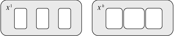
Another way to have a look at the general case is to fix the outer boundary and to increase the holes up to their merging, as on Fig. 3. Here we obtain the single annulus in the limit of $h=0$, and the same result $c_{m}=1$ if the passage to the limit will be justified.

Alternatively, we can combine these two methods to obtain arbitrary number $m^{\prime}$, $1\leqslant m^{\prime}\leqslant m-1$ of annuli in the end of the limit process, with the same result for $c_{m}$.

The results of the present paper are concerned only with the case when $X$ is a disk with holes. Easy modification of the proof gives us analogue of this result for the case of smooth compact oriented surface $X$ with nonempty boundary, with the only change of $c_{m}$ to $c_{m,\,g}$, where $c_{m,\,g}$ is the integer constant depending on the number $m$ of boundary components of $X$ and on the genus $g$ of $X$. However, this still remains within the very restricted framework: all the operators $D_{t}$ are of Dirac type, both symbol of $D_{t}$ and boundary condition do not depend on $t$, conjugating gauge transformation is scalar.

In fact, this result can be extended to much more general case. Namely, let $X$ be a smooth compact surface, $(A_{t})$ be an 1-parameter family of first order symmetric elliptic differential operators acting on sections of unitary vector bundle $E$ over $X$, and subbundle $L_{t}$ of $\left.E\right|_{\partial X}$ defines a self-adjoint elliptic local boundary condition for $A_{t}$ at any $t$. Suppose that $(A_{1},L_{1})$ is conjugate to $(A_{0},L_{0})$ by some gauge transformation $\mu$ (that is $\mu$ is unitary isomorphism of $E$, not necessarily scalar). Then operators $(A_{1},L_{1})$, $(A_{0},L_{0})$ are isospectral, and there arises the natural question about the spectral flow of the family $(A_{t},L_{t})$. This question will be considered in a forthcoming paper by the author [10]. In that paper we will prove that

where $c_{m,\,g}$ is the integer depending on the number $m$ of boundary components of $X$ and on the genus $g$ of $X$, $\varphi_{j}$ is the integer determined in a canonical way by the restrictions on $j$-th boundary component of the following data:

1. (1)

   family $(\rho_{t})$, where $\rho_{t}$ is the symbol of $A_{t}$;

2. (2)

   family $(L_{t})$ of boundary conditions;

3. (3)

   gauge transformation $\mu$.

In particular, the spectral flow of $(A_{t},L_{t})$ does not depend on the choice of the operators in the interior of $X$ but only on the symbol of the operators on the boundary.

Theorem 3 of present paper fits into this general result as follows: $c_{m}=c_{m,\,0}$, $\varphi_{j}=b_{j}\mu_{j}$. Recall that $\mu_{j}$ is invariant of the restriction of $\mu$ to $j$-th boundary component of $X$, $b_{j}$ is defined from the restrictions of boundary condition and of the operator’s symbol on $j$-th boundary component.

In this section we compare our boundary condition (6) with “the general boundary conditions for the Dirac equation” for 4-dimensional Dirac operators formulated by Akhmerov and Beenakker in [1]. After that, we give some computations for the spectral flow in terms of [1]. In particular, we show that the spectral flow vanishes in the case of time reversal symmetry (under the assumption of local ellipticity of the boundary problem).

In this section we will temporarily use the notations from [1] in their original form and will formulate our results in the same terms.

The long-wavelength and low-energy electronic excitations in graphene considered in [1] are described by the Dirac equation $H\Psi=\varepsilon\Psi$ with Hamiltonian

acting on a four-component spinor wave function $\Psi=(\Psi_{A},\Psi_{B})$ (in our notations, $\Psi$ is two-dimensional spinor function, $\Psi_{A}=u^{+}$, $\Psi_{B}=u^{-}$, $N=2$). Here $v$ is the Fermi velocity, $\bm{p}=-i\hbar\nabla$ is the momentum operator, $\bm{\sigma}\cdot\bm{p}=-i\hbar\left(\sigma_{1}\nabla_{1}+\sigma_{2}\nabla_{2}\right)$, matrices $\tau_{i},\sigma_{i}$ are Pauli matrices in valley space and sublattice space, respectively:

References

- [1] A. R. Akhmerov and C. W. J. Beenakker. Boundary conditions for Dirac fermions on a terminated honeycomb lattice. Phys. Rev. B 77 (2008) 085423; arXiv:0710.2723v3 [cond-mat.mes-hall]
- [2] M. F. Atiyah, V. K. Patodi, and I. M. Singer. Spectral asymmetry and Riemannian geometry. III. Math. Proceedings of the Cambridge Philosophical Society 79, part 1 (1976) 71.
- [3] B. Booss-Bavnbek, K. P. Wojciechhowski. Elliptic Boundary Problems for Dirac Operators, Birkhauser, 1993.
- [4] B. Booss-Bavnbek, M. Lesch, and J. Phillips. Unbounded Fredholm Operators and Spectral Flow. Canad. J. Math. 57 (2005) 225; arXiv:math/0108014v3 [math.FA]
- [5] M. Lesch. The uniqueness of the spectral flow on spaces of unbounded self-adjoint Fredholm operators. In: Spectral geometry of manifolds with boundary and decomposition of manifolds (B. Booss-Bavnbek, G. Grubb, and K.P. Wojciechowski, eds.), Cont. Math., vol. 366, Amer. Math. Soc., 2005, pp. 193-224; arXiv:math.FA/0401411
- [6] B. Booss-Bavnbek, M. Lesch, and J. Phillips. Spectral Flow of Paths of Self-Adjoint Fredholm Operators. Nucl. Phys. B Proceedings Supplement 104 (2002), 177.
- [7] J. Bruning and M. Lesch. On boundary value problems for Dirac type operators: I. Regularity and self-adjointness. Funct. Anal. 185 (2001) 1; arXiv:math/9905181v2 [math.FA]
- [8] B. Booss-Bavnbek, M. Lesch, and C. Zhu. The Calderon Projection: New Definition and Applications. J. of Geometry and Physics 59 (2009), No. 7, 784; arXiv:0803.4160v3 [math.DG]
- [9] M. V. Berry and R. J. Mondragon. Neutrino billiards: time-reversal symmetry-breaking without magnetic fields. Proc. R. Soc. London, Ser. A 412 (1987) 53.
- [10] M.F. Prokhorova. The spectral flow for first order elliptic operators on a compact surface. In preparation.
- [11] R. S. Strichartz. Multipliers on fractional Sobolev spaces. J. of Mathematics and Mechanics, 1967. Vol. 16, No. 9, pp. 1031-1060.
- [12] W. Fulton, J. Harris. Representation theory. A first course. Graduate Texts in Mathematics, Readings in Mathematics, 129. Springer-Verlag, 1991.
Ural Federal University, Ekaterinburg, Russia
pmf@imm.uran.ru