A Complementarity Partition Theorem for Multifold Conic Systems

Assume $K\subseteq{\rm I\!R}^{n}$ is a closed convex cone and $A\in{\rm I\!R}^{m\times n}$. Consider the homogeneous conic system

and its alternative system

where $K^{*}\in{\rm I\!R}^{n}$ is the dual of $K^{*}$. It is immediate that any solutions $\bar{x}$ and $\bar{y}$ to (P) and (D) respectively are complementary, that is, they satisfy $\bar{y}^{\rm T}(A\bar{x})=0$. In particular, if either (P) or (D) has a strict feasible solution, then the other one only has trivial solutions. In the special case when $K={\rm I\!R}^{n}_{+}$, a stronger related property holds. As a consequence of Goldman-Tucker Theorem [3], there always exist solutions $\bar{x}$ and $\bar{y}$ to (P) and (D) respectively such that $\bar{x}+A^{\rm T}\bar{y}\in{\rm I\!R}^{n}_{++}$. Such pairs of strictly complementary solutions are associated to a canonical partition $B\cup N=\{1,\dots,n\}$ of the index set $\{1,\dots,n\}$ (see Proposition 1 below). The partition sets $B$ and $N$ correspond to the most interior solutions to (P) and (D) respectively. Furthermore, there is a nice geometric interpretation of the sets $B,N$ (see Proposition 2 below).

We present a generalization of the above strict complementary results to more general conic systems. To that end, we consider the case when the cone $K$ is the direct product of $r$ lower-dimensional regular closed convex cones. That is, we assume

where $K_{i}\subseteq{\rm I\!R}^{n_{i}}$ is a regular closed convex cone for $i=1,\dots,r.$ Throughout the sequel we shall use $I$ to denote the set $I=\{1,\dots,r\}$ and $n$ to denote the dimension $n=\sum_{i=1}^{r}n_{i}$.

Following the terminology introduced in [2] we call the conic systems (P) and (D) multifold when the cone $K$ is as in (1). This type of multifold structure is common in optimization. Formulations for linear programming (LP), second-order conic programming (SOCP) and semidefinite programming (SDP) problems generally lead to feasibility problems of this form. Our first main result (Theorem 1) shows that there are some canonical subsets $B,N$ and $B_{0},N_{0}$ of $I$ associated to certain geometric properties of the problems (P) and (D). These sets generalize the partition sets $B,N$ in the case $K={\rm I\!R}^{n}_{+}$. Our second main result (Theorem 2) shows that there exists a unique canonical partition of the index set $I$ associated to the most interior solutions to (P) and (D).

The paper is organized as follows. Section 2 provides the foundation for our work, namely the existence of strictly complementary solutions to (P), (D) when $K={\rm I\!R}^{n}_{+}$. Section 3 presents our main results, namely Theorem 1 and Theorem 2. Section 4 discusses in more detail the special case of second-order conic systems. Section 5 concludes the paper with some final remarks.

To motivate and state our main results, we first consider the special case when $K={\rm I\!R}^{n}_{+}$ in (P), (D). In this case the conic systems become

and

where $A\in{\rm I\!R}^{m\times n}$. This can be considered as a special case of a multifold conic system with $r=n$ and $K_{i}={\rm I\!R}_{+}$ in (1). Hence throughout this section we have $I=\{1,\dots,n\}$. Furthermore, for notational convenience, we shall write $A=\begin{bmatrix}a_{1}&\cdots&a_{n}\end{bmatrix}\in{\rm I\!R}^{m\times n}$. In other words, $a_{i}\in{\rm I\!R}^{n}$ is the $i$-th column of $A$. The following result is a consequence of the Goldman-Tucker Theorem for linear programming [3].

The partition sets $B,N$ in Proposition 1 can be described is several ways. The three descriptions of $B,N$ displayed in Proposition 2 below lay the foundation for our main work. In the sequel we use the following convenient notation. For a convex cone $C\subseteq{\rm I\!R}^{d},$ let ${\rm Lin\,}(C)\subseteq{\rm I\!R}^{d}$ denote the lineality space of $C$, that is, the largest linear subspace contained in $C$. Observe that because $C$ is a convex cone, ${\rm Lin\,}(C)=\{x\,|\,x,-x\in C\}.$

The description (6) of the sets $B,N$ has an interestcolorreding geometric interpretation. What determines if a particular index $i$ belongs to $B$ or $N$ is whether the corresponding $i$-th column $a_{i}$ lies in the lineality space of the cone $A{\rm I\!R}^{n}_{+}$. This geometric interpretation has an interesting extension to multifold conic systems as Theorem 1 below shows. Proposition 2 is a consequence of Farkas Lemma and is also a special case of Theorem 1 below.

Consider now the general conic systems (P), (D) where $A\in{\rm I\!R}^{m\times n}$ and the cone $K\subseteq{\rm I\!R}^{n}$ is as in (1). For notational convenience, write $A=\begin{bmatrix}A_{1}&\cdots&A_{r}\end{bmatrix}$, where $A_{i}\in{\rm I\!R}^{m\times n_{i}}$ is the $i$-th block of the matrix $A$.

Our main results generalize Proposition 1 and Proposition 2 to multifold conic systems. Motivated by (4), define

Likewise, motivated by (5), define

We are now ready to state our main results. The following theorem establishes a characterization of the index sets $B,B_{0},N,N_{0}$ in terms of the geometry of the sets $AK$ and $A_{i}K_{i}$. In the statement below, $\overline{AK}$ denotes the closure of $AK$.

To ease exposition, we defer the proof of Theorem 1 to the end of this Section.

Observe that in the case when $K$ is a polyhedral cone, we have $AK=\overline{AK}$. Thus for $K$ polyhedral Theorem 1 yields $B=B_{0}$ and $N=N_{0}$. In particular Proposition 2 readily follows from Theorem 1.

The next theorem generalizes Proposition 1. It shows that there is a unique canonical partition of the index set $I$ into six complementarity subsets of indices.

The Venn diagram representing the relations between the subsets of $B$, $B^{\prime}$, $N$, $N^{\prime}$, $C$ and $O$ of $I$ is given in Fig. 1.

In Section 5.1 we provide an example of a second-order conic programming problem for which all six sets are nonempty. It should be noted that a six-set partition for second-order conic programs similar to the one suggested here was mentioned in [1, Section 6]. However, there was no prior characterization of this partition along the lines of Theorem 1.

We conclude this section with the proof of Theorem 1. Our proof relies on the following separation lemma. Although this result is likely known, we were not able to locate it in the literature in this exact form.

Consider the special case when the cone $K$ in (P),(D) is a cartesian product of Lorentz cones. In other words,

where

Here $\|\cdot\|$ is the Euclidean norm in ${\rm I\!R}^{n_{i}}.$ We shall put, by convention, $\mathcal{L}_{0}={\rm I\!R}_{+}$ when $n_{i}=1$. Also, for $d\geq 1$ we will let ${\rm I\!B}_{d}\subseteq{\rm I\!R}^{d}$ denote the Euclidean closed unit ball in ${\rm I\!R}^{d}$ centered at zero.

For each $i\in I$ assume the $i$-th block $A_{i}\in{\rm I\!R}^{m\times n_{i}}$ of $A$ is of the form

In other words, $A_{i0}$ denotes the first column of $A_{i}$, and $\bar{A}_{i}$ denotes the block of remaining $n_{i}-1$ columns. Put

Observe that $AK={\rm cone\,}\mathop{\rm co\,}_{i\in I}\{E_{i}\}.$ Theorem 1 can now be stated in a way that more closely resembles (6) in Proposition 2.

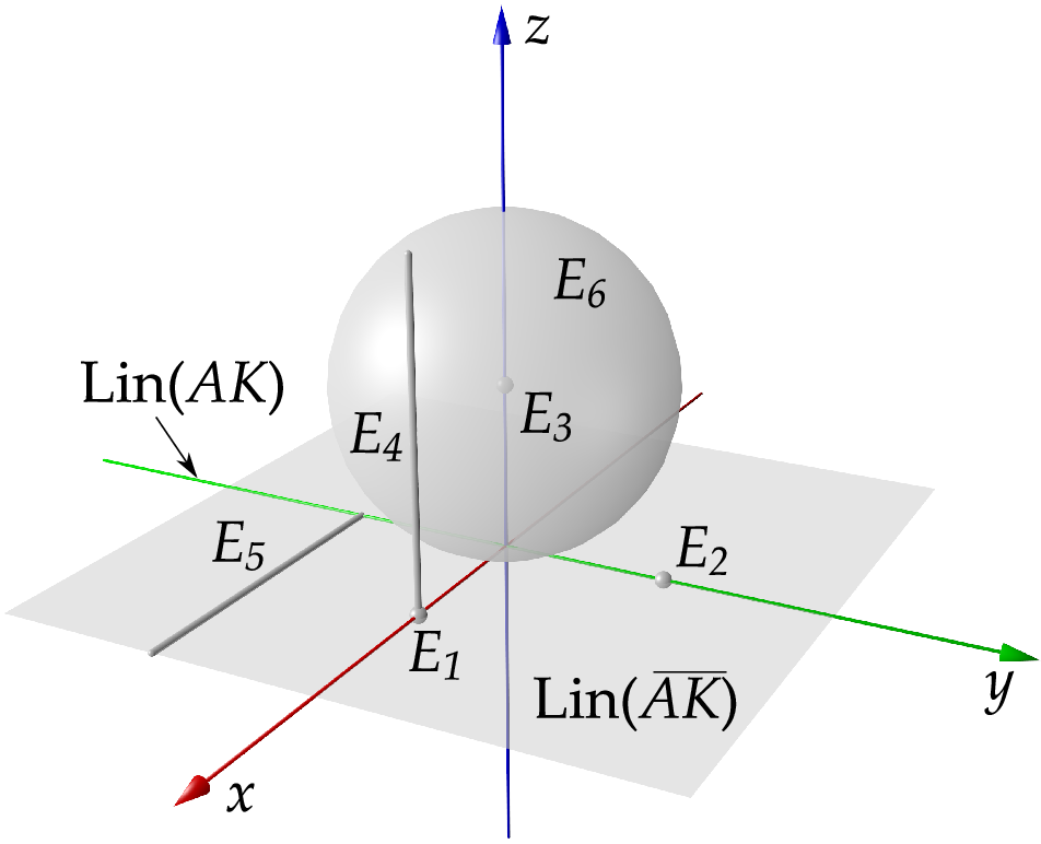
We now discuss an example of a second-order feasibility system where all six sets $B,N,B^{\prime},N^{\prime},C,O$ in the partition of Theorem 2 are nonempty.

References

• [1] F Alizadeh and D Goldfarb. Second-order cone programming. Math. Progr. Ser. B, 95(1):3–51, 2003.
• [2] D. Cheung, F. Cucker, and J. Peña. A condition number for multifold conic systems. SIAM J. Optim., 19(1):261–280, 2008.
• [3] A.J. Goldman and A.W. Tucker. Theory of linear programming. Linear Inequalities and Related Systems, H.W. Kuhn and A.W. Tucker (eds.), Annals of Mathematical Studies, 38:53–97, 1956.
• [4] J.-B. Hiriart-Urruty and C. Lemaréchal. Fundamentals of Convex Analysis. Springer-Verlag, Berlin, 2001.