Rich-club network topology to minimize synchronization cost due to phase difference among frequency-synchronized oscillators

We first define synchronization cost due to phase difference in an unweighted and undirected network which is described by an adjacency matrix $A$ and consists of $N$ phase oscillators. $A_{ij}$ is $1$ when oscillators $i$ and $j$ are connected, and $A_{ij}$ is $0$ when they are not. According to the Kuramoto model, the phase of the oscillator $i$, $\theta_{i}$, is described as

where $\omega_{i}$ is the natural frequency of the oscillator $i$, and $\epsilon$ is a coupling strength. To reduce computational cost for the following rewiring-based optimization, we assume that $\epsilon$ is constant for any combination of oscillators. In this Kuramoto model, the synchronization cost between oscillators $i$ and $j$, $S_{ij}$ is defined based on the phase difference between the connected oscillators as follows:

Note that the synchronization cost is only defined after the network of the oscillators reaches to a state of frequency synchronization. As described in Appendix A, in power grids, $S_{ij}$ can be regarded as an index that is proportional to power loss due to difference in voltage phase between power plants $i$ and $j$.

Based on the definition of $S_{ij}$, we numerically estimate $S_{ij}$ for each edge in the following four steps for a given network:

1. (i)

   We set normally-distributed $\{\omega_{i}\}$ for each node. It is because that previous studies on real networks such as power grids and brain networks have assumed that the natural frequencies of belonging oscillators are symmetrically fluctuating around the averaged frequency [29, 22, 4].

2. (ii)

   Based on the Kuramoto model described in Eq. (1), we numerically estimate frequency-synchronized status, where $\dot{\theta_{i}}$ becomes a common constant value, $\Omega$, for any $i$.

3. (iii)

   In the frequency-synchronized status, each oscillator has a different specific phase, $\theta_{i}$. Based on the set of $\{\theta_{i}\}$, we then evaluate $S_{ij}$ for each edge.

4. (iv)

   As described in (i), the set of the natural frequency, $\{\omega_{i}\}$, is fluctuating over time. Thus, the $S_{ij}$ is also fluctuating over time. Therefore, we repeat the procedure (i)-(iii) 200 times with different sets of $\{\omega_{i}\}$, and obtain 200 different sets of $\{S_{ij}\}$. Then, we average the $\{S_{ij}\}$ over time, obtaining $\left<S_{ij}\right>$ for each edge. Finally, we average the $\left<S_{ij}\right>$ across edges, and obtain $\left<S\right>$ for the entire network.

To search for the optimal network topology with the least $\left<S\right>$, we adopt the rewiring method that previous studies used to explore the network topology with the largest synchronizability [25]. We apply the following rewiring-based optimization procedure to a given connected network with $N$ nodes and mean degree of $\left<k\right>$: At each step, the number of rewired edges is randomly determined based on an exponential distribution. The set of edges to be rewired is also randomly chosen in a given network. After the rewiring, we estimate frequency-synchronized status and obtain $\left<S\right>_{\rm updated}$. The attempted rewiring is rejected if the updated network is disconnected. Otherwise, the rewiring is accepted if $\Delta\left<S\right>=\left<S\right>_{\rm updated}-\left<S\right>_{\rm initial}<0$, or with probability $p=\min(1,[1-(1-q)\Delta\left<S\right>/T]^{1/(1-q)})$ where $T$ is a temperature-like parameter and $q=-3$ [25]. The initial rewiring is conducted at $T=\infty$, and, after the first $N$ rewiring, $T$ is set as $(1-q)(\Delta\left<S\right>)_{\max}$ where $(\Delta\left<S\right>)_{\max}$ is the largest $\Delta\left<S\right>$ in the first $N$ rewiring trials. After that, $T$ is decreased $10\%$ in every $10$ rewiring trials. This estimation process iterated until there is no change in more than 50 successive rewiring steps. We apply this rewiring-based optimization to three different initial networks: an Erdős-Rényi (ER) random model, Watts-Strogatz (WS) model [30], and a Barabási-Albert (BA) model [31] with $N=50$ and $\left<k\right>=4$ [25]. In all the cases, the coupling strength, $\epsilon$, is set to be $0.3$. Each set of the natural frequencies of Kuramoto oscillators, $\{\omega_{i}\}$, is randomly chosen from the normal distribution with an average of $100\pi$ and a standard deviation of $1$.

During the optimization, we trace the standard order parameter, $r$, and local synchoronizability, $r_{\rm local}$ [32], defined as follows:

where $N_{l}$ is the total number of edges, $\Gamma_{i}$ is the set of neighbors of node $i$, and $\psi$ is a global phase. Furthermore, after the optimization is completed, we compare the optimized networks from the different initial networks by estimating the following basic topological properties: mean of shortest path length [33], mean of clustering coefficient [30], mean of betweenness centrality [34], and degree correlation [34]. We conducted ten optimizations of ten different networks for each type of the initial networks, and averaged these basic properties.

• •

  The shortest path length, $\ell_{ij}$, is defined as the shortest distance between two nodes $i$ and $j$ [33]. The averaged shortest path length, $\left<\ell\right>$, is defined as the average value of $\ell_{ij}$ over all the possible pairs of nodes in the network.

• •

  The clustering coefficient for node $i$, $C_{i}$, measures the local group cohesiveness [30], which is defined as the ratio of the number of links between the neighbors of $i$ and the maximum number of such links. We define the mean clustering coefficient, $\left<C\right>$, as an average value over all the nodes.

• •

  The betweenness centrality for node $i$, $b_{i}$, is defined as the number of shortest paths between pairs of nodes that pass through a given node [34]. We define the mean betweenness centrality, $\left<b\right>$, as an average value over all the nodes.

• •

  The degree correlation for a network is defined as the Pearson assortativity coefficient of the degrees, $r_{\rm assortative}$ [34]. The coefficient enables us to quantify the preference for high-degree nodes to attach to other high-degree nodes. Networks with this preference show large $r_{\rm assortative}$.

We estimate reich-club coefficient, $\Phi(k)$, for both initial networks and optimized networks. According to the previous studies [26, 27, 24, 28], the coefficient for each degree $k$ is calculated as

where $E_{>k}$ represents the number of edges among $N_{>k}$ nodes that have more than $k$ degrees. As in previous studies [27, 24, 28], we calculate normalized rich-club coefficients, $\Phi_{\rm norm}(k)$ through dividing the raw value, $\Phi(k)$, by the mean of rich-club coefficients of 100 random networks (ER models), $\Phi_{\rm random}(k)$, as follows,

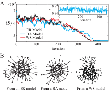
Fig. 1 shows representative results of the rewiring-based optimizations. $\left<S\right>$ was decreased from approximately $6.5\times 10^{-2}$ to $4.5\times 10^{-2}$ even when the initial network structure was different. In all the initial networks, $\left<S\right>$ reached to a stable status after approximate 400 steps of rewiring. Strikingly speaking, we cannot guarantee that the optimal network was found, but this result suggests that a reasonably robust approximation of the optimal topology was obtained in this method.

During the optimization, the standard order parameter, $r$, were fluctuating just below 1 during the optimization (a small panel in Fig. 1 A). The local synchonizability, $r_{\rm local}$, showed the similar fluctuation below 1. Considering the previous studies on these parameters [32], these behaviors of $r$ and $r_{\rm local}$ are considered to be related to the amount of the coupling strength, $\epsilon$. The previous studies [32] have demonstrated that, when the coupling strength is more than 0.2, both of $r$ and $r_{\rm local}$ reach a plateau that is near to 1 regardless of network topology. In the present study, the coupling strength, $\epsilon$, was set at 0.3, because global synchronization is necessary for the estimation of $\left<S\right>$. This relatively large coupling strength could result in the saturation of the global and local order parameters, $r$ and $r_{\rm local}$ during the optimization process.

Fig. 1 B shows that the optimized networks for the three different initial networks commonly exhibit a characteristic topology, which has a densely interconnected core nodes and peripheral nodes dangling the core module. The heterogeneous network features were also observed in the basic network properties in the optimized networks (Tab. 1). Compared with the initial networks, the optimized networks tended to show larger averaged values of the shortest path length, $\left<\ell\right>$, betweenness centrality, $\left<b\right>$, and degree correlation, $r_{\rm assortative}$. The averaged values of the clustering coefficients, $\left<C\right>$, were smaller in the optimized networks. These results suggest that, through the optimization process, the network seems to enlarge its heterogeneity.

This heterogeneous network topology has been reported as ”rich-club” organization in a series of previous theoretical and experimental studies [26, 27, 24, 28]. The prior literatures have characterized the organization by estimating normalized rich-club coefficients, $\Phi_{\rm norm}(k)$ described in Eq. 6. If the network has rich-club organization, $\Phi_{\rm norm}(k)$ should be more than $1$, and increase monotonically as $k$ increases.

Fig. 2 shows the comparison in $\Phi_{\rm norm}(k)$ between initial networks and optimized networks. To clarify the difference in the rich-club coefficients, we adopted as the initial networks larger networks than shown in Fig. 1 B (i.e., $N=100,\left<k\right>=4$). Before the optimization, $\Phi_{\rm norm}(k)$ was not always larger than $1$ (e.g., ER and WS models), and did not show monotonic increase along $k$, which is consistent with a previous study [27]. In contrast, in the optimized networks, the rich-club coefficients were larger than $1$ in almost all the range of $k$, and monotonically increased as $k$ increased. These phenomena were observed commonly among the three different optimized networks that were derived from the three different initial networks. In addition to the appearance of the networks in Fig. 1 B, this estimation of $\Phi_{\rm norm}(k)$ supports the notion that the networks with rich-club organization has the minimum or a very small amount of synchronization cost due to phase difference among frequency-synchronized oscillators.

As shown in Fig. 1 B, the rich-club network topology consists of high-degree nodes cluster and low-degree peripheral nodes. Therefore, we hypothesized that the topology can be characterized by a bimodal degree distribution. To test the hypothesis, we estimated Wolfson’s polarization index, $\hat{P}$ [35]. The Wolfson’s index for degree distribution is defined as:

where $\left<k\right>$ is the mean of the degree, $k_{i}$, and $m$ denotes the median of the degree. $\left<k\right>_{1}$ and $\left<k\right>_{2}$ are the mean values of $\{k_{i}\bigm|k_{i}<m\}$ and of $\{k_{i}\bigm|k_{i}\geq m\}$, respectively. $G$ represents Gini inequality index, which is defined as $G=\frac{1}{2\left<k\right>}\sum_{i=1}^{N}\sum_{j=1}^{N}\bigm|k_{i}-k_{j}\bigm|$. This Wolfson’s polarization index shows the extent of the bimodality of the distribution. If the distribution is completely the same as a uniform distribution, the $\hat{P}$ is $0$. If the half of population has nothing and the other half shares everything, the $\hat{P}$ reaches a maximum, $0.25$. In the present case, a larger $\hat{P}$ indicates that the network has a more bimodal and bipolarized degree distribution.

We estimated $\hat{P}$ during the rewiring-based optimization. Because $\hat{P}$ can be calculated more accurately for networks with more nodes, we used the BA model with $N=100$ and $\left<k\right>=4$ as an initial network for the optimization. As a result, in the course of the above-mentioned optimization, $\left<S\right>$ decreased during the rewiring-based optimization (Fig. 3A). Meanwhile, as $\left<S\right>$ decreases, $\hat{P}$ increases (Fig. 3B). Actually, the degree distribution changed from a power-law distribution (Fig. 3C) to a bimodal distribution (Fig. 3D). This relation was also observed for different initial networks (e.g., ER model). This correlation supports the hypothesis that rich-club network with small $\left<S\right>$ can be characterized by its bimodal degree distribution.

We finally provide an analytical interpretation on why the rich-club network has less $\left<S\right>$. Using mean-field approximation, the Eq. (1) in the frequency-synchronized status can be described as $\Omega=\omega_{i}-\epsilon k_{i}\sin(\theta_{i}-\psi)$, where $\psi$ is defined in the Eq.  (3). Therefore, if $|\theta_{i}-\psi|$ is small enough, $\theta_{i}-\psi=\frac{1}{\epsilon k_{i}}(\omega_{i}-\Omega)$, and $(\theta_{i}-\theta_{j})^{2}$ is described as

for a set of $\{\omega_{i}\}$. $\left<S_{ij}\right>$ is obtained as averaged $(\theta_{i}-\theta_{j})^{2}$ across an enough number of sets of $\{\omega_{i}\}$. As in the above-described numerical estimation, we assume that $\{\omega_{i}\}$ is distributed according to the normal distribution with a mean of $\omega_{0}$ and a standard deviation of $\sigma$, and that the synchronized frequency is always $\Omega$ in every set of $\{\omega_{i}\}$. Because we can also assume that $\omega_{0}$ is nearly equal to $\Omega$, $\left<(\omega_{i}-\Omega)^{2}\right>$ is considered to be equal to $\sigma^{2}$, and $\left<(\omega_{i}-\Omega)(\omega_{j}-\Omega)\right>$ is considered to be equal to zero. Consequently, we obtain the approximation of $\left<S_{ij}\right>$ as follows:

This approximation was validated through comparison of $\tilde{\left<S_{ij}\right>}$ with the real $\left<S_{ij}\right>$, as shown in Fig. 4 A ($\sigma=1,\epsilon=0.3$). The two parameters had a large negative value of Pearson’s correlation coefficient ($-0.88$).

This expression of $\tilde{\left<S_{ij}\right>}$ gives qualitative explanation on relationship between rich-club network topology and a small value of $\left<S\right>$: To achieve a small amount of $\left<S\right>$, $\tilde{\left<S_{ij}\right>}$ should be small. When the node $i$ has a high degree, it makes more contribution to a smaller $\tilde{\left<S_{ij}\right>}$ to connect with a the node $j$ with a high degree. It is also case when the node $i$ has a small degree. As a result, for a small value of $\tilde{\left<S_{ij}\right>}$, high degree nodes should connect with other high degree nodes, and low degree nodes should not have edges with other low degree nodes, but with high degree nodes. Consequently, high degree nodes tend to be gathered and create a densely-connected core module, and low degree nodes tend to connect with high degree nodes in the core module. Overall, the optimized network with a small amount of $\left<S\right>$ is likely to be a rich-club network.

Note that it is difficult to further extend this approximation. If this approximation of $\left<S_{ij}\right>$ is accurate enough, a simple calculation of Eq. 9 leads us to the proportional relationship between $\left<S\right>$ and $\frac{1}{\left<k\right>}\left<\frac{1}{k}\right>$. Given $\left<k\right>$ is a constant value as in the present study, $\left<S\right>$ should be proportional to $\left<\frac{1}{k}\right>$. However, as shown in Fig. 4 B, we could not observe a linear relationship. This inaccurate approximation of $\left<S\right>$ may be caused by accumulation of the small difference between $\left<S_{ij}\right>$ and $\tilde{\left<S_{ij}\right>}$. This result suggests that we cannot extend this approximation to represent $\left<S\right>$ only by $\left<\frac{1}{k}\right>$.