Account of Nuclear Scattering at Volume Reflection
Abstract
For a particle traversing a bent crystal in the regime of volume reflection we evaluate the probability of interaction with atomic nuclei. Regardless of the continuous potential shape, this probability is found to differ from the corresponding value in an amorphous target by an amount proportional to the crystal bending radius, and the particle deflection angle. Based on this result, we evaluate the rate of inelastic nuclear interactions, and the final beam angular dispersion due to multiple Coulomb scattering. The theoretical predictions are compared with the experiments. The impact of multiple Coulomb scattering on the mean volume reflection angle is also discussed.
Keywords:
bent crystal; volume reflection; inelastic nuclear interactions; multiple Coulomb scatteringpacs
61.85.+p, 29.27.-a, 45.10.-bI Introduction
Deflection of fast charged particle beams by bent crystals is a developing branch of accelerator technology, pursuing the goal of steering ultra-high energy beams in a restricted laboratory space. Till the last decade, the conventionally exploited deflection mechanism in bent crystal tools was channeling [1], but an alternative promising technique based on volume reflection [2] has emerged recently, dealing with over-barrier particles, and offering the benefit of large angular acceptance (equal to the crystal total bending angle) and almost 100% deflection efficiency. Some drawback of the volume reflection technique is the smallness of the deflection angle, which is of the order of Lindhard’s critical angle , with the planar potential well depth, and the particle energy. This angle is independent of the crystal thickness, but a buildup of the deflection angle can nonetheless be acheived by transmitting the particle through a sequence of bent crystals [3], or arranging a composite volume reflection from several atomic planes in one crystal [4]. An additional advantage of the volume reflection mechanism is that it applies equally well to negative particles, for which channeling is spoiled by the unavoidable multiple Coulomb scattering on atomic nuclei residing at the bottom of the potential well.
The origin of the volume reflection effect is essentially dynamical, due to non-linearity of the motion in the strong continuous potential of bent atomic planes. At that, incoherent scattering effects on individual atomic nuclei can be held small compared to the deflection angle mean value. That even admits using for volume reflection experiments the crystals of thickness mm, which by times exceeds the volume reflection region extent, estimated as [5].11 1 At typical beam energy GeV (CERN SPS) entailing rad, and at optimal radius m, this longitudinal scale amounts to mm. However, in other respects, for instance for evaluation of the deflected beam angular spread, the multiple Coulomb scattering can not be ignored. Worth mentioning also are the inelastic nuclear interactions, which can be registered as multiple secondary particle signals in the beam loss monitors. Such events are relatively rare, and therefore present no danger for the primary beam propagation, but from their rate one can determine the robustness of the volume reflection inside the crystal. In fact, since physically they occur due to interaction with the same nuclei as Coulomb scattering, the rates of these processes must be closely related. Similar processes also include atomic K-shell ionization and the accompanying characteristic X-ray radiation occurring at fast charged particle passage close to an atomic nucleus.
Outside the volume reflection area, we know that the particle motion becomes highly over-barrier, whereby the rate of fast particle scattering on atomic nuclei must approach that in an amorphous medium. Thus, in the thick-crystal limit, the number of nuclear interactions in the whole crystal roughly equals that in an amorphous target of same material and thickness. But that kind of approximation is unsuitable if the crystal thickness is comparable with the volume reflection area extent, or if one aims to exploit the nuclear interactions, for monitoring the in-depth particle dynamics. Since the number of nuclear interactions in an amorphous medium, is known precisely enough from various experiments, it may be neatly subtracted and in this way the difference be measured. Yet the theory interpreting this difference needs to be developed.
For a consistent treatment of incoherent multiple scattering at volume reflection, one needs to solve the kinetic equation in a non-uniform external field, but in general that does not seem feasible by analytic means. Still, there must exist a domain in which the Coulomb scattering is sufficiently small for perturbative account, and there are reasons to expect it to cover the practically interesting range of beam and crystal parameters where most of the presently available data belong.
The aim of the present paper is to evaluate the rate of nuclear interactions adhering to the framework of the perturbative approach. Given the 1d (radial) character of volume reflection dynamics in the pure continuous potential of a uniformly bent crystal, the corresponding particle trajectories may be expressed analytically, and the probability of a nuclear interaction be calculated along the known path. In Sec. II we implement this procedure, for particles of different charge sign, and different orientations of the crystal: (110) and (111). In Sec. III limitations of the perturbative approach are determined. In Sec. IV we apply the results of Sec. II to the probability of inelastic nuclear interactions at specific experimental conditions, comparing the theory with the experiment. In Sec. V we extend the theory predictions to elastic scattering and address the issue of the volume-reflected beam angular divergence. The conclusions are given in Sec. VI.
II Inelastic nuclear interaction probability under neglect of Coulomb scattering
Volume reflection process assumes particle interaction with the bent crystal in a planar orientation. At that, the atomic density in each plane may be regarded as uniform. Since all the nuclei are located in the planes, one particle crossing of an atomic plane may be viewed as an elementary act of nuclear interaction. If all the planes are packed them with the same density and equidistant22 2 For a silicon crystal, that corresponds to planar orientaton (110), which is most frequently used in experiments on volume reflection. Another used case is planar orientation (111), involving 2 non-equidistant planes within the period. Extension to that case is straightforward and will be considered later in this section., with the inter-planar distance , the probability of any kind of nuclear interaction in one atomic plane crossed at a tangential angle is
| (1) |
where is the corresponding cross-section on a single nucleus, and the atomic density in the crystal volume. For elastic scattering one must employ the transport cross-section (), while for inelastic interactions – the total inelastic cross-section on a Silicon nucleus (). More specifically, the inelastic interactions may be genuinely nuclear, involving multiple hadron production, or electromagnetic, e.g., ionization of the small-radius atomic K-shell33 3 For silicon (), the atomic K-shell radius is , which is quite small compared to the interplanar distance . To knock out a K-shell electron, a relativistic charged particle must pass at a distance from the electron yet much smaller than . Thus, to ionize the K-shell, the charged particle has to pass through a really close vicinity of the atomic nucleus, and in this respect the process is similar to a nuclear interaction. and the accompanying characteristic X-ray radiation. In the Glauber approximation, all the high-energy nuclear and electromagnetic cross-sections are energy-independent, though one might take their weak energy dependence into account, if desired.
In the case of a straight crystal, and for a highly over-barrier particle, when is much greater than the critical value,
| (2) |
and thus is subject to negligible variation within the crystal , summing up contributions (1) for crossed planes would yield the total nuclear interaction probability:
| (3) |
This value is independent of and , and is equal to the corresponding probability in an amorphous medium – not surprisingly since the particle flow covers each nucleus with the same density, equal to that in the initial beam outside the crystal. In this sense, one can speak about an “amorphous orientation” of a perfect crystal even. By the same token, the latter notion applies in bent crystal regions where the particle motion is highly over-barrier.
In the volume reflection case, however, condition (2) in the vicinity of a radial reflection point breaks down. In this region the plane crossing angle varies considerably along the particle path, hence it is to be evaluated accurately at each plane crossing. To this end, the particle trajectory must be computed beyond the straight line approximation and, neglecting the multiple scattering, we are going to approximate it by a trajectory in the pure continuous potential. If the crystal is bent uniformly (which is sufficiently credible nowadays), the trajectory description simplifies in cylindrical coordinates, with the bent planes corresponding to surfaces of constant radius relative to some axis far outside of the crystal. Thereat, the plane crossing angle sine entering Eq. (1) expresses simply as the time derivative of the particle radial coordinate:
| (4) |
Inserting Eq. (4) to Eq. (1) and summing over all the planes crossed by the particle, we obtain the total inelastic nuclear interaction probability in a bent crystal:
| (5) |
Since the particle motion straightens out away from the volume reflection area, there the nuclear interaction rate per unit length should approach that in an amorphous medium. Hence, the difference between the number of nuclear interactions in an oriented crystal and in an “unoriented” crystal may be expressed as
| (6) |
where the isolated geometrical factor
| (7) |
is expected to be finite and independent of , representing the excess (or deficit) of the target nuclear interaction range.
In this section we will concentrate on evaluation of limit (7). To begin with, note that the trajectory in a centrally-symmetric continuous potential is symmetric with respect to the reflection point, enabling one to count the crossed planes beginning from the reflection point in only one direction and double the result:
| (8) |
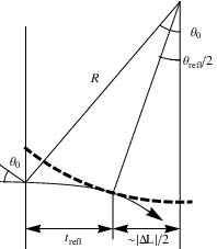
Here is the distance from the reflection point to the crystal boundary – say, its front face, where the entrance angle relative to the atomic planes is known (see Fig. 1). This quantity is expressible through the particle trajectory, too. In fact, at large it is unambiguously related with the total volume reflection angle , which can be evaluated in a model approach [7], or measured. In the small-angle approximation, from Fig. 1 one infers44 4 In this article, we choose the angle counting direction so that volume reflection angles (opposite in sign to the crystal bending direction) were positive. In the literature it is more conventional to choose the channeling angles positive, while volume reflection angles are then negative. But in our problem we only deal with the volume reflection angles, which moreover enter to the observable linearly, so we permit ourselves to alter the convention.,
| (9) |
Having traded for , the latter angle now is to be related with . But this relation, in fact, appears to be trivial in the thick crystal limit whose condition is
| (10) |
Indeed, utilizing the transverse energy conservation law in a cylindrically symmetric continuous potential ,
| (11) |
we extract
| (12) |
where
| (13) |
is the Tsyganov’s critical radius [1]. Solving Eq. (13) for , we get
| (14) |
Here the interaction-dependent correction term asymptotically vanishes as , and may be omitted under the limit sign.
II.1 Orientation (110)
To proceed, we need to evaluate the terms of the sequence of angles entering the denominator in Eq. (15). For a silicon crystal in planar orientation (110), actually appears to be a fairly simple function of the plane order number , independently of the precise shape of the inter-planar continuous potential. From Eq. (11) we express
| (16) |
with depending on the particle initial conditions including its impact parameter and the incidence angle with respect to the planes. Now, granted the periodocity of the intra-crystal continuous potential, values of are equal at atomic plane locations:
| (17) |
As for in the centrifugal energy term in Eq. (16), its value at different atomic planes differs only by a multiple of :
| (18) |
With this in mind, we can write
| (19) |
where variable
| (20) |
accumulates all the dependence on the inital conditions. An important notice is that it belongs to an interval of unit length:
| (21) |
in order to secure the relation .

Substituting from Eq. (19) to Eq. (15), we cast it in form
| (22) |
where
| (23) |
The latter function is categorized as Hurwitz (or generalized Riemann) zeta with the parameter equal (for a general definition of see [9]). For all practical purposes, it may be approximated by
| (24) |
obtained by application to the sum in (23) (with the first, singular term being singled out) of the Euler-Maclaurin formula [10]. Furthermore, at it admits a simpler approximation
| (25) |
(see Fig. 2).
II.2 Orientation (111)
In case of orientation (111), the continuous potential values at all the planes are still equal, but the intreplanar intervals assume alternating values and . Thereat, the calculation principle remains the same, except that the summation over the atomic planes is carried out separately for odd and even numbers. The result then involves two different functions:
| (26) |
where depending on which of the non-equivalent planes is encountered the last,
| (27a) | |||
| or | |||
| (27b) | |||
For positive particles, the probability of case (27a) equals , while that of case (27b) is . For negative particles at the case (27a) is realized with the unit probability, because the higher potential barriers completely shadow the minor ones, even in spite of the centrifugal energy tilt.
So far the formulation held for particles of any charge sign. But in what concerns the last unknown quantity , the situation turns principally different for positively and for negatively charged particles. Below we will analyze these two cases separately.
II.3 Positively charged particles
In the case of positively charged particles (typically protons, which are most important for ultra-high energy accelerator applications), determination of is particularly simple. Consider, again, the case of orientation (110). At particle entrance to the reflection interval (see Fig. 3a), the minimum of the kinetic energy is achieved when the particle passes the last potential barrier with a vanishing kinetic energy. But for positively charged particles that barrier coincides with the atomic plane, the kinetic energy on which we want to know. So, at this energy merely tends to zero:
| (28) |
i.e., belongs to the interval (actually exhibited in Fig. 2). The divergence of function at the physical interval end-point corresponds to a grazing crossing of the last atomic plane. The other end-point value equals . Note that with the known lower limit (28), may even be found without the need to evaluate , if one rewrites Eq. (20) as
| (29) |
with braces signifying the operation of taking the fractional part, and being at any atomic plane (without a difference under the sign).


Since at typical values of function are , the ratio of the two terms in (22) is of the order
| (30) |
It is known that the quality volume reflection is possible provided (see [7]), whereat ratio (30) appears to be . But in actual practice that ratio may still be sizeable, especially at where function blows up. Then, it might seem that must necessarily be specified issuing from the initial conditions.
However, one should remember that in a real beam the initial conditions for the particle entering the crystal are not quite certain. The beam transverse dimensions are always much greater than inter-atomic distances in the crystal, therefore the particle impact parameters have to be averaged over. Besides that, the indeterminancy of the angles in the incident beam is usually large compared to , and needs averaging in a vicinity of the mean value .
Examining Eq. (29), we see that the expression under the fractional part sign contains contributions from the initial kinetic and potential energies in an additive way: . Actually, fluctuations of both contributions are large:
| (31) |
and
| (32) |
Thus, at fluctuations of particle parameters in a real beam, spans its unit definition interval many times, and each time its relation with and is approximately linear, so in fact, may be treated as a uniformly distributed random variable. Then, averaging over the beam is equivalent to unweighted averaging over . But such an average of function entering (22) gives zero due to identity
| (33) |
straightforwardly checkable from definition (23). That leads to a simple and model-independent relation:
| (34) |
The same result (34) is obtained for orientation (111).
II.4 Negatively charged particles
The distinction of the negatively charged particle (typically, ) case is that atomic plane positions do not coincide with the tops of the potential barriers – thus, here (see Fig. 3b). To determine the value of , we need to know the particle kinetic energy at the last plane crossing, which in the present case equals the difference of potential energies between the atomic plane and the top of the preceding barrier:
| (35) |
Here the last equality is exact for a parabolic inter-planar potential, while for a non-parabolic one it also turns to be exact in the limits and , so heuristically we may expect it to be sufficiently accurate on the whole interval . Therewith, we derive
| (36) |
In this expression, , which for quality volume reflection is supposed to be . From Fig. 2 we see that at function is fairly smooth and may be linearized in about the midpoint . Taylor-expanding Eq. (25), we get:
| (37) |
Averaging of the last term of Eq. (37) over the unit interval of gives zero. Substituting in the first term of (37) from Eq. (36), and all that to Eq. (22), we obtain the final expresson for the average nuclear range difference in the case of (110) orientation:
| (38) | |||
At , when , Eq. (38) reduces to
| (39) |
For orientation (111) in the negative particle case the calculation is more complicated. We will qoute the result under the condition , retaining only the linear correction in , which is relatively simple:
| (40) | |||
Here we let , and , with the larger well depth in a straight crystal (see [1]).
Eqs. (34, 38) are our main results. Comparing them, we see that for positive particles the nuclear range excess is positive, while for negative particles it is negative (i. e. there is a deficit), being of the same order in magnitude. This situation is rather natural since positive particles are repelled from the atomic planes and cross them more tangentially, while negative particles are attracted, crossing the planes more steeply. From the practical side, it is worth noting that in order to detect the discussed effect, it might actually be easier to measure the difference not between the volume reflection case and the amorphous orientation, but between volume reflection cases for positively and negatively charged particles in the same bent crystal – since thereat the signal is times larger.
III Violation of volume reflection dynamics by multiple scattering
The perturbative treatment of multiple scattering in the previous section permitted us to derive simple formulae, but their physical reliability yet depends on the crystal and the beam parameters. In this section, we will work out quantitative conditions at which the perturbative treatment of multiple scattering is justified, concentrating on positive particle case (which is simpler and more important for applications). We will also touch upon the general trend in the dependence on due to multiple scattering.
III.1 Condition of coherent dynamics dominance
The quantity representing the multiple scattering influence on the volume reflection is the multiple scattering mean square angle within the volume reflection area extent . It competes with the dynamical angles, but it is a subtle issue to find among them the most sensitive quantity. For positively charged particles, most certainly, the smallest angle is that of the last atomic plane crossing, . Employing Eq. (19), the average may be estimated as
| (41) |
Note that in contrast to , it does not depend on the particle energy, instead involving the crystal bending radius. At particle energies and crystal radii suitable for volume reflection, is smaller than , as long as
| (42) |
The angle of multiple scattering (in projection onto one relevant transverse direction perpendicular to the active family of atomic planes) is determined by the Highland-Lynch-Dahl formula [14] 55 5 This formula was established based on experiments with hadronic projectiles, which we are exactly interested in for volume reflection applications. In fact, for hadronic projectiles nuclear elastic (diffractive) scattering contributes to the angular diffusion as well, but still in the literature the whole process is called multiple Coulomb scattering.
| (43) |
with the traversed material thickness, and the material-dependent radiation length constant (for silicon cm). The origin of the logarithm of in Eq. (43) is due to the Rutherford large-angle “tail” of multiple scattering, slightly affecting the Gaussianity of the profile. Formula (43) works with an accuracy of a few percent for high- and intermediate- substances. At mm, i. e. , Eq. (43) may be used in the simplified form
| (44) |
(Note that the coefficient 11 MeV here is appreciably smaller than estimate MeV often used within the simplest leading logarithm approximation).
Inserting into Eq. (44) , and dividing by Eq. (41), we arrive at a requirement
| (45a) | |||
| which may be viewed as a restriction on the crystal bending radius: | |||
| (45b) | |||
if we introduce
| (46) | |||
(We evaluate with eV for Si(110)). From Eq. (46), (13) we note that at relativistic particle energies definitely . Hence, there exists a range of crystal curvatures covering the practically most relevant cases , and at the same time not subject to strong multiple scattering.
It is also instructive to compare the restriction with that stemming from the crystal finite thickness:
| (47) |
Limitation (45) will be more restrictive than (47) if . Hence, at not very high energies and not very thin crystals, such as they are nowadays, boundary effects on the volume reflection are inessential. In principle, the boundary condition effect is to reduce , but the multiple scattering can manage that alone – as we will discuss below.
III.2 Suppression of the mean angle of volume reflection by multiple scattering
The effect of multiple scattering on , which is needed for input in Eqs. (34, 38), in the first order must vanish, due to the symmetry of the incoherent scattering in the scattering angle sign. Hence, is also a convenient variable for representing the onset of multiple scattering non-linearity.
In general, the strong multiple scattering manifests itself as follows. Once condition (45b) is violated, the multiple scattering can affect the particle trajectory in the last volume reflection interval. At still larger , it may affect the trajectory even before the last interval is reached. But since the non-zero mean deflection angle effect receives significant contribution from the last interval, if the particle does not reach it in due way, the volume reflection may be effectively terminated. This must be definitely true for those particles which scatter outwards in , while those scattered inwards may still have a chance to volume reflect later. Thus, at the value of is from general reasons expected to decrease. Eventually, the particle net deflection ought to vanish as the crystal straightens out. But the rate of the decrease can not be assessed without a proper calculation, or reference to experimental data.
On the other hand, it is well known that in the region function grows with the increase of . There exists a definite theoretical prediction for the mean angle of volume reflection in a pure continuous potential (applying harmonic approximation to the latter, which works well in (110) orientation for silicon) [7]. For positive particles the formula reads66 6 To see the correspondence with Eq. (73) of [7], note that . But for a realistic potential, when this equality is violated by , as we argued in [7], it is more accurate to use in the -correction term rather than .
| (48) |
| (49) |
Since function decreases to the both sides of , it must achieve a maximum somewhere around – a prominent feature to look for in computer simulation and experiments.
III.3 Scaling law at large
At the present state of affairs, the data on volume reflection are not very abundant, particularly at . For positively charged particles and orientation (110), in the range there is only one experimental point – at GeV and m, which corresponds to . On the other hand, at a relatively detailed experiment was performed at GeV [11]. To link these two experiments, one may suggest that at , scale drops out, and so becomes a function of the ratio only. Then, in the plot of vs. data at 13 GeV may be used to continue the dependence at 400 GeV (see Fig. 4). Its behavior, slowly decreasing with beyond , is close to that obtained in simulation [5] at a single energy GeV 77 7 Though, in [5] only values up to were probed.. Thus, our expression (46) for for positive particles is not unreasonable, and so is the scaling law hypothesis.

For negatively charged particles, it is unobvious whether formula (46) is applicable as well. Even if not, there must exist a similar expression for for negative particles, monotonously increasing with . However, there are experimental indications [13, 12] that the volume reflection pattern at the same energy for positively and negatively charged particles strongly differs. For negative particles with the decrease of energy, and hence increase of , the mean deflection angle rapidly diminishes. We will not speculate about this behavior until more detailed evidence arrives.
IV Comparison with experiment for inelastic nuclear interaction probability
We are finally in a position to test predictions of Sec. II against the available experimental data. The most straightforward check is supposed to be with the results of experiments on inelastic nuclear scattering. At present, the only such experiment is that with 400 GeV protons using a mm thick silicon crystal at a single value of the crystal bending radius m [6].
The results of this experiment are displayed in Fig. 5 (adapted from [6]). In fact, the inelastic nuclear interaction rate was measured for varying cutting angles . When the cutting angle was sufficiently large (which ought to correspond to perfect averaging over or ), the measured relative difference was about constant, on the level
| (50) |

Our prediction, using the experimentally determined mean value rad at the given curvature amounts to88 8 If instead one employs formula (48), it yields a somewhat larger , and correspondingly somewhat poorer agreement with the experiment.
| (51) |
The theoretical accuracy of prediction (51) can be estimated as (see Eq. (45)). Substituting here m, and
we infer . That is commensurable with the relative difference between our theory and the experiment (Eqs. (50) and (51)). Needless to say, the approximate agreement of one number does not conclusively validate the theory. Measurements at different crystal thicknesses and bending radii would be worthwhile.
A curious feature in Fig. 5 is that at small cutting angles (rad) the difference between the rate of inelastic nuclear interactions at volume reflection and in an amorphous case seems to depart from a constant and actually vanish, although experimental errors in this region are too high for an unambiguous conclusion. In principle, some sensitivity to could emerge due to imperfect averaging and to the impact of the second term in Eq. (22). To check this possibility, let us estimate the range of variation of the argument under the variation of in an interval rad. From Eq. (31) we get
| (52) |
Apparently, this number is still much greater than the unit interval of variable definition, hence with the variation of in that range, actually scans its definition interval several times, i. e. cutting angles down to rad still can have no significant impact on . So, we can only attribute the small-cutting-amgle fluctuation of to enhanced experimental errors reflecting the difficulty of achieving such small cutting angles.
V Angular spread due to elastic multiple scattering
Registration of inelastic nuclear scattering discussed in the previous Section requires dedicated instrumentation like beam loss monitors. But even in a minimal beam deflection setup, the nuclear interactions shall manifest themselves through an angular broadening of the final beam. A complication here arises because the broadening receives an additional contribution from the impact parameter dependence of the deflection angle, even in a pure continuous potential. In fact, the latter contribution is anisotropic, but the beam spread transverse to the direction of deflection is rarely measured, so in the published experimental data on the beam dispersion in the direction of deflection they contribute together. As usual, the main source of broadening is away from the volume reflection region, but we suppose it to be subtractable. The problem, again, is to explain the difference from the amorphous orientation, and the difference between positive and negative particles.
The proper subtraction is possible if the kinetics of the particle passage through the crystal is decomposed into three distinct stages: pure incoherent multiple scattering upstream the volume reflection region (where the beam acquires Gaussian shape), pure dynamical broadening in the volume reflection region, and pure incoherent multiple scattering downstream of it. In terms of the corresponding angular distribution functions that expresses as
| (53) |
where we assumed the upstream and downstream incoherent scattering to be purely Gaussian, and is the angular distribution function in a pure continuous potential (slightly averaged over the particle incidence angles). The small portion of multiple Coulomb scattering within the volume reflection region may be included either in the upstream or downstream scattering piece, as long as it is small, and thus additive. Moreover, if in (53) we change the integration variables, one integration can be taken, with the result
| (54) |
depending only on the sum . Obviously, the latter sum must be equated to , and thereby the precise positions of the boundaries separating the different kinetic regions prove to be inessential.
Examining Eq. (54), one should realize that for real crystals, usually, the width of is smaller than , whereby the resulting angular distribution becomes close to a Gaussian, anyway. So, it is described essentially in terms of two moments:
| (55) |
and
| (56) |
The mean value only receives contribution from :
| (57) |
(as was implied in Sec. III), while when we evaluate from Eq. (54), the coherent and incoherent contributions to it appear to be just additive:
| (58) | |||||
with
| (59) |
Angular distribution was evaluated in [7] in the model of harmonic continuous potential between (110) silicon crystallographic planes. It has some differences, for positive and negative particles, as does the nuclear interaction rate calculated in Sec. II. Let us begin with the case of positive particles, to which most of the data refer.
V.1 Positively charged particles
For positive particles, at the coherent part of the angular distribution looks as (see Eq. (72) of [7])99 9 In paper [7] the fianl beam angular distribution was described in terms of , the differential cross-section. But obviously, dividing that quantity by , we obtain the normalized probability distribution , dealt with in the present paper.
| (60) |
being the Heavyside unit step function, and being given by Eq. (48). The corresponding ensues as
| (61) |
notably being inversely proportional to the crystal bending radius. For a realistic continuous potential the numerical coefficient in (61) may slightly differ, but that is not crucial for the following estimates.
Measurements of total for 400 GeV protons interacting with a (110) silicon crystal were carried out in experiment [11]. There, in order to get access to the intrinsic volume reflection angular divergence , the difference
| (62) |
was evaluated. From Eq. (58) we see, however, that it differs from pure :
| (63) |
Assuming condition (45a) to hold, we may insert explicit theoretical expressions (44), (61), (48) into Eq. (63), which leads to a non-scaling -dependence of the measured quantity :
| (64) | |||
The most characteristic feature of function (64) is the existence of a minimum. The minimum location is found by equating to zero the derivative of the radicand with respect to :
| (65) |
The physical meaning of is not vastly different from that of – it marks the scale of where the multiple scattering compares with coherent deflection angles, with the proviso that is derived from generic reasoning in terms of the particle trajectory, while – in terms of specific contributions to the beam broadening in the crystal. However, the actual expressions for and differ; moreover, their ratio
| (66) |
even depends on the particle energy, albeit pretty weakly. At ultra-relativistic energies ratio (66) is , justifying the use of Eq. (64), but up to LHC energies it does not exceed . The minimal value of
| (67) |
sets the scale of at , because beyond function (64) varies slowly.
The available data at GeV (presented in Fig. 6) do not reach beyond , but do reach well beyond , which according to Eq. (65) equals
| (68) |
Around the data show a flattening of the -dependence, but the point m closest to seems to resume the decrease of , which is rather unexpected. It must be noted that at this value of the final beam shape qualitatively changes – there develops a thrust in the elsewhere Gaussian profile, extending to the side of the crystal bending, though not as far as to the channeling angle (see in [11] Fig. 3, left panel). That component is not associated with volume reflection, and is conventionally attributed to volume capture, but still remains a poorly understood phenomenon (see, e.g., [5, 15]). Besides particle capture to the channeling regime, one can in principle imagine other mechanisms of particle drag to the side of the crystal bending, e. g., being due to detention of a fraction of protons on the top of a curved potential barrier, containing an area of strong multiple scattering. In either case, it is not very surprising that an additional component arises as approaches .
Concerning the observed reduction of compared to the theoretical prediction (64) at m, one might say that in view of the final beam profile non-Gaussianity, as well as the ambiguity of the separation of volume reflected and volume captured fractions, our description neglecting the volume capture is invalidated as a whole, at least for description of . On the other hand, the volume captured fraction comprises only 6% of the particles, and the volume reflected fraction is still Gaussian, whereas the discrepancy with the theory by a factor of appears to be exceedingly large.
In the search of an explanation to the encountered discrepancy, we must pay attention to the fact that at evaluation of a difference between two close quantities the experimental errors enhance. Evaluating propagation of errors for defined by Eq. (63), we strictly derive
| (69) |
with
| (70a) | |||||
Now, for the point at m the prefactor in Eq. () amounts , but the experimental error for is quoted to be as small as , being comparable to . Thus, probably, the error propagation factor of 5 yet needs to be added for this point, and for consistency -- for the preceding two points as well1010 10 For the rest of the points that correction is of little consequence, since there .. The error bars modified in this way are displayed in Fig. 6 by gray color. The theoretical curve, in turn, may shift somewhat lower (see the dashed curve in Fig. 6) if instead of one uses the empirically determined , as in Fig. 4. Therewith, the discrepancy between experiment and the theory appears to be just within one standard deviation. Formally, it may even comply with as well (the dotted line in Fig. (6)), but in the light of the foregoing analysis, that seems unlikely.

V.2 Negatively charged particles
Experimental data for negative particles at present are too scarce to allow phenomenological investigations of , so we will describe for them the situation in general terms.
First of all, for negatively charged particles the expression for somewhat differs, though its -dependence remains close to , up to logarithmic factors. Secondly, in this case we have . Therefore, the expression for for negative particles is similar to the radicand of Eq. (64), only with a negative coefficient at the second term. That implies that for negative particles changes sign and becomes negative for sufficiently large . That is the salient feature of the final beam angular distribution for negative particles, which would be interesting to verify experimentally.
The second remark is that since for positively and for negatively charged particles differ, in general it is not as straightforward to compare the broadenings for positive and negative particles, as that was the case with the rate of inelastic nuclear interactions. However, in the region where gets relatively small, that must already be possible. The simplest way of pinning down , though, is to measure both angular beam broadening components perpendicular and parallel to the family of the active atomic planes.
VI Summary and conclusions
In the present article we were concerned with the problem of incoherent nuclear scattering at volume reflection. This problem belongs to the category of combined potential and stochastic motion, which is complicated even in the radial 1d case, hampering advances without a numerical simulation. However, it turned out that small (perturbatively tractable) multiple scattering limit covers the practically most important region , with defined by Eq. (46). There, by analytic means we attained a simple relation that the difference between the probability of nuclear interactions of a proton in a bent crystal and in an amorphous target is proportional to the product of the beam mean deflection angle and the crystal bending radius (Eqs. (6), (34), (39)). That relation exploits only the local character of nuclear interactions and the periodicity of the atomic planes, and does not resort to any parameterization for the continuous potential, such as the parabolic approximation used in our earlier treatment of the volume reflection [7].
Our perturbative prediction for positive particles was confronted with the experimental data [6], [11], both for the rate of inelastic nuclear interactions (Fig. 5) and for the volume-reflected beam broadening (Fig. 6). The theoretical predictions are in an encouraging agreement with the data, though some unclear phenomena still remain on edges of measurement intervals.
The utility of the predicted correction is twofold. Firstly, it may be just a noticeable correction which needs account. With the trend to decrease in order to reduce the background from useless multiple Coulomb scattering, the relative significance of the crystal curvature dependent nuclear scattering must increase. Secondly, upon accumulation of our experience on behavior of volume reflection at different experimental conditions it may grow into a method of monitoring the state of the volume reflection dynamics inside the crystal. The guiding principle here must be, basically, that the greater the nuclear scattering difference, the more robust the volume reflection dynamics.
In conclusion, let us point out that besides the domain which matters most for the accelerator applications, it is also of scientific interest to understand the particle passage process under conditions , where volume reflection merges with the volume capture. In Secs. III, V we tried to give some qualitative insight into these issues. The results obtained in the present article may also serve as a guide for more fundamental computer simulations.
References
- [1] V.M. Biryukov, Yu.A. Chesnokov, V.I. Kotov. Crystal Channeling and its Application at High-Energy Accelerators. Springer, Berlin, 1996;
- [2] A.M. Taratin, S.A. Vorobiev, Nucl. Instrum. Methods B 26 (1987) 512; A.G. Afonin et al., ibid. 234 (2005) 14; V.M. Biryukov et al., ibid. 234 (2005) 23; V. Shiltsev et al., In: Proc. of IPAC-2010.
- [3] W. Scandale et al., Phys. Rev. Lett. 102 (2009) 084801.
- [4] V. Tikhomirov, Phys. Lett. B 655 (2007) 217; W. Scandale et al., Phys. Lett. B 682 (2009) 274; W. Scandale et al., EPL 93 (2011) 56002.
- [5] A.M. Taratin and W. Scandale. Nucl. Instrum. Methods B 262 (2007) 340.
- [6] W. Scandale et al., Nucl. Instrum. Methods B 268 (2010) 2655.
- [7] M.V. Bondarenco, Phys. Rev. A 82 (2010) 042902.
- [8] M.V. Bondarenco, In: Proceedings of Channeling-2010 Int. Conf.; arXiv:1103.0770.
- [9] I.S. Gradshteyn, I.M. Ryzhik, Tables of Integrals, Series and Products, 5th edn. Academic Press, San Diego, 1980; T.M. Apostol. Introduction to Analytic Number Theory. Springer, New York, 1976.
- [10] F.W.J. Olver. Asymptotics and Special Functions. Academic Press, New York, 1974.
- [11] W. Scandale et al., Phys. Rev. Lett. 101 (2008) 234801.
- [12] W. Scandale et al., Phys. Lett. B 681 (2009) 233.
- [13] S. Hasan et al. Nucl. Instrum. Methods B 269 (2011) 612.
- [14] G.R. Lynch and O.I. Dahl. Nucl. Instrum. Methods B 58 (1991) 6; K. Nakamura et al. (Particle Data Group), Review of Particle Physics. J. Phys. G 37 (2010) 075021.
- [15] V.M. Biryukov. Nucl. Instrum. Methods B 267 (2009) 2457.