Simulating typical entanglement with many-body Hamiltonian dynamics
Abstract
We study the time evolution of the amount of entanglement generated by one dimensional spin-1/2 Ising-type Hamiltonians composed of many-body interactions. We investigate sets of states randomly selected during the time evolution generated by several types of time-independent Hamiltonians by analyzing the distributions of the amount of entanglement of the sets. We compare such entanglement distributions with that of typical entanglement, entanglement of a set of states randomly selected from a Hilbert space with respect to the unitarily invariant measure. We show that the entanglement distribution obtained by a time-independent Hamiltonian can simulate the average and standard deviation of the typical entanglement, if the Hamiltonian contains suitable many-body interactions. We also show that the time required to achieve such a distribution is polynomial in the system size for certain types of Hamiltonians.
pacs
03.67.Mn, 03.67.Bg, 75.10.PqI Introduction
Random states are a set of pure states uniformly distributed in a Hilbert space with respect to the unitarily invariant measure. In quantum information, random states are used in several quantum protocols, for example, remote preparation of quantum states [1], quantum data hiding [2, 3] and quantum one-time pads [4]. In physics, the properties of random states are studied in relation to a derivation of a canonical distribution in quantum statistical mechanics [5, 6, 7] and information leakage by the evaporation of black holes [8]. One way to characterize a set of states is by analyzing the distribution of the amount of entanglement of the states, often called the entanglement distribution. Recently, it has been shown that the entanglement distribution of random states concentrates just below the maximum in several measures of entanglement [9]. Such characteristic appearing in random states is referred to as typical entanglement.
Generation of exact random states requires exponential resources, in the sense that a quantum circuit that outputs such states for arbitrary input states must contain an exponential number of elementary gates. But exact randomness is not always necessary for all applications. This leads to the study of -designs, where sets of states that can effectively simulate random states up to their -th order statistical moments are investigated. Realizing such sets in polynomial time has been studied in Refs. [10, 11, 12, 13, 15, 14]. In Refs. [12, 13, 14], the average amount of entanglement is used as an indicator of the realizability of a -design, and it is shown that -designs are implementable in polynomial time by random quantum circuits [15], or by a simple measurement procedure on a weighted graph state [14].
However, when we analyze random states for understanding the foundation of several models in physics [5, 6, 7, 8], random quantum circuits and weighted graph states are rather artificial, since their implementations in physical systems require fine controls of many parameters in time. It is natural to ask if random states are approximately realizable by a set of states randomly selected during time evolution governed by fundamental equations of motion such as the Schrdinger equation, or a master equation. This question has been addressed mainly in the field of quantum chaos by investigating the time evolution of the amount of entanglement that is referred to as entanglement evolution. It has been shown that the chaotic dynamics described by a time-dependent Hamiltonian can generate the same amount of entanglement as that of the typical entanglement on average [16, 17, 18].
Is time-dependent control of parameters necessary for simulating the typical entanglement of random states? In this paper, to investigate this question, we consider a set of states randomly selected during the time evolution generated by time-independent Hamiltonians and investigate the properties of the Hamiltonians for simulating the typical entanglement. It is known that Hamiltonians composed of local interactions acting on a fixed number of consecutive particles cannot generate the same amount of entanglement as that of the typical entanglement in finite time from separable initial states [9, 19]. For this reason, we have to consider many-body interactions. In particular, we deal with one-dimensional spin-1/2 Ising-type Hamiltonians including various kinds of many-body interactions. We choose Ising-type Hamiltonians, since the simplicity of Ising-type models allows us to analytically investigate the enhancement of entanglement generation due to the many-body interactions. We note that recently, realizations of many-body interaction Hamiltonians have been studied, for example, using Rydberg atoms [20].
Since the time-independent Hamiltonian dynamics change only the phases of states in the eigenbasis, it cannot generate exact random states. Our interest is how well the time evolution generated by the time-independent many-body interaction Hamiltonians approximates the properties of the typical entanglement of random states. Due to the extremely high concentration of the typical entanglement, it is necessary to investigate Hamiltonians which can generate high entanglement on average. The Ising-type Hamiltonians have the possibility to generate even larger amount of entanglement than that of the typical entanglement [23]. This is another reason why we consider the Ising-type many-body interaction Hamiltonian.
In this paper, by examining the entanglement evolution for several kinds of many-body Ising-type interactions, we show that many-body interactions can dramatically enhance entanglement generation. We also show that the average and standard deviation of the entanglement distribution can be comparable to those of the typical entanglement in polynomial time for certain types of many-body interactions.
This paper is organized as follows. In Section II, the measure of entanglement and the Hamiltonians investigated in this paper are presented. In Section III, we present the results of the entanglement evolution for Hamiltonians composed of neighboring -body interactions. In Section IV, we present the results of the entanglement evolution for Hamiltonians composed up to neighboring -body interactions. We compare the entanglement distributions of our models and the typical entanglement of random states in Section V. We present a summary in Section VI.
II Preliminary
II.1 Measure of entanglement
The linear entropy of reduced density matrices is often used for analyzing the realizability of approximate random states, since it is a good indicator of the -design [12, 13, 14]. Accordingly, we use the average linear entropy of one-site reduced density matrices, known as the Meyer-Wallach measure of entanglement. For a pure state of a -spin system, the Mayer-Wallach measure is defined by
where is the reduced density matrix at the -th spin, and is a linear entropy [21, 22]. (The partial trace is taken for the degrees of freedom all spins except for the -th spin.)
The Mayer-Wallach measure satisfies . if and only if is a separable state, and if and only if is local unitarily equivalent to a GHZ state. For the typical entanglement of random states, the entanglement distribution according to the Meyer-Wallach measure is obtained in Ref. [16]. Its average and standard deviation are given by
| (1) |
and
| (2) |
II.2 Generalized Ising model
We present generalizations of a one-dimensional spin-1/2 Ising Hamiltonian for many-body interactions. We consider a one dimensional -spin system, in which each spin is specified by the index of its site , and interactions of spins act only on consecutive spins. We impose a periodic boundary condition. For simplicity, we set the Planck constant =1 in this paper.
First, we define a Hamiltonian with neighboring -body interactions for such as
| (3) |
where is a Pauli operator acting on the spin at the -th site, and is a site-dependent coupling constant. Next, we define the most general Ising-type Hamiltonian for composed of single-spin Hamiltonians and neighboring at most -body interactions,
| (4) |
where a constant denotes the strength of each for and denotes the contributions of the single-spin Hamiltonians. Since commutes with for all , it only generates additional local unitary operations and does not affect properties of entanglement. We set without loss of generality for investigating the entanglement evolution.
Note that in physics, it is natural to expect that many-body interactions are weaker than few-body interactions. Thus, in many cases, we expect that a set of coefficients satisfies the relationship for . However, in special cases, this relationship is not necessary to be satisfied for all coefficients, since some of the coefficients have to vanish due to the symmetry of the system. For instance, for parity invariant systems, the odd terms vanish.
The state at time is given by where is an initial state. We study the entanglement distribution of the states by investigating the infinite-time average of the amount of entanglement, defined by
and the shortest time required for achieving .
We choose a separable initial state that generates as high as possible. In Appendix A, under the assumption of phase ergodicity, where the phases of are sufficiently randomized in the long-time limit, it is shown that
holds and the maximum value is achieved if and only if the initial state is given by , where are the eigenstates of with eigenvalue . Since this phase ergodicity assumption does not necessarily hold for in general, the maximum value is not guaranteed, but the initial state gives at least a lower bound for the generated entanglement. Thus, we fix the initial state to be . In [23], it is shown that the maximum value of is greater than the average amount of entanglement over the typical entanglement given by Eq. (1). That is, there is a possibility for the states to have an even larger amount of entanglement on average than that of the typical entanglement.
We denote the entanglement distribution of a set of randomly selected states generated by the Hamiltonian dynamics by . We compare it with that of the typical entanglement of random states . We focus on the effects of the order of the many-body interactions, , and the distribution of coupling constants for . In order to examine their effects independently, we consider four Hamiltonians, , , and , where and are special cases of Hamiltonians of and with uniform coupling constants. We denote the corresponding entanglement distributions by , , and .
III The case of neighboring -body interactions
In this section, we investigate the average and standard deviation of the entanglement distribution for the Hamiltonian composed of neighboring -body interactions defined by Eq. (3). We also show the time evolution of the two-point correlation functions for , which exhibit properties of correlations generated by the many-body interaction Hamiltonian. For simplicity, we drop the index of the coupling constant in Eq. (3) and denote the coupling constants by in this section.
III.1 Uniform coupling constants,
We first investigate the case of the Hamiltonian , a special case of with uniform coupling constants, . We denote the eigenstates of the Hamiltonian by , where the index is a sequence of binary numbers that correspond to the eigenvalues of . The basis is usually referred to as the computational basis. Then is written as
From the initial state
| (5) |
the time evolution of the state is described by
Due to the translational invariance of the Hamiltonian and the initial state, all one-site reduced density matrices are identical. Thus, for any -th spin, the reduced density matrix is
Then, we obtain
| (6) |
Note that is independent of the system size .
In this case, the entanglement evolution for several different values of is shown in Fig. 1. It is seen that the maximum is reached only at independently of . However, larger values of provide a faster speed to reach a neighborhood of the maximal value and a longer duration to stay in the the neighborhood of the maximal value.

As is periodic with period , it is easy to calculate the average amount of entanglement
where . The standard deviation is obtained by
Because scales polynomially with , the time evolution by cannot achieve the average amount of the typical entanglement even when is large.
III.2 Site-dependent coupling constants,
Next, we investigate the Hamiltonian defined by Eq. (3), in which the coupling constants are site-dependent. Since the eigenstates of are the same as those of , the time evolution of the state from the initial state is given by
The reduced density matrix of the -th spin is
where
| (7) |
Note that now depends on since the Hamiltonian is no longer translationally invariant. The entanglement evolution is
| (8) |
Although depends on the distribution of , an upper bound of the long-time average is easily obtained by using
Then, the average amount of entanglement bounded by
| (9) |
where
is used to evaluate the last expression. For a completely random distribution of , the equality holds.
 |
 |
| (a) | (b) |
 |
 |
| (c) | (d) |
In Fig. 2, the entanglement evolution is shown when the distribution of is Gaussian centered at with standard deviation . It is seen that entanglement concentrates around the value given by Eq. (9). The long-time average and its standard deviation are numerically obtained by
| (10) |
and
| (11) |
The average amount of entanglement is greater than the upper bound given by Eq. (9) for large , but this is merely an effect of finite time and it reaches the upper bound in the infinite time average.
These values can be obtained in time of that is deduced from Eq. (8). By comparing Eq. (10) with the average amount of the typical entanglement given by Eq. (1), they coincide if . However, the standard deviation does not coincide with that of the typical entanglement given by Eq. (2). We conclude that a set of states obtained by the Hamiltonian dynamics with can simulate the typical entanglement in terms of only the average amount of entanglement but not the standard deviation. Comparing to the average entanglement generated by , this result indicates that the randomness introduced in the large -body interactions is necessary to generate high average entanglement.
III.3 Two-point correlation functions
In this subsection, we investigate the dynamics of correlation functions, which are often discussed in association with entanglement in physics. In order to clarify their connection, we examine two-point spin correlation functions between the first spin and the -th spin for . Using a two-spin reduced density matrix of the first spin and the -th spin denoted by and a single spin density matrix of the -th spin denoted by , is written by
| (12) |
where the distance between the two spins is only taken for due to the periodic boundary condition.
It is easy to see that for and , the first term of the right hand side of Eq. (12) is a function of the elements and in the basis. On the other hand, the Meyer-Wallach measure is a function of the diagonal elements for and , , and . Thus, and reflect aspects of correlations of the system not included in the Meyer-Wallach measure. On the other hand, is a function of the diagonal elements, so it is related to the Meyer-Wallach measure.
For the system evolving by the Hamiltonian , the two-point spin correlation functions are analytically calculated to
and
| (13) |
where
and . Except for the direction, distant spins cannot be correlated by the Ising-type Hamiltonian .
In Fig. 3 and Fig. 4, we show how decreases with and , depending on the order of interaction . When is small, oscillates for small and is zero for large , which is implied by Eq. (13). On the other hand, as shown in Fig. 3, when is large and is small, is non-zero even for large . Thus the large neighboring -body interaction can create strong correlations between distant spins, as well as a large amount of entanglement. However, in contrast to the entanglement evolution, the correlation rapidly decreases with time and the correlation between distant spins vanishes after a short time. Thus, applying the large neighboring -body interaction does not dramatically enhance the two-point spin correlation functions in this model.

 |
 |
| (a) | (b) |
 |
 |
| (c) | (d) |
IV The case of up to neighboring -body interactions
In this section, we investigate the average and standard deviation of the entanglement distribution for the general Hamiltonian , composed of up to neighboring -body interactions , defined by Eq. (4).
IV.1 Uniform coupling constants,
We first investigate the case of the Hamiltonian , a special case of composed of up to neighboring -body interactions with uniform coupling constants . The Hamiltonian is given by
| (14) |
Since the Hamiltonian is translationally invariant for uniform coupling constants, the reduced density matrix does not depend on and is in the form of
where is given by
| (15) |
and is the complex conjugate of . The entanglement evolution is
which is independent of the number of spins .
Although the average amount of entanglement is difficult to calculate in this case, upper and lower bounds of the average amount of entanglement are analytically obtained by
| (16) |
where We show the derivation of these bounds in Appendix. B. Similarly, the standard deviation is estimated by
These values do not depend on the details of the strengths each and in . In Fig. 5, the entanglement evolution generated by with is plotted for , along with its time-average. The entanglement evolution generated by the Hamiltonian with exponentially decreasing behaves similarly to the case with polynomially decreasing .
 |
 |
| (a) | (b) |
 |
 |
| (c) | (d) |
With numerical calculations, we obtain the average and standard deviation of the entanglement distribution
| (17) |
and
| (18) |
where
| (19) |
and
These averages are taken over , where is chosen to be a polynomial of . Eq. (19) shows that the average amount of entanglement is not strongly dependent on , which is expected from the bounds given by Eq. (16). The average can be as high as that of the typical entanglement if , namely, . In that case, the standard deviations are comparable with that of the typical entanglement as well. Hence, if is set to , the entanglement distribution obtained by the time evolution generated by simulates that of the typical entanglement in terms of both the average and the standard deviation.
In order to investigate the time required to reach , we consider the time evolution operator which can be decomposed into
It is obvious that is almost the identity, if is negligibly small compared to the largest eigenvalue of , which is equal to . Hence, it takes at least, to achieve . The numerical results shown in Fig. 5 support the claim that is enough to reach the infinite-time average. For , if scales polynomially with , the time is a polynomial in .
IV.2 Site-dependent coupling constants,
 |
 |
| (a) | (b) |
 |
 |
| (c) | (d) |
We show the result of the most general Hamiltonian defined by Eq. (4). In this case, each contained in has coupling constants depending on the site , . is obtained by
where is given by
| (20) |
The entanglement evolution as well as the average is shown in Fig. 6. Numerically, we obtain
and
The strengths of the many-body interactions are chosen to be where and the integral interval is taken from to which is .
As is expected from the results of the previous subsections, both the average and the standard deviation of the entanglement distribution coincide to those of the typical entanglement by choosing . The time required for achieving a neighborhood of maximal entanglement is deduced from the same argument in Subsection IV.1, and numerical calculations confirm that is enough to achieve the infinite-time average if scales polynomially with . That is, and are obtained in a time polynomial in .
V Entanglement Distribution
| - | ||||
| ( | ||||
| - | ||||
| - | ||||
In this section, we compare the entanglement distributions obtained by Hamiltonians , , and and that of the typical entanglement of random states. In Table. 1, we summarize the results obtained in the previous two sections. First, we note that for all Hamiltonians we analyzed, the obtained entanglement distributions depend on but not on .
For the average of the entanglement distributions obtained by the Hamiltonians, it is shown that the Hamiltonians , and can generate entanglement as high as that of the typical entanglement by choosing suitable . For , is required for the average to be comparable with . For and , is sufficient for achieving . On the other hand, for the Hamiltonian composed of constant neighboring -body interactions , the infinite-time average entanglement scales polynomially with even when is set to its maximum value .
For the standard deviation of the entanglement distribution, the results for and show that neighboring -body interactions alone do not simulate the standard deviation of the typical entanglement. For and , is also sufficient for achieving the standard deviation coinciding to that of the typical entanglement of random states . Thus these Hamiltonian dynamics can provide a set of states simulating the entanglement distribution of in terms of up to the second order of distribution, namely, the average and standard deviation.
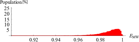
However, these results do not guarantee that the entanglement distributions themselves obtained by the Hamiltonians coincide with that of the typical entanglement. We show the calculations of the entanglement distributions for for , and the typical entanglement in Fig. 7. For each Hamiltonian, is set to the value that achieves the average amount of the typical entanglement. The entanglement distributions obtained by these Hamiltonians are clearly different from that of the typical entanglement for . In these cases, the entanglement distributions obtained by Hamiltonian dynamics is concentrated around the values higher than that of the distribution of the typical entanglement. Such properties of the entanglement distributions obtained by Hamiltonian dynamics may be useful for applications requiring to use a set of states with a higher concentration of entanglement in terms of Meyer-Wallach measure.
 |
| (a) |
 |
| (b) |
 |
| (c) |
Next, we analyze the shortest time required to achieve . For and , is . For , is the center of Gaussian of the distribution of the coupling constant . Thus the average amount of entanglement is achievable in a time scales independent of . On the other hand, for and , is inversely proportional to the strength of the neighboring -body interaction, , which is determined by the details of the Hamiltonian. If scales with , then . Because is necessary in order to achieve , the time required to achieve is also polynomial in . On the other hand, if scales with , the time required to achieve by the Hamiltonian dynamics is exponential in .
VI Summary
In this paper, we have studied the entanglement distributions obtained by one dimensional spin-1/2 Ising-type Hamiltonians composed of several types of many-body interactions. We have shown that, when the time-independent Hamiltonian is composed of up to neighboring -body interactions, a set of states randomly selected during the time evolution generated by the Hamiltonian can simulate the entanglement distribution of the typical entanglement of random states in terms of both the average and the standard deviation. Our results imply that neighboring -body Ising-type interactions are not sufficient for generating high entanglement, even though the order of many-body interactions scales with the number of spins and the interactions are not local interactions in the sense defined by [19]. We have also shown that the time required to achieve such a distribution is polynomial in the systems size if the strength of neighboring -body interactions scales with .
On the other hand, when the Hamiltonian is composed of only neighboring -body interactions, site-dependent coupling constants and neighboring -body interactions are required to simulate the average amount of entanglement of the typical entanglement. Although the standard deviation does not coincide to that of the distribution of the typical entanglement, the time required to achieve the distribution to simulate the average amount of entanglement alone is shown to be independent of the system size in this case.
Acknowledgements.
The authors thank P. S. Turner for helpful discussions and A. Tanaka for useful comments. This work was supported by Project for Developing Innovation Systems of the Ministry of Education, Culture, Sports, Science and Technology (MEXT), Japan. Y. N. acknowledges support from JSPS by KAKENHI (Grant No. 222812) and M. M. acknowledges support from JSPS by KAKENHI (Grant No. 23540463).Appendix A Derivation of the initial state
In this appendix, we show that the initial state gives the maximal average amount of entanglement , if the eigenstates of the Hamiltonian and the initial state are all separable.
In [23], we have introduced phase-random states, a set of pure states with fixed amplitudes and uniformly distributed phases in a fixed basis and derive a formula for the average amount of linear entropy of entanglement of phase random states for every possible bipartite partition. We have analyzed the entanglement evolution generated by a general Hamiltonian denoted by
where are eigenstates, from an initial state denoted by
| (21) |
where and . Under the assumption of phase ergodicity in the sense that the distribution of phases of are uniform in in the long-time limit, the infinite-time average of the amount of entanglement coincides to the average amount of entanglement of phase random states . From the formula for , it is straightforward to derive the following lemma in terms of the Mayer-Wallach measure of entanglement.
Lemma 1
If the system exhibits phase ergodicity, then
| (22) |
where
and for
We use this lemma for the Ising-type Hamiltonians and for separable initial states. We denote the eigenstates of the Ising-type Hamiltonian in the Pauli basis by using the binary representation defined by
| (23) |
Using this notation, the time evolution of the state generated by from a general initial state given by Eq. (21) is written by
| (24) |
where is the eigenenergy corresponding to .
Assuming phase ergodicity, the average amount of entanglement is obtained by using the lemma. Since the eigenstate is a separable state for all , , is given by
| (25) |
where
The right hand side of Eq. (25) can be written in terms of by
| (26) |
where and and the summations are taken over and . By using the normalization condition of , the first term of Eq. (26) is evaluated as
The equality holds if and only if for any .
On the other hand, a lower bound of the second terms of Eq. (26) is given by
since the arithmetic mean is always greater than or equal to the geometric mean. The equality holds if and only if does not depend on . By substituting these relations, the upper bound of the average is obtained by
where the equality holds if and only if the two conditions,
| (27) |
and
| (28) |
are simultaneously satisfied.
Since we consider a separable initial state , it must satisfy the condition for any , that is,
| (29) |
where and is the complex conjugate of . Under the conditions given by Eq. (27) and Eq. (29), we minimize so that we can obtain the maximum value of the average for separable initial states.
From Eq. (27) and Eq. (29), we obtain
With this condition, is easily maximized by Lagrange’s method of undetermined multipliers such as
where the equality holds if and only if and is constant for any , and . Therefore, we have proven that, for any separable initial states,
The equality holds if and only if for any , and for any , and , which are equivalent to and for any . Thus, the initial state gives the maximum amount of average of entanglement. By dropping the global phase , we obtain .
Appendix B Upper and lower bounds of the average entanglement for
From the initial state given by Eq. (5), the time evolution of the state by the Hamiltonian is formally written by
| (30) |
where is the binary representation of the eigenstates of (and also ) introduced by Eq. (23), and is the eigenenergy corresponding to given by
| (31) |
Since the Hamiltonian is translationally invariant, the Meyer-Wallach measure is given by . By calculating the reduced density matrix of given by Eq. (30), the Mayer-Wallach measure is obtained by
| (32) |
where . From Eq. (31), is given by
| (33) |
To calculate the bounds of , it is sufficient to evaluate the term . This term gives one for and zero for . By defining a quantity by
we obtain
From Eq. (33), we see that depends on for where , but it does not depend on for . By introducing a vector notation , in Eq. (32) is only determined by and . We define a quantity , which is the number of pairs satisfying . Then can be expressed in terms of by
where the factor appears due to the choice of and for . Recall that () is independent of () for . Thus, we obtain
We evaluate the upper and lower bounds of . For the lower bound, when , is trivially satisfied. Since the number of choices of is , we obtain . It is cumbersome to derive the upper bound of , but direct investigation of the expression of Eq. (33) provides a bound . Therefore, the upper and lower bounds of are
References
- [1] C. H. Bennett, P. Hayden, D. W. Leung, P. W. Shor and A. Winter, IEEE Trans. Inform. Theory, vol. 51, no. 1, pp 56-74 (2005).
- [2] B. M. Terhal, D. P. DiVincenzo and D. W. Leung, Phys. Rev. Lett. 86, 5807-5810 (2001).
- [3] D. P. DiVincenzo, D. W. Leung and B. M. Terhal, IEEE Trans. Inf Theory Vol. 48. No. 3, 580-599 (2002)
- [4] P. Hayden, D. Leung, P. W. Shor and A. Winter Commun. Math. Phys. 250(2):371-391(2004).
- [5] S. Goldstein, J. L. Lebowitz, R. Tumulka and N. Zanghi Phys. Rev. Lett. 96, 050403 (2006).
- [6] S. Popescu, A. J. Short and A. Winter, Nature Physics, 2:754-758 (2006).
- [7] N. Linden, S. Popescu, A. J. Short and A. Winter, Phys. Rev. E 79, 061103 (2009).
- [8] P. Hayden and J. Preskill, JHEP 0709:120 (2007).
- [9] P. Hayden, D. W. Leung and A. Winter, Comm. Math. Phys. Vol. 265, No. 1, pp. 95-117 (2006).
- [10] J. Emerson, Y. S. Weinstein, M. Saraceno and S. Lloyd and D. G. Cory, Science 302, 2098 (2003).
- [11] A. Ambainis and J. Emerson, IEEE Conference on Computational Complexity 2007, 129-140(2007).
- [12] R. Oliveira, O. C. O. Dahlsten and M. B. Plenio, Phys. Rev. Lett. 98, 130502 (2007).
- [13] O. C. O. Dahlsten, R. Oliveira and M. B. Plenio, J. Phys. A: Math. Theor. 40 8081-8108 (2007).
- [14] A. D. K. Plato, O. C. Dahlsten and M. B. Plenio, Phys. Rev. A 78, 042332 (2008).
- [15] A. W. Harrow and R. A. Low, Comm. Math. Phys. Vol. 291, No. 1, pp. 257-302 (2009).
- [16] A. J. Scott and C. M. Caves, J. Phys. A 36, 9553 (2003).
- [17] R. F. Abreu and R. O. Vallejos, Phys. Rev. A 73, 052327 (2006).
- [18] G. Benenti, La Rivista del Nuovo Cimento 32 (03), 105-146 (2009).
- [19] S. Bravyi, M. B. Hastings and F. Verstraete, Phys. Rev. Lett. 97, 050401 (2006).
- [20] H. Weimer, M. Muller, I. Lesanovsky, P. Zoller and H. P. Buchle, Nature Physics 6, 382 - 388 (2010).
- [21] D. A. Meyer and N. R. Wallach, J. Math. Phys. 43 4273 (2002).
- [22] G. K. Brennen, Quantum Information and Computation, vol. 3 (6), 619-626 (2003)
- [23] Y. Nakata, P. S. Turner and M. Murao, arXiv:1111.2747.