EFI 11-23
August 1, 2011
Model independent determination of the axial mass parameter in quasielastic neutrino-nucleon scattering
Bhubanjyoti Bhattacharya, Richard J. Hill and Gil Paz
Enrico Fermi Institute and Department of Physics
The University of Chicago, Chicago, Illinois, 60637, USA
Quasielastic neutrino-nucleon scattering is a basic signal process for neutrino oscillation studies. At accelerator energies, the corresponding cross section is subject to significant uncertainty due to the poorly constrained axial-vector form factor of the nucleon. A model-independent description of the axial-vector form factor is presented. Data from the MiniBooNE experiment for quasielastic neutrino scattering on 12C are analyzed under the assumption of a definite nuclear model. The value of the axial mass parameter, , is found to differ significantly from extractions based on traditional form factor models. Implications for future neutrino scattering and pion electroproduction measurements are discussed.
1 Introduction
High statistics neutrino experiments are probing the hadronic structure of nuclear targets at accelerator energies with ever greater precision. Extracting the underlying weak-interaction parameters, or new physics signals, requires similar precision in the theoretical description of the strong interactions.
A basic cross section describes the charged-current quasielastic scattering process on the neutron,
| (1) |
Recent evidence indicates a tension between measurements of this process in neutrino scattering at low [1, 2, 3, 4] and high [5] neutrino energies, and between results from neutrino scattering and results inferred from pion electroproduction [6]. In particular, with a commonly used dipole ansatz for the axial-vector form factor of the nucleon,
| (2) |
different experiments have reported values for the so-called axial mass parameter . World averages reported by Bernard et al. [6] find comparable values obtained from neutrino scattering results prior to 1990, , and from pion electroproduction, .11 1 The difference is a correction to the conventional representation of the pion electroproduction amplitude, as predicted by heavy baryon chiral perturbation theory [6]. The NOMAD collaboration reports [5] . In contrast, MiniBooNE reports [3] GeV, and other recent results from the K2K SciFi [1], K2K SciBar [7] and MINOS [8] collaborations similarly find central values higher than the above-mentioned world average. Quasielastic neutrino-nucleon scattering (1) is a basic signal process in neutrino oscillation studies. It is essential to obtain consistency between experiments utilizing different beam energies, and different nuclear targets.
While a number of effects could be causing this tension, we here investigate perhaps the simplest possibility: that the parameterizations of the axial-vector form factor in common use are overly constrained. Such a possibility seems natural, considering that the dipole ansatz has been found to conflict with electron scattering data for the vector form factors. We do not offer new insight on whether other effects, such as nuclear modeling, could also be biasing measurements. However, we point out that by gaining firm control over the nucleon-level amplitude, such nuclear physics effects can be robustly isolated.
The axial mass parameter as introduced in (2) is not well-defined, since the true form factor of the proton does not have a pure dipole behavior. Sufficiently precise measurements forced to fit this functional form will necessarily find different values for resulting from sensitivity to different ranges of . Let us define the axial mass parameter in terms of the form factor slope at : . This definition is model-independent, and allows us to sensibly address tensions between different measurements. To avoid confusion, whenever (2) is used we refer to the extracted parameter as . We will show that the slope at is essentially the only relevant shape parameter for current data at , and introduce the formalism to systematically account for the impact of other poorly constrained shape parameters on the determination of . A related study of the vector form factors of the nucleon was presented in [9].
The paper is structured as follows. In Section 2 we discuss the application of analyticity and dispersion relations to the axial-vector form factor of the nucleon. Section 3 presents results for the extraction of the axial-vector form factor slope from MiniBooNE data. We illustrate constraints imposed by our analysis on nuclear models, by determining the binding energy parameter in the Relativistic Fermi Gas (RFG) model of Smith and Moniz [16]. Section 4 gives an illustrative analysis of constraints on the axial mass parameter from pion electroproduction data. Section 5 discusses the implications of our results. For completeness, Appendix A collects formulas for the RFG nuclear model.
2 Analyticity constraints
This section provides form factor definitions and details of the model-independent parameterization based on analyticity.
2.1 Form factor definitions
The nucleon matrix element of the Standard Model weak charged current is
| (3) |
where , and we have enforced time-reversal invariance and neglected isospin-violating effects as discussed in Appendix A. The vector form factors and can be related via isospin symmetry to the electromagnetic form factors measured in electron-nucleon scattering. At low energy, the form factors are normalized as , . For definiteness we take a common nucleon mass, . Parameter values used in the numerical analysis are listed in Table 2. In applications to quasielastic electron- or muon-neutrino scattering, the impact of is suppressed by powers of the small lepton-nucleon mass ratio. For our purposes, the pion pole approximation is sufficient,22 2 Here and throughout, denotes the pion mass.
| (4) |
The axial-vector form factor is normalized at by neutron beta decay (see Table 2). Our main focus is on determining the dependence of in the physical region of quasielastic neutrino scattering, . As discussed in the Introduction, an expansion at defines an “axial mass parameter” , via
| (5) |
Equivalently, we may define an “axial radius” , via
| (6) |
The factors appearing in (5) and (6) are purely conventional, motivated by the dipole ansatz (2), and by the analogous charge-radius definition for the vector form factors. Asymptotically, perturbative QCD predicts [10, 11] a scaling, up to logarithms, for the axial-vector form factor. However, the region is far from asymptotic, and the functional dependence of remains poorly constrained at accessible neutrino energies.
2.2 Analyticity

We proceed along lines similar to the vector form factor analysis in [9]. Recall the dispersion relation for the form factor,
| (7) |
where and the integral starts at the three-pion cut, . We can make use of this model-independent knowledge by noticing that the separation between the singular region, , and the kinematically allowed physical region, , implies the existence of a small expansion parameter, . As illustrated in Fig. 1, by a standard transformation, we map the domain of analyticity onto the unit circle in such a way that the physical region is mapped onto an interval:
| (8) |
where is a free parameter representing the point mapping onto . Analyticity implies that the form factor can be expressed as a power series in the new variable,
| (9) |
The coefficients are bounded in size, guaranteeing convergence of the series. Knowledge of over the cut translates into information about the coefficients in the expansion [9]. In particular we have
| (10) |
where
| (11) |
2.3 Coefficient bounds
For a given kinematic range , we can choose the free parameter in (8) to minimize the resulting maximum size of . It is straightforward to see that the “optimal” value of is , and for this value of , . For example, if the kinematic range is , then our expansion parameter is constrained to be . Terms beyond linear order in the expansion are suppressed by , etc., and are not tightly constrained by current experimental data. This is the sense in which the slope of the form factor (conventionally taken at ) is essentially the only relevant shape parameter. The effects of the higher order terms must of course be accounted for in assessing the uncertainty on extracted observables. We now turn to this question.
| 1.5-1.7 | 1.9-2.3 | |
| 1.0-1.4 | 1.4-1.8 |
The expansion coefficients appearing in (9) can be used to define norms,
| (12) |
In particular, provides a bound on the maximum coefficient size. The finiteness of the integral appearing in the relation
| (13) |
together with , establishes that a finite upper bound exists for the coefficients. As a first approach to estimating the actual bound , consider an “axial-vector dominance” ansatz, , where and are the mass and width of the lowest lying axial-vector, iso-vector meson [12]. More precisely, let us define the form factor via its dispersion relation with [13]
| (14) |
where is a normalization constant determined below. Using the dispersion relation (7) with (14) we find,
| (15) |
where , and is determined by the value of . Table 1 displays the values for and computed in this ansatz. For the latter quantity one can show that
| (16) |
While this model is not a rigorous description of the true spectral function in (7), it indicates an order unity bound on the coefficients appearing in (9). Additional support for an order unity bound is provided by a related detailed study of nucleon vector form factors [9], and by form factor studies in a wide range of meson transitions [14, 15].
In the following numerical analysis, we follow [9], and investigate fits with various bounds on coefficients, e.g. and .
3 Extraction of the axial mass parameter
The MiniBooNE collaboration has presented binned results representing the double differential cross section, , for the quasielastic scattering process (1) on a neutron bound inside 12C. We apply our description of to extract (equivalently, ) from the neutrino scattering data, under the assumption of a definite nuclear model, the Relativistic Fermi Gas model [16] as described in Appendix A.
| Parameter | Value | Reference |
|---|---|---|
| 0.9742 | [12] | |
| 2.793 | [12] | |
| [12] | ||
| 0.1057 GeV | [12] | |
| GeV-2 | [12] | |
| 0.9389 GeV | [12] | |
| [12] | ||
| 0.025 GeV | [17] | |
| 0.220 GeV | [3] |
Our theory prediction is obtained using (54), integrating over the energy-dependent flux from Table V of [3]; this result is divided by to obtain the per-neutron event rate, and divided by the total flux to obtain the flux-averaged cross section. Corresponding experimental values for the double differential cross section are taken from Table VI of [3]. We form an error matrix,
| (17) |
where denotes a partial cross section, denotes the shape uncertainty from Table VII of [3], and is the normalization error from [3]. We form the chi-squared function
| (18) |
and minimize to find best fit values for . Error intervals are defined by . The nucleon form factors and the nuclear model employ parameter values listed in Table 2. Following the analysis of [3], the vector form factors and are given by the BBA2003 parameterization [18]. We use a default value GeV, as extracted from electron scattering data on nuclei in [17]. This value is different from the central value adopted in the MiniBooNE analysis [3], where GeV. We show below that such a high value of is not favored by the MiniBooNE data, but investigate fit results for different values of .
The slope at , and hence from (5) is most sensitive to low- data. We analyze this sensitivity by considering the effect of a cut on . The value of for a given value of the observed muon energy and angle can be reconstructed assuming quasielastic scattering on a free neutron, but is not determined unambiguously once nuclear effects are included. As a proxy for , we define an approximate “reconstructed” ,
| (19) |
where approximates the neutrino energy in the nucleon rest frame,
| (20) |
We note that coincides with used by K2K in the limit [1], and with used by MiniBooNE in the limit and equal proton and neutron masses [3]. For simplicity we have chosen to make the cut independent of the binding energy used in the nuclear model. We emphasize that this choice is used simply to define the subset of data to be analyzed, and does introduce theoretical uncertainty in the numerical results.
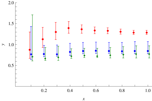
Our results are displayed in Fig. 2, where we compare extractions of in the dipole ansatz (2) with extractions of employing the expansion (9). We present results for data with , where is defined in (19) and . We study two different coefficient bounds, and . For definiteness we have truncated the sum in (9) at , but have checked that the results do not change significantly if higher orders are included. As Fig. 2 illustrates, the expansion results lie systematically below results assuming the dipole ansatz. In contrast to results from the one-parameter dipole ansatz, high- data have relatively small impact on the model-independent determination of . Taking for definiteness , we find
| (21) |
where the first error is experimental, using the fit with , and the second error represents residual form factor shape uncertainty, taken as the maximum change of the interval when the bound is increased to . As a comparison, a fit assuming the dipole form factor, and the same yields GeV.33 3 A dipole fit including the entire dataset without a cut on yields .
It is not our purpose in this paper to investigate in detail the additional uncertainty that should be assigned to (21) due to nuclear effects. We note that a fit of the MiniBooNE data to the RFG model with free parameter yields the value, without an assumption on the value of , (for , )
| (22) |
where the result is insensitive to the choice of bound, or .44 4 Using a dipole ansatz for without fixing yields . While the data do not appear to favor significantly higher values of , we note that for [3], the result (21) becomes , compared to .
We have performed fits at different values of the parameter , finding no significant deviation in the results. The results do not depend strongly on the precise value of the bound (e.g. versus ). Similar to [9], we conclude that the estimation of shape uncertainty in (21) should be conservative. The fit (21) yields coefficients55 5 For this purpose we take in (9) and enforce for . , , . These values are in accordance with our assumption of order-unity coefficient bounds. As discussed in the Introduction, current experiments do not significantly constrain shape parameters beyond the linear term, .
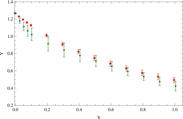
Figure 3 compares the form factor extraction resulting from the expansion fit to the extraction from the dipole fit. Here we take , and for the fit. The dipole fit assumes .
4 Comparison to charged pion electroproduction

The axial-vector component of the weak current defining in (3) can also be probed in pion electroproduction measurements. The electric dipole amplitude for threshold charged-pion electroproduction obeys a low-energy theorem in the chiral limit relating this amplitude to the axial-vector form factor of the nucleon [19]. After applying chiral corrections, such measurements can thus in principle be used to determine . Data for this process have been interpreted in the context of the dipole ansatz (2). We found that the dipole assumption can strongly bias extractions of in neutrino scattering measurements. In order to gauge whether the same statement is true for the electroproduction data, let us apply the expansion to extract from the inferred values for an illustrative dataset, taken from Refs. [20, 21, 22, 23, 24]. We have selected datasets that appear in the compilation [6] (cf. Figure 1 of that reference), and that also explicitly list inferred values of (see also [25, 26, 27, 28, 29]). Figure 4 displays extractions of in both the expansion and the dipole ansatz (2) for each of the five datasets.66 6 For definiteness, where necessary we have chosen one amongst different models for applied hard-pion corrections: the BNR prescription [30] in [22, 23, 24], and the BNR prescription with first form factor assumption in [20] (“” in Table 2 of [20] ). We have combined the low- and high- data from [22] and [23] to obtain the Daresbury(1975/1976) data point in Fig. 4. For the larger bound , the slope of is not constrained to be positive by each individual dataset, and we display only the result for . Applying the expansion to the entire (17 point) dataset, we find
| (23) |
where the errors are experimental, and from residual shape uncertainty, as in (21). In contrast, a fit of the same data to the dipole ansatz yields . These averages are also displayed in the figure. We emphasize that our chosen dataset is not exhaustive We have not attempted to address questions such as correlations between different datasets, or uncertainties from model-dependent hard-pion corrections. We leave a more detailed treatment to future work.
5 Summary
We have presented a model independent description of the axial-vector form factor of the nucleon. This form factor plays a crucial role in neutrino quasielastic scattering at accelerator energies, which is a basic signal process for neutrino oscillation studies, and is an important ingredient in normalizing the neutrino flux at detector locations. Recent tensions between measurements in neutrino scattering at different energies, and between neutrino scattering and pion electroproduction measurements indicate a problem in our understanding of this elementary process.
Several studies have tried to address these discrepancies. Modified nuclear models [31, 32, 33] have been used to find an axial mass close to the MiniBooNE result. Other nuclear models include effects of multi-nucleon emission [34, 35, 36, 37, 38, 39], and have been reported to obtain better agreement with the differential MiniBooNE data from [3]. One of these studies [39] reports a dipole axial mass extracted from MiniBooNE data in agreement with world averages from [6, 5]. Another group [40], modifies the magnetic form factor for nucleons bound in carbon but does not change the form factors or . The assumption of the dipole ansatz (2) is a crucial element in many of these studies.77 7 A parameterization that modifies the dipole behavior at large is presented in [41]. Our analysis shows that this ansatz introduces a strong bias in measurements, which must be addressed in order to disentangle nucleon-level interactions from nuclear effects.
Under the assumption of a definite nuclear model (the RFG model, summarized in Appendix A, with parameter values as in Table 2), we extract as defined model-independently in (5) from the differential MiniBooNE data [3]. The result is displayed in (21), . This result may be contrasted with a fit to an illustrative dataset for pion electroproduction displayed in (23), . These values may be compared to fits using the dipole ansatz (2): (neutrino scattering) and (electroproduction). A discrepancy is apparent in the dipole ansatz (2), but can be ascribed to the unjustified and restrictive assumption on the form factor shape. After gaining firm control over the nucleon-level amplitude, nuclear effects can be robustly isolated. For example, in the context of the RFG model, we extract the result (22) for the binding energy parameter .
The axial mass parameter, or equivalently, the axial radius (6), is a fundamental parameter of nucleon structure. The results (21),(23) can be expressed as
| (24) |
More precise measurements in both neutrino scattering and pion electroproduction are necessary to substantially reduce the errors on , or equivalently . This would be necessary to provide a model-independent confirmation of the convergence of chiral perturbation theory corrections based on comparison of electroproduction and neutrino scattering data.
A related study of the nucleon vector form factors was presented in [9]. As described there, different expansion “schemes” are possible. For example, we may replace (9) with , where is analytic below . A choice such as with could be used to enforce a falloff for asymptotic , while retaining the known analytic structure of the form factor. Such modifications do not significantly impact the extraction of , and we have focused on the simplest choice ( and ).
Our study indicates that the error on the axial mass parameter extracted using the dipole ansatz is underestimated. While the errors from a model-independent analysis may be larger, it is essential to study model-independent numbers in order to draw firm conclusions. The simulation of more complicated neutrino scattering processes (e.g. pion and photon production), is indirectly affected by enforcing agreement with the quasielastic data. It is important for current and future neutrino experiments [42, 43, 44, 45, 5, 46, 3, 47, 48, 49] to converge on consistent values for fundamental neutrino cross sections.
The analysis presented here can be applied to other neutrino scattering datasets, involving different nuclear targets, and including neutral current scattering and antineutrino scattering. It is interesting to extend the analysis of electroproduction data; more precise low-energy electroproduction measurements have potential to impact the interpretation of future neutrino measurements. It is also of interest to incorporate model-independent constraints into more sophisticated nuclear models.
Acknowledgements
We thank T. Katori for useful discussions with respect to the MiniBooNE analysis, and V. Bernard, L. Elouadrhiri and U.-G. Meissner for supplying data corresponding to Figure 2 of [6]. Work supported by NSF Grant 0855039 and DOE grant DE-FG02-90ER40560.
Appendix A Appendix: RFG model for quasielastic neutrino scattering
A number of notations and conventions for the form factors and RFG nuclear model [16] exist in the literature. For completeness we collect here the relevant formulas used in our analysis.
A.1 Nucleon matrix element of the weak current
The relevant part of the weak-interaction Lagrangian is
| (25) |
The cross section for on a free neutron is
| (26) |
where the spin-averaged, squared amplitude is
| (27) |
The leptonic tensor neglecting the neutrino mass is ()
| (28) |
The hadronic matrix element appearing in (27) is parameterized by
| (29) |
where and we have defined the vertex function
| (30) |
We may write the cross section of (26) as
| (31) |
where the nucleon structure function is
| (32) |
The hadronic tensor is
| (33) |
where as usual, . We may similarly analyze antineutrino scattering, , using (31), taking , and making the replacements , in .
Imposing time-reversal invariance shows that are real. We will assume isospin symmetry in the following, in which case and vanish, , and . The hadronic tensor has the time-reversal invariant decomposition
| (34) |
The ’s are expressed in terms of the form factors as
| (35) |
Expressions for complex and nonzero , can be found, for example, in [50].
A.2 Model for the nuclear matrix element
We employ a standard treatment of nuclear effects, the “Relativistic Fermi Gas” (RFG) model as presented by Smith and Moniz in [16], based on the model presented in [51].
We assume that there are nucleons inside the nucleus, with neutrons and protons. The incoming neutrino interacts with a neutron with 3-momentum , determined by some distribution . The final state proton phase space is limited by a factor of enforcing Fermi statistics. Symbolically,
| (36) |
and more explicitly
| (37) |
To arrive at the final model, two modifications are made. First, we make the replacement in the prefactor of (37). This replacement ignores a correction from the nonzero velocity of the initial state nucleon. It corresponds to the model of [16], adopted by [3]; for definiteness we have followed this convention. Second, we incorporate a “binding energy”, , by expressing as a function of Lorentz 4-vectors , as in (34) and then making in (37) the replacements
| (38) |
with . Again, there is some arbitrariness to the insertion of into the formalism; for definiteness we have followed the conventions of [16]. The cross section is then
| (39) |
where is the 4-momentum of the target nucleus with mass . We work in the target rest frame where . The model nuclear structure function is defined as
| (40) |
with
| (41) |
The distribution of neutrons and protons is
| (42) |
where is a parameter of the model. The normalization is fixed by requiring neutrons below the Fermi surface (accounting for 2 fermionic spin states),
| (43) |
We can expand in a similar way to in (34):
| (44) |
The functions are related to integrals over . The relations can be expressed in terms of the following integrals [16]:
| (45) | |||||
where and the axis is parallel to . A straightforward but tedious comparison shows that
| (46) |
where we are using . Recall that the are functions of . For the integrals let us define , and observe that
| (47) |
The integrals can be expressed in terms of
| (48) |
for . In particular,
| (49) |
Up to an overall constant these are the ’s of [16]. Introducing , , we can express the ’s as
| (50) |
The range of integration is restricted by the conditions,
| (51) |
The latter condition can be expressed as
| (52) |
Define
| (53) |
Then if , there is no contribution for the given kinematics.
In the rest frame of the nucleus, let and be the energy and 3-momentum of the charged lepton, and let be the angle between the -momenta of the leptons. From (39), the final expression for the differential cross section of neutrino-nucleus scattering is
| (54) |
where are given in (46), and where the upper (lower) sign is for neutrino (anti-neutrino) scattering.
References
- [1] R. Gran et al. [K2K Collaboration], Phys. Rev. D 74, 052002 (2006) [arXiv:hep-ex/0603034].
- [2] A. A. Aguilar-Arevalo et al. [MiniBooNE Collaboration], Phys. Rev. Lett. 100, 032301 (2008) [arXiv:0706.0926 [hep-ex]].
- [3] A. A. Aguilar-Arevalo et al. [ MiniBooNE Collaboration ], Phys. Rev. D81, 092005 (2010). [arXiv:1002.2680 [hep-ex]].
- [4] A. A. Aguilar-Arevalo et al. [MiniBooNE Collaboration], Phys. Rev. D 82, 092005 (2010) [arXiv:1007.4730 [hep-ex]].
- [5] V. Lyubushkin et al. [NOMAD Collaboration], Eur. Phys. J. C 63, 355 (2009) [arXiv:0812.4543 [hep-ex]].
- [6] V. Bernard, L. Elouadrhiri and U. G. Meissner, J. Phys. G 28, R1 (2002) [arXiv:hep-ph/0107088].
- [7] X. Espinal and F. Sanchez, AIP Conf. Proc. 967, 117 (2007).
- [8] M. Dorman [MINOS Collaboration], AIP Conf. Proc. 1189, 133 (2009).
- [9] R. J. Hill and G. Paz, Phys. Rev. D 82, 113005 (2010) [arXiv:1008.4619 [hep-ph]].
- [10] G. P. Lepage and S. J. Brodsky, Phys. Rev. D 22, 2157 (1980).
- [11] C. E. Carlson and J. L. Poor, Phys. Rev. D 34, 1478 (1986).
- [12] K. Nakamura et al. [Particle Data Group], J. Phys. G 37, 075021 (2010).
- [13] J. Schwinger, Annals Phys. 9, 169-193 (1960).
- [14] For a review and further references see: R. J. Hill, In the Proceedings of 4th Flavor Physics and CP Violation Conference (FPCP 2006), Vancouver, British Columbia, Canada, 9-12 Apr 2006, pp 027, [arXiv:hep-ph/0606023].
- [15] C. Bourrely, B. Machet and E. de Rafael, Nucl. Phys. B 189, 157 (1981). C. G. Boyd, B. Grinstein and R. F. Lebed, Phys. Rev. Lett. 74, 4603 (1995) [arXiv:hep-ph/9412324]. L. Lellouch, Nucl. Phys. B 479, 353 (1996) [arXiv:hep-ph/9509358]. M. C. Arnesen, B. Grinstein, I. Z. Rothstein and I. W. Stewart, Phys. Rev. Lett. 95, 071802 (2005) [arXiv:hep-ph/0504209]. C. G. Boyd, B. Grinstein and R. F. Lebed, Nucl. Phys. B 461, 493 (1996) [arXiv:hep-ph/9508211]. I. Caprini, L. Lellouch and M. Neubert, Nucl. Phys. B 530, 153 (1998) [arXiv:hep-ph/9712417]. T. Becher and R. J. Hill, Phys. Lett. B 633, 61 (2006) [arXiv:hep-ph/0509090]. R. J. Hill, Phys. Rev. D 74, 096006 (2006) [arXiv:hep-ph/0607108]. A. Bharucha, T. Feldmann and M. Wick, arXiv:1004.3249 [hep-ph]. C. Bourrely, I. Caprini and L. Lellouch, Phys. Rev. D 79, 013008 (2009) [arXiv:0807.2722 [hep-ph]].
- [16] R. A. Smith and E. J. Moniz, Nucl. Phys. B 43, 605 (1972) [Erratum-ibid. B 101, 547 (1975)].
- [17] E. J. Moniz, I. Sick, R. R. Whitney, J. R. Ficenec, R. D. Kephart and W. P. Trower, Phys. Rev. Lett. 26, 445 (1971).
- [18] H. S. Budd, A. Bodek and J. Arrington, arXiv:hep-ex/0308005.
- [19] Y. Nambu and D. Lurie, Phys. Rev. 125, 1429 (1962). Y. Nambu and E. Shrauner, Phys. Rev. 128, 862 (1962).
- [20] E. Amaldi et al., Phys. Lett. B 41, 216 (1972).
- [21] P. Brauel et al., Phys. Lett. B 45, 389 (1973).
- [22] A. Del Guerra et al., Nucl. Phys. B 99, 253 (1975).
- [23] A. Del Guerra et al., Nucl. Phys. B 107, 65 (1976).
- [24] A. S. Esaulov, A. M. Pilipenko and Yu. I. Titov, Nucl. Phys. B 136, 511 (1978).
- [25] E. Amaldi et al., Nuovo Cim. A 65, 377 (1970).
- [26] E. D. Bloom et al., Phys. Rev. Lett. 30, 1186 (1973).
- [27] P. Joos et al., Phys. Lett. B 62, 230 (1976).
- [28] S. Choi et al., Phys. Rev. Lett. 71, 3927 (1993).
- [29] A. Liesenfeld et al. [A1 Collaboration], Phys. Lett. B 468, 20 (1999) [arXiv:nucl-ex/9911003].
- [30] G. Benfatto, F. Nicolo and G. C. Rossi, Nucl. Phys. B 50, 205 (1972). G. Benfatto, F. Nicolo and G. C. Rossi, Nuovo Cim. A 14, 425 (1973).
- [31] A. V. Butkevich, Phys. Rev. C82, 055501 (2010). [arXiv:1006.1595 [nucl-th]].
- [32] O. Benhar, P. Coletti, D. Meloni, Phys. Rev. Lett. 105, 132301 (2010). [arXiv:1006.4783 [nucl-th]].
- [33] C. Juszczak, J. T. Sobczyk, J. Zmuda, Phys. Rev. C82, 045502 (2010). [arXiv:1007.2195 [nucl-th]].
- [34] M. Martini, M. Ericson, G. Chanfray, J. Marteau, Phys. Rev. C80, 065501 (2009). [arXiv:0910.2622 [nucl-th]].
- [35] M. Martini, M. Ericson, G. Chanfray, J. Marteau, Phys. Rev. C81, 045502 (2010). [arXiv:1002.4538 [hep-ph]].
- [36] J. E. Amaro, M. B. Barbaro, J. A. Caballero, T. W. Donnelly, C. F. Williamson, Phys. Lett. B696, 151-155 (2011). [arXiv:1010.1708 [nucl-th]].
- [37] J. E. Amaro, M. B. Barbaro, J. A. Caballero, T. W. Donnelly, J. M. Udias, Phys. Rev. D84, 033004 (2011). [arXiv:1104.5446 [nucl-th]].
- [38] J. Nieves, I. Ruiz Simo, M. J. Vicente Vacas, Phys. Rev. C83, 045501 (2011). [arXiv:1102.2777 [hep-ph]]
- [39] J. Nieves, I. R. Simo, M. J. V. Vacas, [arXiv:1106.5374 [hep-ph]].
- [40] A. Bodek and H. Budd, Eur. Phys. J. C 71, 1726 (2011) [arXiv:1106.0340 [hep-ph]].
- [41] A. Bodek, S. Avvakumov, R. Bradford and H. S. Budd, Eur. Phys. J. C 53, 349 (2008) [arXiv:0708.1946 [hep-ex]].
- [42] D. Drakoulakos et al. [Minerva Collaboration], arXiv:hep-ex/0405002. D. A. Harris et al. [MINERvA Collaboration], arXiv:hep-ex/0410005.
- [43] D. S. Ayres et al. [NOvA Collaboration], arXiv:hep-ex/0503053.
- [44] A. A. Aguilar-Arevalo et al. [SciBooNE Collaboration], arXiv:hep-ex/0601022.
- [45] H. Chen et al. [MicroBooNE Collaboration], Fermilab proposal 0974.
- [46] M. C. Sanchez [LBNE DUSEL Collaboration], AIP Conf. Proc. 1222, 479 (2010). V. Barger et al., arXiv:0705.4396 [hep-ph].
- [47] S. D. Holmes [Project X Collaboration], In the Proceedings of 1st International Particle Accelerator Conference: IPAC’10, Kyoto, Japan, 23-28 May 2010, pp TUYRA01. See also: https://www.ids-nf.org/wiki/FrontPage/Documentation/IDR .
- [48] K. Abe et al. [T2K Collaboration], arXiv:1106.1238 [Unknown]. K. Abe et al. [ T2K Collaboration ], Phys. Rev. Lett. 107, 041801 (2011). [arXiv:1106.2822 [hep-ex]].
- [49] S. Choubey et al., “International Design Study for the Neutrino Factory, Interim Design Report,” IDS-NF-20, March 2011.
- [50] K. S. Kuzmin, V. V. Lyubushkin and V. A. Naumov, Eur. Phys. J. C 54, 517 (2008) [arXiv:0712.4384 [hep-ph]].
- [51] E. J. Moniz, Phys. Rev. 184, 1154 (1969).