The Magnetic Field in Taurus Probed by Infrared PolarizationNote: Accepted in Astrophysical Journal
Abstract
We present maps of the plane-of-sky magnetic field within two regions of the Taurus molecular cloud: one in the dense core L1495/B213 filament, the other in a diffuse region to the west. The field is measured from the polarization of background starlight seen through the cloud. In total, we measured 287 high-quality near-infrared polarization vectors in these regions. In L1495/B213, the percent polarization increases with column density up to mag, the limits of our data. The Radiative Torques model for grain alignment can explain this behavior, but models that invoke turbulence are inconsistent with the data. We also combine our data with published optical and near-infrared polarization measurements in Taurus. Using this large sample, we estimate the strength of the plane-of-sky component of the magnetic field in nine subregions. This estimation is done with two different techniques that use the observed dispersion in polarization angles. Our values range from G and tend to be higher in denser regions. In all subregions, the critical index of the mass-to-magnetic flux ratio is sub-unity, implying that Taurus is magnetically supported on large scales ( pc). Within the region observed, the B213 filament makes a sharp turn to the north and the direction of the magnetic field also takes a sharp turn, switching from being perpendicular to the filament to becoming parallel. This behavior can be understood if we are observing the rim of a bubble. We argue that it has resulted from a supernova remnant associated with a recently discovered nearby gamma-ray pulsar.
Subject headings
dust,extinction—ISM: bubbles—ISM: clouds— ISM: individual (Taurus)—ISM: magnetic fields—PolarizationI. Introduction
It has been known for decades that observed starlight is polarized [16, 21]. This polarization is generally understood to be caused by non-spherical dust grains between Earth and the star that preferentially align with their long axes perpendicular to the local magnetic field direction. At optical to near-infrared wavelengths, the grains will preferentially absorb starlight that is linearly polarized parallel to their long axes. Thus, it is possible to probe the interstellar magnetic field by observing the polarized light because at optical and near-infrared wavelengths, the measured polarization angle will be parallel to the magnetic field direction.
The importance of magnetic fields to star formation is a hotly debated topic. Many to most molecular clouds are gravitationally bound, yet the observed star formation efficiency of clouds is only a few percent [37]. Magnetic fields are one mechanism that can provide cloud support against gravitational collapse [36]. An alternative theory is that magnetic fields are too weak to resist gravity and it is interstellar turbulence that regulates star formation [32].
The Taurus molecular cloud is an excellent target for exploring the importance of magnetic fields in molecular clouds. As one of the closest low-mass star-forming clouds at a distance of 140pc [11, 24, 51, 28, 29, 46], Taurus has been a frequent target for studies [25, see the extensive review by]. Furthermore, recent work has revealed a coupling between the gas and the magnetic field in Taurus. Goldsmith et al. [12] found striations in their 12CO data that matched the angle of the optical polarization vectors measured by Moneti et al. [35]. Goldsmith et al. offered two possible mechanisms to explain the striations and their observed alignment with the magnetic field. Large-scale flows are seen in the 12CO and 13CO channel maps; given the coupled magnetic field and gas, shear in these flows could explain the striations. Alternatively, a magnetosonic wave traveling perpendicular to the field could compress or rarefy the gas into the perceived striations. The filamentary region B213 in Taurus also has an apparent connection between the gas and the magnetic field. The optical and near-infrared polarization vectors are oriented perpendicular to the long axis of the filament [18, 14] implying that gravitational collapse has occurred along the field lines but not across them.
Several studies have measured the large-scale magnetic field in Taurus at optical wavelengths [35, 18, 13, 49], but only a handful of polarization vectors exist in the near-infrared [35, 45, 14]. Therefore, the magnetic field properties are poorly known in the high column density regions where stars form. Near-infrared observations are needed to penetrate these regions. To address this deficiency, in this paper we present 287 near-infrared polarization measurements towards two regions of Taurus. One region is towards B213 and L1495 and has not been mapped before in polarization. Since L1495 is the highest column density area of Taurus with the highest density of embedded young stellar objects, measuring the magnetic field in this region is important for studying the connection between magnetic fields and star formation. We also observed a diffuse region near where Goldsmith et al. [12] found striations in the 12CO that matched the angles of the optical polarization vectors.
In § II we discuss the observations, data reduction, and selection criteria to create the high-quality source catalogs. We also list references to previously published optical to near-infrared polarization studies in Taurus that will augment our new data set. We use these combined data sets to address several key magnetic field related questions and issues in § III. We discuss grain alignment efficiency (§ III.1), magnetic field strength (§ III.2), cloud stability (§ III.3), turbulence estimates in L1495 (§ III.4), and finally the magnetic field morphology in L1495 (§ III.5). We summarize our findings in § IV.
II. Observations
We used the Mimir instrument [7] to observe -band (m) polarization of background starlight seen through the Taurus molecular cloud. Mimir is installed on the 1.8m Perkins telescope located near Flagstaff, AZ and operated by Lowell Observatory. The observations spanned the nights of 2009 Jan. 12-16 UT. We observed two regions within Taurus: one in a low-density portion of the cloud (hereafter ‘Diffuse’) and the other toward a high-density region, B213/L1495 (hereafter ‘Filament’). The Diffuse region is rectangular covering roughly in Right Ascension and in Declination. The Filament region is not quite rectangular, but spans approximately to in Right Ascension and in Declination. Coordinates are J2000.
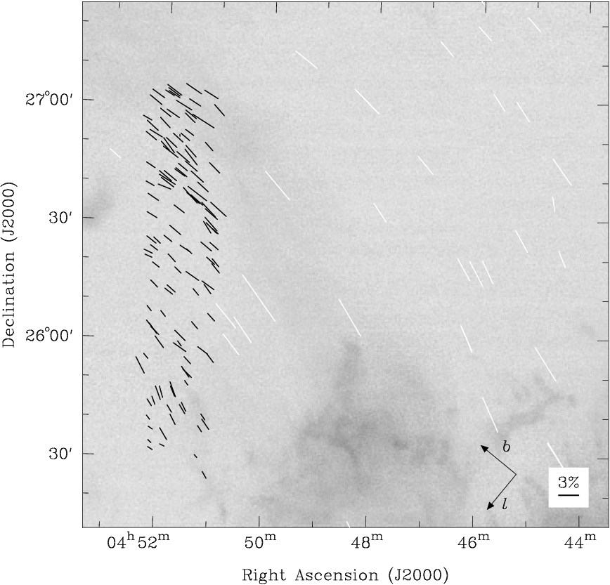
Each region consisted of an overlapping mosaic of Mimir fields-of-view. For each FOV, we observed in a six-position hex dither pattern where each dither position was offset by about from the center. At each dither position we obtained images at 16 angles of the half-wave plate (HWP), each separated by . The integration time per HWP angle was either 2.5s (short) or 10s (long). The 16 HWP positions are equivalent to observing four angles separated by four times each because the Stokes parameters vary as and because polarization “vectors” only have angle and not direction. Therefore, the effective integration time per pixel on the sky where all dithers overlap was s = 60s (short) and s = 240s (long). These times are for each of the four independent HWP angles. The short integrations provide polarization measurements for most sources that were saturated in the long integrations. The Diffuse region has low extinction, therefore we observed it only with short integrations. For the Filament region, we observed all but five fields with both short and long integrations. The two regions observed are indicated in Figure 1 as hashed (short) and cross-hatched (short and long). All previously published optical to near-infrared wavelength polarization measurements are shown as white and black vectors. See § II.2 for details on these catalogs.

We reduced the data using custom IDL programs (Clemens et al. in prep)11 1 The latest released software can be found at: http://people.bu.edu/clemens/mimir/software.html . Each field, both long and short integrations, was processed separately to create stellar polarization lists. We then separately combined the short and long integrations from the different fields into a single catalog. For stars that position matched within a star in adjacent field(s), we computed the weighted average of their Stokes parameters. Next we combined our short and long integrations in the Filament again using a matching radius. For stars that matched we always used the polarizations obtained from the long integrations, assuming they were more accurate. Stars saturated in the long integrations, however, did not have measured polarizations. Therefore, when combining the short and long integrations, these stars have polarizations derived from the short integrations.
II.1. High-Quality Vectors
We applied two selection criteria to the catalogs to produce the high-quality polarizations used in this paper. First, we selected only those data with percentage polarization divided by its uncertainty . Most of the sources removed by this criterion are faint and would also be removed by the second criterion. The low sources have median and median . Secondly, we required sources to be brighter than 12th mag. in the band for the short integrations and brighter than 13th mag. ( band) for the long integrations. The second criterion eliminated the few fainter sources not caught by the first criterion. The measured polarizations for fainter sources are unreliable because they are dominated by errors not accounted for by the first criterion (D. Clemens, private comm.). These magnitudes are the 2MASS magnitudes for each source. Five sources in the Diffuse region did not have 2MASS counterparts and all five were excluded from the final catalogs. Nine of the stars in the Filament region did not have 2MASS counterparts and they were also excluded.
The measured polarization from embedded protostars is not a useful probe of the magnetic field in molecular clouds. The radiation from the protostars may drive dust grain alignment, thus possibly altering the measured polarization. Furthermore, reflected light from the disk and envelope is highly polarized and non-uniform. To avoid this potential bias, we compared our polarization positions with those of the known protostellar members of Taurus from Luhman et al. [31]. None of our stars in the Diffuse region position matched within a known Taurus member. These 125 sources are listed in Table 1. In the Filament, 11 of the 173 polarization measurements matched within the positions of known Taurus members. After excluding these, 162 high-quality polarizations remained and these are listed in Table 2. Because protostars may have some nebulosity leading to less certainty in their source positions, we also tried larger matching radii, up to , and found no difference in the number of protostars matched.
Figures 2 and 3 show the vectors from the Diffuse and Filament regions overlaid on the 13CO image from Goldsmith et al. [12]. The Mimir near-infrared polarization vectors are in black and the previously published optical vectors in white. In Figure 2 the Mimir vectors have polarization angles that are similar to the optical ones. In Figure 3, some of the Mimir vectors are perpendicular to the B213 filament as are the optical vectors. Where the filament abruptly changes direction, the Mimir vectors also change direction and become oriented north-south. We include in Figure 3 a white dotted line separating the B213 filament (perpendicular vectors) and L1495 (parallel vectors).

II.2. Previous Polarization Catalogs
In §§ III.2 and III.3 we will combine previously published polarization measurements in Taurus along with the Mimir data. The published data are identified by wavelength as follows: ‘optical’ [35, 18, 13, 49], ‘infrared’ [35, 45, 14], and ‘I-band’ [2]. The I-band designation is only approximate; the measurements were centered at 7660 Å, with a bandpass of 2410 Å. For the infrared, we only used -band polarizations. Restricting ourselves to gave us the largest sample since some stars were only detected at . We only used sources in these catalogs with . Finally, we excluded two vectors from Goodman et al. [14] that are within of known embedded sources [31], and two vectors from Arce et al. [2] identified by them as being from stars closer than 150 pc, and thus likely in front of Taurus.
III. Results
III.1. Alignment of Dust Grains in Dense Regions
To examine how well the dust grains are aligned in different regions of Taurus, we plot in Figure 4 the percent polarization versus column density, , for the Mimir sources. To compute , we obtained the 2MASS data for the Taurus cloud and used the NICER technique [30] to create a resolution extinction map with pixel spacing [42]. NICER uses the 2MASS and colors simultaneously to estimate the extinction towards each star. By using both colors, NICER has lower uncertainties than methods that use or alone. The extinction map is then made by averaging together the estimates for stars nearby each pixel. For each polarization vector we use the from the corresponding pixel in the extinction map. These values are listed in Tables 1 and 2. Estimating from an extinction map produces more accurate values of than just converting the measured color excess to for each star because the unknown spectral type for each background star leads to large uncertainties in .
Following Goodman et al. [14] and Whittet et al. [50], we fit the data to a power law . Because the errors in are approximately all the same, we ignored them to find the best-fit least squares curves for the two regions, as shown in Figure 4. The dynamic range of in the Diffuse region is small enough that no correlation between polarization and is seen (Pearson correlation coefficient ). However, in the Filament region a significant relationship is found, , ().


The three open circles in Fig. 4 are not used in the fit because these have values inconsistent with their measured color excess . This can be seen in Figure 5 where we plot versus for the two regions. To compute we assumed an average intrinsic color as measured by Pineda et al. [42]. The black lines show the expected extinction for a given assuming a standard dust extinction law [44]. In the Diffuse region, all the stars have within of the black line. However, three sources in the Filament region are away from the black line. The low resolution of the extinction map has likely caused these sources to be assigned inaccurate values. These three sources were thus excluded in the power law fit.
Goodman et al. [14], Goodman et al. [15] and Arce et al. [2] measured the near-infrared and I-band polarization toward several regions in Taurus and Ophiuchus. They found that the percentage polarization had a slight dependence on , but noted their data were also consistent with no dependence on . They interpreted these results to argue that while increasing added more dust grains that contribute to the column density, these grains did not add polarization. The lack of increased polarization with increasing may be attributed to changes in dust properties (e.g., formation of icy mantles or grain growth), or lack of grain alignment in denser regions. They argued that measurements of the magnetic field by polarized absorption of background starlight only probe the magnetic field in a thin surface layer of the cloud.
Whittet et al. [50], however, used polarizations drawn from many datasets, including some with extinctions higher than those used by Goodman et al. [14], Goodman et al. [15] and Arce et al. [2], and found a power law relationship, . They argued that the Radiative Torques mechanism (RT) for grain alignment [8, 9, 10, 26] is the best explanation for their results. RT assumes there is an anisotropic radiation field impacting the dust grains. This radiation will impart a net torque to the grains, assuming the grains are irregular in shape. For smooth grains with no helicity the torque will average out. The dust grains precess about the magnetic field lines and one component of the radiative torque is perpendicular to the rotation axis of the grain and points towards the center of the precession circle, i.e. toward the magnetic field line. On average, this component of the torque acts to align the rotation axis of the grain with the magnetic field. Whittet et al. [50] computed the efficiency for grain alignment by RT with a simple model. They assumed a spherical homogeneous cloud with an MRN dust grain size distribution [33] and with an interstellar radiation field that matched the average from m [34]. They then computed the resultant polarization efficiency versus and found that RT is capable of reproducing the observed data up to at least mag. Beyond this critical , versus should become flat unless grain growth occurs.
Our power law index in the Filament region, , is consistent with the result obtained by Whittet et al.. Furthermore, our data are concentrated in a single small region while the data compiled by Whittet et al. [50] span in Taurus. The agreement between our correlation and that found by Whittet et al. [50] suggests that RT may be the primary mechanism for grain alignment in L1495. Furthermore, because we do not observe a flattening of the vs. distribution, it implies the polarizing dust grains are not confined to a thin surface layer of the cloud, but that grain alignment occurs at least up to of mag. This result is in contrast to Arce et al. [2] who found a break point in vs. beyond which the distribution was flat at mag. The difference in results is possibly explained because the L1495 region has a higher column density than the region probed by Arce et al. (all their data have mag). This is important because the efficiency of RT should increase with grain size and even more so when the wavelength of the radiation is comparable to the grain size [6, 26]. Grain growth is a collisional process, and so occurs more rapidly in regions with higher number density. Furthermore, in higher regions, shorter wavelengths are extincted, but infrared photons may still align the large dust grains [50]. Lastly, RT relies on anisotropic radiation to work. Dense regions will be less fully penetrated by the interstellar radiation field than more diffuse regions, which may largely neutralize RT in the latter.
Lastly, we should address the possible effect of protostars on our results. Whittet et al. found some evidence for increased polarization efficiency towards embedded protostars. It was for this reason that we excluded vectors from stars that position-matched to known protostars in § II.1. However, the radiation from these protostars could increase the measured polarization from nearby regions via RT. We consider a typical low-mass cloud core radius to be AU [3, e.g.,]. At the distance of Taurus 10,000 AU is . We then compared the polarization data in the Filament region to the embedded star catalog of Luhman et al. [31], using a matching radius and found only two vectors match (with offset distances of and ). Removing these two sources does not alter the best-fit relationship between and . Therefore, the increase in percent polarization with is not an artifact caused by embedded protostellar illumination.
III.2. The Magnetic Field Strength
Although the total magnetic field strength, , cannot be measured from our data, its plane-of-sky component, , can be estimated from the dispersion in angle of the polarization vectors. Under conditions of flux-freezing, the magnetic field lines should be dragged inward as a region gravitationally contracts. Therefore, we expect should increase in higher density regions. For this reason, we divide the Taurus cloud into the subregions shown in Figure 6. These subregions conform with known regions in Taurus and the approximate boundaries of the 13CO emission. The exact division between B213 and L1495 can be seen more clearly in Figure 3, and corresponds to the Declination where the filamentary 13CO emission changes direction abruptly. It is not exactly a straight line because we wanted to make it unambiguous which vectors were in each subregion. In addition to the cloud subregions, we chose two off-cloud subregions denoted OC1 and OC2. Furthermore, we also use the Diffuse and Filament Mimir data by themselves to make up a total of nine subregions. Note that the Diffuse subregion is just a subset of OC1.

In this section we first present the derivation of the velocity dispersion and density of the gas in each subregion. These two quantities are needed to compute . Then we will estimate in each subregion using the Chandrasekhar & Fermi [5] and Hildebrand et al. [20] methods. The results from this section are summarized in Tables 3 and 4.
| Velocity Dispersion | ||||
|---|---|---|---|---|
| 12CO | 13CO | |||
| Subregion | (mag) | (cm-3) | (km s-1) | (km s-1) |
| B18 | ||||
| B213 | ||||
| DiffuseaaRegion only contains Mimir data | ||||
| FilamentaaRegion only contains Mimir data | ||||
| HCl2 | ||||
| L1495 | ||||
| L1506bbL1506 has two velocity components separated by 3.5 km s-1. The velocity dispersion listed here is the average of the dispersion from each component. | ||||
| OC1 | ||||
| OC2 | ||||
To estimate the velocity dispersion in each subregion, we first averaged the 12CO and 13CO spectrum from each pixel in the subregion, using the data from Goldsmith et al. [12]. We then fit these averaged 12CO and 13CO spectra with a gaussian to determine the radial velocity dispersion, . The line profiles in L1506 have two gaussian components separated by approximately 3.5 km s-1. Therefore, we fit two gaussians and average their dispersions. The individual gaussians have dispersions of 1.05 and 0.87 km s-1 for 12CO and 0.47 and 0.52 km s-1 for 13CO. The uncertainties in velocity dispersions listed in Table 3 are from the fits. In this paper we use the 13CO velocity dispersions to compute , as 12CO traces only a surface layer but 13CO is sensitive to the whole cloud depth. As discussed in § III.1, the polarizing dust does not appear confined to a thin surface layer. If we used the 12CO velocity dispersion instead, all our estimates would increase by the ratio of the 12CO/13CO velocity dispersion.
Obtaining the density is more difficult. Although the extinction map from Pineda et al. [42] can be converted into column density, the number density remains uncertain since the line-of-sight cloud thicknesses are unknown. However, we can estimate the number densities from the CO data. Goldsmith et al. [12] masked the pixels in the Taurus maps into three regions: mask0 (neither 12CO nor 13CO detected in individual pixels), mask1 (only 12CO detected), and mask2 (both 12CO and 13CO detected). Pineda et al. [42] compared the gas and dust in Taurus, including effects such as depletion, temperature variations, and CO ices. From their results, we can use the following estimates for : mask0 ( cm-3), mask1 (300 cm-3), and mask2 ( cm-3). The last is only a lower limit since cm-3 is the critical density of 13CO. For each polarization vector, we then determine whether it lies in the mask0, 1, or 2 regions, and use the appropriate number density. Lastly, we compute the average for each subregion, using the standard deviation of the mean to represent the uncertainty. HCl2 and L1495, both sites with star-formation, show the highest average densities, close to cm-3, while the off-cloud subregions have lower densities of only a few hundred.
An alternative, more geometric, approach to estimating the density is to assume that the span on the sky of a subregion is approximately the same as the cloud depth in that subregion. We estimate maximum and minimum sizes for each subregion using the mag. contour in the extinction map [42]. We use the mag. contour because it outlines the high-density regions without picking up the low-level diffuse . We then compute the geometric mean of the maximum and minimum extents to arrive at an estimate of the cloud depth. If we assume a standard dust extinction law [44], [4]. In all subregions, the geometric estimates of are less than those obtained from the masking method. For approximately square subregions like HCl2 and L1495, the geometric densities are to 1/3 of the mask-derived estimates, but for extended regions like B18 and B213, the geometric number densities are to of the mask estimates. Furthermore, the geometric method cannot be applied to the two off-cloud regions and the Diffuse region. For these reasons, in this paper we use density estimates derived from the CO mask regions.
III.2.1 The Chandrasekhar-Fermi Method
The method of Chandrasekhar & Fermi [5, hereafter C-F] estimates the strength of the plane-of-the-sky component of the magnetic field, , using the measured dispersion in the angles of the polarization vectors. These authors assume the dispersion in angles arises from turbulence in the gas and that a strong magnetic field will resist the turbulence and hence will show a smaller dispersion in angle. They derived the expression:
| (1) |
where is the unweighted dispersion in polarization angle, is the line-of-sight velocity dispersion of the gas, is the gas density, and is a factor that accounts for averaging of the magnetic field direction along the line-of-sight. The last is important because along any given line-of-sight there will be many turbulent cells each with a different plane-of-sky polarization angle. The measured polarization angle at any point is then the average polarization along the line-of-sight through the cloud. This line-of-sight averaging will lead to a smaller measured , and thus result in an overprediction of .
Using Equation 1 and the values in Table 3, we estimate in each subregion. To compute we convert the number densities in Table 3 via the equation , where is the mass of the hydrogen atom and is the mean molecular weight per hydrogen molecule. Lastly, we set . Ostriker et al. [41] found from simulations that this value for is a reasonable approximation provided .
Uncertainties in are computed from propagation of errors on Equation 1. The propagation of errors is straightforward except for the uncertainty in , which is itself a measured dispersion. We go back to the definition of standard deviation and propagate the errors to obtain the following expression for the uncertainty in :
| (2) |
where and are the angle and uncertainty for each polarization vector and is the average angle for all the vectors in a subregion.
Table 4 lists the values for in each subregion. The magnetic field strengths are G in the low-density off-cloud subregions, G in the B213/Filament/L1495 subregions, and peak at G in HCl2. These values are consistent with previous estimates for magnetic field strengths. Heyer et al. [19] used data from part of OC1 and estimated G based on magnetohydrodynamic induced velocity anisotropy and separately also from the C-F method. This value is in excellent agreement with our values of G and G for the diffuse and OC1 regions, respectively. The line-of-sight component of the magnetic field, , has also been measured using OH Zeeman line splitting. Troland & Crutcher [47] measured OH Zeeman line splitting towards 34 cores, including 11 in Taurus, but only 2 of these 11 with a significance . Those two are B217-2 (G) and TMC1 (G). TMC1 is a core within our HCl2 subregion. The much smaller measurement compared to implies that the magnetic field lies close to the plane-of-the-sky. However, the relatively small number of polarization vectors in HCl2 (22) means there may be systematic errors in the measured value of .
L1506 and OC2 have much larger than , meaning that our assumption of may be inaccurate, and thus is less certain for these subregions. L1506 stands out with and the smallest . In Figure 6 the vectors in the western half of L1506 are approximately parallel to the cloud while those in the eastern half are more perpendicular, yielding a large and correspondingly small . Future studies should treat these two regions separately.
| # of | C-F | Hildebrand | C-F | Hildebrand | ||||||
|---|---|---|---|---|---|---|---|---|---|---|
| Subregion | (deg2) | vectors | (deg) | (G) | (G) | |||||
| B18 | 527 | 52 | 26 | 19 | 1 | |||||
| B213 | 192 | 24 | 18 | 28 | 1 | |||||
| DiffuseaaRegion only contains Mimir data | 75 | 18 | 11 | 17 | 1 | |||||
| FilamentaaRegion only contains Mimir data | 124 | 32 | 24 | 27 | 1 | |||||
| HCl2 | 144 | 80 | 13 | 42 | 4 | |||||
| L1495 | 103 | 32 | 23 | 25 | 1 | |||||
| L1506 | 921 | 4 | 63 | 5 | 1 | |||||
| OC1 | 73 | 23 | 18 | 12 | 1 | |||||
| OC2 | 158 | 38 | 34 | 10 | 1 | |||||
III.2.2 The Hildebrand et al. Method
The C-F method has the advantage of being straightforward to implement, but it will yield lower limits for because it assumes that the dispersion in polarization angle is entirely due to turbulence. Large-scale, non-turbulent changes in the magnetic field direction need to be accounted for because Taurus has large-scale components (see e.g., Fig. 1). The method of Hildebrand et al. [20] accounts for non-turbulent variations without assuming a model field. This method starts by considering a two-dimensional map of the magnetic field projected on the plane-of-the-sky, where at any position , the angle of the magnetic field is . The difference in angle is then computed for every pair of vectors. These differences in angle are then binned by distance, , and the sum over the pairs of vectors for that bin is computed to arrive at the two-point correlation (called the dispersion function):
| (3) |
Hildebrand et al. assume that is composed of a large-scale structured field, , and a turbulent component, . Because is a smoothly varying quantity, its contribution to the dispersion function should increase linearly with for small distances. The turbulent component, , should also increase with up to a maximum value when exceeds the turbulence correlation length . Through Taylor series expansion, Hildebrand et al. separate the contributions from and to the dispersion function. The authors show that the square of the dispersion function can be approximated as:
| (4) |
where is the dispersion function computed from the data. The quantity is computed from the values in each bin. Each has an associated variance obtained from propagation of errors. Because the dispersion function is computed by summing the square of the difference in angles, measurement errors are added in quadrature and thus will bias the computed by , where is simply the average of the variances on in a bin.
The quantity is the intercept of a straight line fit to the data (after subtracting ). As the distance, , approaches zero the contribution to from disappears (represented by ) and only remains (represented by ). Equation 4 is valid for displacements larger than the correlation length for , , and for much smaller than the length scale for variations in , .
Hildebrand et al. then solved their equation for to find the ratio of the turbulent to the large-scale magnetic field strength:
| (5) |
Lastly, Hildebrand et al. assumed that , where is the variation in magnetic field about the large-scale field . Therefore, making the inference that corresponds to , Equation 5 is an expression for .
We implement the method of Hildebrand et al. [20] as follows. We first compute the difference in polarization angle between every set of two points in a subregion. Next, we bin these data into either or wide bins and compute the average dispersion function in each bin. We chose bin widths of or to have for the bins that are fit with a straight line. Only one bin has measurements, this is the third bin in HCl2 with . The five subregions with Mimir data (B213, Diffuse, Filament, L1495, and OC1) have many more points than the other four, allowing us to use a bin size for these subregions. Next, we subtract the average variance, , in each bin. Lastly, we fit a straight line to the data versus distance squared. We always exclude the first bin because in all subregions this bin has the number of points compared with the remaining bins. Furthermore, excluding the first bin ensures that our distances will be greater than . Houde et al. [22] estimated pc towards OMC-1. At the distance of Taurus 0.016 pc is . With the exception of three subregions, discussed in the next paragraph, the maximum distance fit was either or , depending on the bin width. This maximum distance minimizes the chance that . The zero distance intercept of the straight line fit is in Equation 4. Figure 7 shows our results from using the Hildebrand et al. method. The bins are plotted versus distance (not distance squared) and the uncertainty in each bin is the unweighted standard deviation of the mean. The black line shows the best fit and its length represents the range of distances used in the fit.

Our expectation is that should increase versus offset distance as and will cause a larger dispersion in angles at larger separation distances [20, see also Fig. 1 in]. However, in three subregions the best-fit line had a negative slope when fitting over the range (B18) or (Diffuse and OC1). For these three subregions we increased the range of distances used in fitting until the slope was positive at the level. For B18 the final distances fit are and for the Diffuse and OC1 subregions the range is . These are the ranges shown in Figure 7, and the values in Table 4 are derived from them. By using the larger distances in fitting we run a greater risk of exceeding . The approach we use may be justified in the Diffuse and OC1 subregions, where from Figure 1 it appears that is greater than , but it is unclear if the same is true for B18. However, the important quantity for our purposes is the intercept, , which is less sensitive to the maximum fit distance used, giving us confidence in our best-fit values. In B18, the best-fit varies by less than the error for maximum fit distances , and in the Diffuse and OC1 subregions, maximum distances from to produce best-fit values of that vary from each other by less than the error listed in Table 4.
With our values, we use Equation 5 to obtain and finally Equation 1 to estimate . Our results are listed in Table 4. The Hildebrand et al. method produces estimates of that are larger than those from C-F. This increase is expected as the former removes large-scale -field effects. In general, denser regions tend to have higher values for . This behavior is not surprising since from Equation 1, but may also indicate that frozen magnetic field lines are being dragged inward by gravity.
The relatively limited number of vectors in regions without Mimir data may introduce biases in our estimates of . For example, L1506 has an extremely high value for that is determined to high precision, leading to a well-determined estimate for that is much lower than what is found even in low-density regions (G). Another possible source of systematic error is the correction factor . Because Hildebrand et al. [20] accounts for non-turbulent variations in magnetic field direction, it is possible that even in regions where . It is also possible that a different correction factor is needed for the Hildebrand et al. technique compared to C-F. More work is needed to understand how depends on physical quantities.
III.3. Cloud Stability
Is the magnetic field strength in Taurus sufficiently strong to be important in regulating star formation? Nakano & Nakamura [39] derived the stability criterion for an isothermal gaseous layer threaded by a perpendicular magnetic field to be . For a mass-to-magnetic flux ratio exceeding this value, the region will collapse owing to gravity. The stability criterion can be rewritten in terms of the dimensionless magnetic critical index:
| (6) |
where is the column density in units of cm-2 along a magnetic flux tube and is the total magnetic field strength in G. For , the flux tube is supercritical, meaning it should collapse due to self-gravity, but for the tube is magnetically supported.
Because of projection effects between and the observed quantity , will overestimate with an average correction factor , assuming a random orientation of the magnetic field with respect to the line of sight [17]. Furthermore, for our data we have measurements of , not . The conversion factor we used before is . Putting these two together, Equation 6 can be rewritten as:
| (7) |
with in magnitudes and in G.
Using the values from Tables 1 and 2, we compute the weighted average and the weighted standard deviation of the mean in each subregion. The standard deviation of the mean is larger than the statistical uncertainty in all subregions. These average values are listed in Table 3. Using Equation 7, we compute for each subregion with both the C-F and Hildebrand et al. estimates of . The results are listed in Table 4 and plotted in Figure 8.

All subregions are subcritical. The average , excluding L1506, is 0.21 (C-F) or 0.09 (Hildebrand et al). It is remarkable that is roughly constant across subregions. This constancy implies the bulk of the cloud is not involved with star formation. In § III.1 we argued that our polarization measurements probed up to at least a column density mag. Since even subregions with known protostars are highly subcritical, it appears our measured polarizations and estimates of may not be probing the innermost regions where stars are forming. However, the connection between the two is important. The magnetic critical index only regulates collapse due to ambipolar diffusion. It is still possible for gas to collapse along the field lines. The B213 filament appears to be a prime candidate for this scenario since the magnetic field is parallel to the short axis of the filament along its entire length. Small cores within the filament, not probed by our observations, would then be able to form stars.
III.4. Turbulence
In § III.1 we argued that our observed power law in the Filament region, , was due to the Radiative Torques model for grain alignment. Whittet et al. [50] did some simple modeling to show that RT was effective even at high . However, they did not consider the possible effects of turbulence, which may also explain this behavior. Jones et al. [23, hereafter JKD] combined data from various lines-of-sight to obtain polarization at (m) versus optical depth . Using the relation from JKD, we fit their data to a power law to obtain , which is steeper than our observed power law. JKD did not model the grain alignment mechanism, but did include the effects of turbulence with two models. Their wave model considered a superposition of cloudlets along the line-of-sight, each threaded by an Alvén wave with random phase and plane of vibration. All waves had the same direction of propagation. Their component model was an extension of the model of Myers & Goodman [38]. This model assumed a magnetic field with a constant uniform component plus a random component that could have arbitrary angles for different turbulent cells along the line-of-sight. JKD found that both models best fit their data when equipartition existed between the magnetic and turbulent energy densities (wave model) or when the strengths of the uniform and random components of the magnetic field are equal (component model). Both of their models predict that we should measure stronger turbulence because our power law index is lower than theirs.
We test the predictions of JKD by computing the relevant ratios for the wave and component models in the Filament region from the values listed in Tables 3 and 4. For the wave model, the turbulent to magnetic energy density ratio can be written as the ratio of the turbulent to Alvén velocity, , where . Using the 13CO velocity dispersion and from the Hildebrand et al. method, we find that . For the component model, the ratio of the turbulent-to-large-scale field strength, , is exactly computed by the Hildebrand et al. method via Equation 5. In the Filament, . Therefore, both ratios are significantly less than 1 and turbulence is less important than magnetic fields. This finding contradicts the predictions of the JKD models. Both JKD models assume a constant magnetic field component that does not vary in angle, and all dispersion in angle is due to turbulence. However, we know this is not the case in Taurus. The Filament region analyzed has a broad curved shape that does not appear to be caused by turbulence. In the next section we examine possible causes for this morphology.

III.5. Magnetic Field Morphology
Figure 3 shows the B213 filament and L1495 region with polarization vectors overlaid. The filament is revealed by the 13CO emission, which serves as a dense gas tracer. In B213, the magnetic field is perpendicular to the apparent long axis of the filament. This morphology can be readily explained if the gas and dust have gravitationally collapsed along the field lines to form the filament. Between B213 and L1495, the filament turns sharply and becomes oriented approximately north-south. The magnetic field also abruptly transitions from being perpendicular to being parallel to the filament. Furthermore, the filament itself appears slightly curved, a curvature that is well-matched by the magnetic field.

The behavior of the magnetic field in L1495 can be explained if this region is the compression front of a bubble. It would explain the curved nature and the fact that the magnetic field and gas are parallel to each other. Under conditions of flux-freezing, an expanding bubble will carry the magnetic field with it and stretch it to be parallel to the edge of the compression front [40, 27, e.g.,].
In Figure 9 we show 12CO, 13CO, and H I emission in L1495 integrated from km s-1. This velocity range shows the curved bubble-like nature of this region more clearly than the km s-1 range used in the previous figures. The 12CO and 13CO are from Goldsmith et al. [12] and the H I is Arecibo data from M. Krčo (PhD Thesis, Cornell University, in preparation). In each panel, a curved structure in the gas is present that matches the location and radius of curvature of the polarization vectors. Note that the B213 filament is not evident in the 12CO and 13CO emission because it emits at lower local standard of rest (LSR) velocities.
Figure 10 shows the shell of a bubble-like structure visible in the H I emission to the northwest of L1495, outside the area mapped in 12CO and 13CO. The H I is integrated from km s-1 to show both the near and far edges of the shell. This shell is approximately in diameter, with one edge at L1495 and the other edge at the top of the map. The H I gas at the top edge of the shell is more redshifted than the gas in L1495, implying that whatever source has created the shell is located at a distance comparable to or greater than that of Taurus.
O and B stars may have sufficient stellar fluxes or winds to clear the interstellar medium and create the observed bubble. Using SIMBAD22 2 http://simbad.u-strasbg.fr/simbad/ we select all O and B stars within the area of Figure 10 that also have parallax angles of milliarcseconds (parallax distances of pc). No O stars are in the field, and only 8 B stars. These are shown as squares in Figure 10. None of the B stars are likely candidates for creating the bubble. Their positions are scattered throughout the map, and they are too distant. Only one B star is closer than 200 pc (at 180 pc) compared with the pc distance of Taurus. This star is at 3h46m , but the closest B star in angular separation to L1495 (4h03m ) is at 300 pc.
Alternatively, the shell could be a supernova remnant. A recently discovered gamma-ray pulsar, Fermi-LAT PSR J0357+32 has been found in the field by Abdo et al. [1]. Using the improved source position from Ray et al. [43], we marked the position of this source with a cross in Figure 10. This source has been sought in radio with both Arecibo and GBT, but not detected [43]. Current models of pulsars have a gamma-ray beam that is broader than the radio beam [48], so Earth may simply not be within the radio beam cone. Because this source has only recently been discovered, little is known about it. The improved positional accuracy of Ray et al. [43] leads to more accurate estimates of the spin-down frequency ,, and a characteristic age kyr. As a pulsar that is possibly nearby, with a candidate supernova remnant interacting with the Taurus molecular cloud, it should be studied further.
IV. Summary and Conclusions
We have observed near-infrared -band polarization of background starlight seen through two regions of the Taurus molecular cloud using the Mimir instrument, mounted on the 1.8m Perkins telescope located near Flagstaff, AZ and operated by Lowell Observatory. After data reduction and selection of high-quality vectors, we obtained 125 vectors in the diffuse region and 162 vectors in the B213/L1495 region. The latter region had not been previously studied in polarization. Our results are as follows.
Grain Alignment - In the B213/L1495 filament we found an increase in the percentage polarization, , versus column density, . These data are well-fit by a power law with . The Radiative Torques model for dust grain alignment is able to explain the observed trend. Our near-infrared data probe the magnetic field geometry up to at least mag., not just in a thin surface layer.
Magnetic Field Strength - We divided our data, along with the previously published optical to near-infrared polarization vectors, into nine subregions within Taurus. In each subregion we estimated the strength of the plane-of-the-sky component of the magnetic field, , from the dispersion in polarization angles. The Chandrasekhar-Fermi technique (C-F) uses these dispersions directly to estimate while the Hildebrand et al. method accounts for large-scale spatial variations in polarization angle not arising from turbulence. In all subregions we find the Hildebrand et al. method produces larger estimates for than the C-F method. The magnetic field in L1506 appears to have very different angles in the eastern and western halves leading to very small values for . The Hildebrand et al. method accounts for this variation better than C-F. Even so, the small number of vectors in L1506 leads to an estimate for that appears anomalously small (G) compared to other subregions.
Cloud Stability - We used the derived estimates for to compute the critical mass to magnetic flux ratio index, . In all subregions this index is , indicating that the clouds are supported by the magnetic field. Furthermore, is nearly uniform across all the subregions with an average value of 0.21 (C-F method) or 0.09 (Hildebrand et al. method). The constancy of even in high column density regions like L1495 further supports the idea that our near-infrared data may not be probing the magnetic field in the densest star-forming cores. However, only governs gravitational collapse across the field lines. The B213 filament is a prime example where it appears the gas and dust have collapsed along the field lines to form a filament.
Cloud Turbulence - The power law fit to our data in B213/L1495 is flatter than the observed trend seen by Jones et al. [23]. Based on their models for turbulence, we expected to find a turbulent to magnetic field energy density ratio, , greater than 1, and also the ratio of the turbulent to large-scale magnetic field strength . We calculated both ratios to be for Taurus, implying that turbulence is less important than the magnetic field. The component model of Jones et al. [23] does not allow the non-turbulent component of the magnetic field to vary in angle. Furthermore, their wave model does not allow the Alvén wave to vary in direction of propagation. The Hildebrand et al. method allows for non-turbulent variations in angle, and such behavior is observed in Taurus (see e.g. Figure 1). Non-turbulent variations in angle of the magnetic field may explain the difference between the predictions of Jones et al. [23] and the calculated quantities.
Magnetic Field Morphology - In the L1495 region the Mimir data show that the magnetic field appears to have a large-scale curvature. If the Mimir data are tracing the shell of a bubble, its curvature would explain the observed morphology. Arc-shaped segments of a shell are seen in H I. We looked for potential causes of this structure but found no O stars exist in the region at the appropriate distance and only 8 B stars, none of which seems a likely candidate based on location and parallax distance. However, the shell may be a supernova remnant. A recently discovered gamma-ray pulsar, Fermi-LAT PSR J0357+32, is in the field. It has been searched for, but remains undetected at radio frequencies. However, this non-detection may be a consequence of the radio beam being narrower than the gamma-ray beam.
The Taurus molecular cloud remains an excellent target for understanding the importance of magnetic fields in molecular clouds. Near-infrared polarimeters such as Mimir can map the large-scale magnetic field to moderate optical depth. In conjunction with upcoming submillimeter polarimeters like ALMA and SCUBAPOL2, we will be able to probe the magnetic field direction from the largest to smallest spatial scales.
References
- [1] Abdo, A. A., et al. 2009, Science, 325, 840
- [2] Arce, H. G., Goodman, A. A., Bastien, P., Manset, N., & Sumner, M. 1998, ApJ, 499, L93
- [3] Benson, P. J., & Myers, P. C. 1989, ApJS, 71, 89
- [4] Bohlin, R. C., Savage, B. D., & Drake, J. F. 1978, ApJ, 224, 132
- [5] Chandrasekhar, S., & Fermi, E. 1953, ApJ, 118, 113
- [6] Cho, J., & Lazarian, A. 2005, ApJ, 631, 361
- [7] Clemens, D. P., Sarcia, D., Grabau, A., et al. 2007, PASP, 119, 1385
- [8] Dolginov, A. Z., & Mitrofanov, I. G. 1976, Ap&SS, 43, 291
- [9] Draine, B. T., & Weingartner, J. C. 1996, ApJ, 470, 551
- [10] Draine, B. T., & Weingartner, J. C. 1997, ApJ, 480, 633
- [11] Elias, J. H. 1978, ApJ, 224, 857
- [12] Goldsmith, P. F., Heyer, M., Narayanan, G., et al. 2008, ApJ, 680, 428
- [13] Goodman, A. A., Bastien, P., Menard, F., & Myers, P. C. 1990, ApJ, 359, 363
- [14] Goodman, A. A., Jones, T. J., Lada, E. A., & Myers, P. C. 1992, ApJ, 399, 108
- [15] Goodman, A. A., Jones, T. J., Lada, E. A., & Myers, P. C. 1995, ApJ, 448, 748
- [16] Hall, J. S. 1949, Science, 109, 166
- [17] Heiles, C., & Crutcher, R. 2005, Cosmic Magnetic Fields, 664, 137
- [18] Heyer, M. H., Vrba, F. J., Snell, R. L., et al. 1987, ApJ, 321, 855
- [19] Heyer, M., Gong, H., Ostriker, E., & Brunt, C. 2008, ApJ, 680, 420
- [20] Hildebrand, R. H., Kirby, L., Dotson, J. L., Houde, M., & Vaillancourt, J. E. 2009, ApJ, 696, 567
- [21] Hiltner, W. A. 1949, Science, 109, 165
- [22] Houde, M., Vaillancourt, J. E., Hildebrand, R. H., Chitsazzadeh, S., & Kirby, L. 2009, ApJ, 706, 1504
- [23] Jones, T. J., Klebe, D., & Dickey, J. M. 1992, ApJ, 389, 602
- [24] Kenyon, S. J., Gomez, M., Marzke, R., Hartmann, L., 1994, ApJ, 108, 251
- [25] Kenyon, S. J., Gómez, M., & Whitney, B. A. 2008, Handbook of Star Forming Regions, Volume I, 405
- [26] Lazarian, A., & Hoang, T. 2007, MNRAS, 378, 910
- [27] Li, H., Griffin, G. S., Krejny, M., et al. 2006, ApJ, 648, 340
- [28] Loinard, L., Mioduszewski, A. J., Rodríguez, L. F., et al., 2005, ApJ, 619, L179
- [29] Loinard, L., Torres, R. M., Mioduszewski, A. J., et al., 2007, ApJ, 671, 546
- [30] Lombardi, M., & Alves, J. 2001, A&A, 377, 1023
- [31] Luhman, K. L., Whitney, B. A., Meade, M. R., et al. 2006, ApJ, 647, 1180
- [32] Mac Low, M.-M., & Klessen, R. S. 2004, Reviews of Modern Physics, 76, 125
- [33] Mathis, J. S., Rumpl, W., & Nordsieck, K. H. 1977, ApJ, 217, 425
- [34] Mathis, J. S., Mezger, P. G., & Panagia, N. 1983, A&A, 128, 212
- [35] Moneti, A., Pipher, J. L., Helfer, H. L., McMillan, R. S., & Perry, M. L. 1984, ApJ, 282, 508
- [36] Mouschovias, T. C. 1976, ApJ, 207, 141
- [37] Myers, P. C., Dame, T. M., Thaddeus, P., et al. 1986, ApJ, 301, 398
- [38] Myers, P. C., & Goodman, A. A. 1991, ApJ, 373, 509
- [39] Nakano, T., & Nakamura, T. 1978, PASJ, 30, 671
- [40] Novak, G., Dotson, J. L., Dowell, C. D., et al. 2000, ApJ, 529, 241
- [41] Ostriker, E. C., Stone, J. M., & Gammie, C. F. 2001, ApJ, 546, 980
- [42] Pineda, J. L., Goldsmith, P., Chapman, N., et al. 2010, ApJ, 721, 686
- [43] Ray, P. S., et al. 2011, ApJS, 194, 17
- [44] Rieke, G. H., & Lebofsky, M. J. 1985, ApJ, 288, 618
- [45] Tamura, M., Nagata, T., Sato, S., & Tanaka, M. 1987, MNRAS, 224, 413
- [46] Torres, R. M., Loinard, L., Mioduszewski, A. J., Rodríguez, L. F., 2007, ApJ, 671, 1813
- [47] Troland, T. H., & Crutcher, R. M. 2008, ApJ, 680, 457
- [48] Watters, K. P., Romani, R. W., Weltevrede, P., & Johnston, S. 2009, ApJ, 695, 1289
- [49] Whittet, D. C. B., Martin, P. G., Hough, J. H., et al. 1992, ApJ, 386, 562
- [50] Whittet, D. C. B., Hough, J. H., Lazarian, A., & Hoang, T. 2008, ApJ, 674, 304
- [51] Wichmann, R., Bastian, U., Krautter, J., Jankovics, I., & Rucinski, S. M., 1998, MNRAS, 301, 39L
| Star | aaAngles are equatorial, measured east from north. | bbExtinction map from Pineda et al. [42] | ||||||
|---|---|---|---|---|---|---|---|---|
| # | (J2000) | (J2000) | (%) | (Deg.) | (mag) | |||
| 1 | 04 50 58.1 | 26 33 16 | 3.18 | 0.60 | 5 | 1.66 | 0.26 | |
| 2 | 04 50 59.0 | 26 18 15 | 1.82 | 0.15 | 2 | 1.32 | 0.23 | |
| 3 | 04 50 59.4 | 26 19 40 | 1.57 | 0.23 | 4 | 1.23 | 0.22 | |
| 4 | 04 51 00.8 | 26 27 40 | 1.16 | 0.18 | 4 | 1.49 | 0.24 | |
| 5 | 04 51 01.1 | 26 58 30 | 2.25 | 0.58 | 7 | 1.36 | 0.23 | |
| 6 | 04 51 01.7 | 26 23 54 | 1.67 | 0.27 | 5 | 1.37 | 0.20 | |
| 7 | 04 51 01.7 | 25 55 22 | 1.64 | 0.17 | 3 | 1.71 | 0.23 | |
| 8 | 04 51 02.1 | 26 05 47 | 1.56 | 0.33 | 6 | 1.32 | 0.25 | |
| 9 | 04 51 03.8 | 25 25 39 | 1.18 | 0.27 | 7 | 1.88 | 0.28 | |
| 10 | 04 51 04.1 | 26 43 46 | 2.21 | 0.54 | 7 | 1.63 | 0.22 | |
| 11 | 04 51 04.7 | 25 38 31 | 1.88 | 0.16 | 2 | 1.45 | 0.21 | |
| 12 | 04 51 05.1 | 26 20 07 | 1.60 | 0.25 | 4 | 1.28 | 0.20 | |
| 13 | 04 51 05.4 | 26 28 28 | 2.26 | 0.28 | 4 | 1.49 | 0.24 | |
| 14 | 04 51 06.0 | 26 29 27 | 2.77 | 0.83 | 9 | 1.55 | 0.26 | |
| 15 | 04 51 06.0 | 26 32 00 | 2.47 | 0.10 | 1 | 1.29 | 0.26 | |
| 16 | 04 51 07.1 | 26 13 53 | 2.23 | 0.67 | 9 | 1.30 | 0.30 | |
| 17 | 04 51 07.4 | 26 12 54 | 1.76 | 0.12 | 2 | 1.28 | 0.31 | |
| 18 | 04 51 07.6 | 25 40 22 | 1.07 | 0.16 | 4 | 1.60 | 0.22 | |
| 19 | 04 51 09.4 | 26 33 06 | 3.08 | 0.57 | 5 | 1.07 | 0.27 | |
| 20 | 04 51 10.2 | 26 28 37 | 2.08 | 0.68 | 9 | 1.34 | 0.22 | |
| 21 | 04 51 10.5 | 25 57 17 | 1.88 | 0.42 | 6 | 1.58 | 0.22 | |
| 22 | 04 51 10.7 | 26 23 44 | 2.13 | 0.51 | 7 | 1.12 | 0.23 | |
| 23 | 04 51 10.9 | 25 37 21 | 1.10 | 0.09 | 2 | 1.33 | 0.22 | |
| 24 | 04 51 10.9 | 27 02 26 | 2.42 | 0.28 | 3 | 1.59 | 0.24 | |
| 25 | 04 51 11.4 | 26 49 10 | 1.71 | 0.48 | 8 | 1.12 | 0.22 | |
| 26 | 04 51 14.4 | 25 30 23 | 0.59 | 0.16 | 8 | 1.43 | 0.25 | |
| 27 | 04 51 16.8 | 26 38 51 | 2.14 | 0.29 | 4 | 1.43 | 0.23 | |
| 28 | 04 51 19.0 | 26 55 36 | 3.84 | 1.20 | 9 | 1.44 | 0.28 | |
| 29 | 04 51 20.6 | 26 03 36 | 1.44 | 0.21 | 4 | 1.70 | 0.24 | |
| 30 | 04 51 20.6 | 26 12 06 | 1.28 | 0.19 | 4 | 0.93 | 0.26 | |
| 31 | 04 51 22.9 | 26 37 07 | 3.60 | 0.99 | 8 | 1.30 | 0.22 | |
| 32 | 04 51 23.1 | 26 35 28 | 2.42 | 0.06 | 1 | 1.21 | 0.22 | |
| 33 | 04 51 23.6 | 26 41 25 | 2.53 | 0.17 | 2 | 1.04 | 0.22 | |
| 34 | 04 51 25.1 | 26 16 07 | 2.34 | 0.76 | 9 | 0.34 | 0.28 | |
| 35 | 04 51 27.1 | 25 51 20 | 1.82 | 0.21 | 3 | 1.41 | 0.24 | |
| 36 | 04 51 27.4 | 26 35 57 | 2.55 | 0.62 | 7 | 1.03 | 0.23 | |
| 37 | 04 51 27.4 | 25 54 39 | 1.47 | 0.10 | 2 | 1.28 | 0.22 | |
| 38 | 04 51 27.8 | 25 48 55 | 0.84 | 0.13 | 4 | 1.48 | 0.24 | |
| 39 | 04 51 29.1 | 27 00 15 | 2.02 | 0.36 | 5 | 2.12 | 0.28 | |
| 40 | 04 51 29.3 | 25 51 43 | 2.00 | 0.37 | 5 | 1.41 | 0.24 | |
| 41 | 04 51 29.7 | 26 22 23 | 1.05 | 0.27 | 7 | 1.15 | 0.25 | |
| 42 | 04 51 29.8 | 25 42 47 | 1.49 | 0.49 | 9 | 1.74 | 0.21 | |
| 43 | 04 51 30.8 | 26 44 01 | 2.38 | 0.45 | 5 | 1.07 | 0.23 | |
| 44 | 04 51 30.8 | 26 36 37 | 3.20 | 0.73 | 7 | 1.03 | 0.23 | |
| 45 | 04 51 31.0 | 27 03 45 | 2.80 | 0.47 | 5 | 1.93 | 0.23 | |
| 46 | 04 51 31.4 | 25 42 11 | 1.58 | 0.07 | 1 | 1.74 | 0.21 | |
| 47 | 04 51 31.5 | 26 46 20 | 3.02 | 0.55 | 5 | 1.04 | 0.23 | |
| 48 | 04 51 31.8 | 26 47 50 | 2.36 | 0.57 | 7 | 1.25 | 0.23 | |
| 49 | 04 51 33.3 | 26 57 12 | 2.05 | 0.11 | 2 | 1.95 | 0.27 | |
| 50 | 04 51 34.1 | 26 56 18 | 2.06 | 0.29 | 4 | 1.69 | 0.28 | |
| 51 | 04 51 34.2 | 26 52 35 | 1.52 | 0.34 | 6 | 1.16 | 0.26 | |
| 52 | 04 51 34.9 | 26 23 05 | 1.71 | 0.52 | 9 | 1.15 | 0.25 | |
| 53 | 04 51 36.7 | 25 57 54 | 2.32 | 0.63 | 8 | 1.25 | 0.24 | |
| 54 | 04 51 36.8 | 26 00 54 | 2.21 | 0.68 | 9 | 1.51 | 0.26 | |
| 55 | 04 51 37.1 | 25 58 52 | 0.94 | 0.05 | 2 | 1.33 | 0.25 | |
| 56 | 04 51 38.9 | 26 51 24 | 1.73 | 0.18 | 3 | 1.13 | 0.21 | |
| 57 | 04 51 40.3 | 26 43 43 | 1.76 | 0.35 | 6 | 1.12 | 0.23 | |
| 58 | 04 51 40.5 | 26 46 17 | 2.50 | 0.22 | 2 | 1.11 | 0.24 | |
| 59 | 04 51 41.7 | 25 39 30 | 1.73 | 0.42 | 7 | 1.51 | 0.25 | |
| 60 | 04 51 41.7 | 26 59 29 | 2.75 | 0.26 | 3 | 1.93 | 0.26 | |
| 61 | 04 51 41.7 | 26 17 30 | 1.32 | 0.12 | 3 | 1.29 | 0.20 | |
| 62 | 04 51 41.9 | 26 42 24 | 2.16 | 0.20 | 3 | 1.05 | 0.23 | |
| 63 | 04 51 42.8 | 25 47 09 | 2.40 | 0.33 | 4 | 1.76 | 0.26 | |
| 64 | 04 51 42.9 | 25 46 40 | 1.65 | 0.24 | 4 | 1.62 | 0.26 | |
| 65 | 04 51 42.9 | 26 33 04 | 1.94 | 0.51 | 8 | 0.46 | 0.26 | |
| 66 | 04 51 43.6 | 26 42 18 | 1.89 | 0.19 | 3 | 1.05 | 0.23 | |
| 67 | 04 51 45.1 | 26 51 44 | 0.28 | 0.08 | 8 | 0.78 | 0.24 | |
| 68 | 04 51 45.9 | 25 42 14 | 1.29 | 0.20 | 5 | 1.76 | 0.24 | |
| 69 | 04 51 46.5 | 26 27 40 | 2.24 | 0.64 | 8 | 0.59 | 0.21 | |
| 70 | 04 51 47.1 | 26 51 11 | 1.97 | 0.18 | 3 | 0.94 | 0.22 | |
| 71 | 04 51 48.7 | 26 12 45 | 1.66 | 0.10 | 2 | 1.36 | 0.26 | |
| 72 | 04 51 49.3 | 26 20 33 | 1.60 | 0.11 | 2 | 1.25 | 0.22 | |
| 73 | 04 51 51.4 | 26 12 03 | 1.48 | 0.28 | 6 | 1.31 | 0.24 | |
| 74 | 04 51 51.8 | 25 35 47 | 2.08 | 0.51 | 7 | 1.31 | 0.21 | |
| 75 | 04 51 52.7 | 25 32 54 | 0.74 | 0.17 | 7 | 1.11 | 0.20 | |
| 76 | 04 51 53.0 | 27 03 17 | 2.67 | 0.58 | 6 | 1.62 | 0.21 | |
| 77 | 04 51 53.1 | 27 02 12 | 1.95 | 0.23 | 3 | 1.78 | 0.22 | |
| 78 | 04 51 53.3 | 27 02 47 | 2.13 | 0.45 | 6 | 1.78 | 0.22 | |
| 79 | 04 51 53.7 | 26 57 17 | 2.25 | 0.15 | 2 | 1.45 | 0.24 | |
| 80 | 04 51 54.2 | 26 49 52 | 2.19 | 0.53 | 7 | 1.15 | 0.23 | |
| 81 | 04 51 54.3 | 26 41 25 | 2.45 | 0.52 | 6 | 1.16 | 0.21 | |
| 82 | 04 51 54.4 | 26 25 27 | 1.52 | 0.22 | 4 | 0.73 | 0.23 | |
| 83 | 04 51 54.9 | 26 47 28 | 2.81 | 0.59 | 6 | 1.03 | 0.22 | |
| 84 | 04 51 55.9 | 25 46 26 | 1.79 | 0.47 | 7 | 1.65 | 0.25 | |
| 85 | 04 51 56.8 | 26 06 20 | 1.14 | 0.10 | 2 | 0.91 | 0.21 | |
| 86 | 04 51 57.2 | 26 49 10 | 2.81 | 0.87 | 9 | 0.90 | 0.23 | |
| 87 | 04 51 57.3 | 26 39 44 | 2.40 | 0.17 | 2 | 1.29 | 0.22 | |
| 88 | 04 51 57.7 | 26 40 28 | 2.85 | 0.46 | 5 | 1.26 | 0.23 | |
| 89 | 04 51 58.2 | 27 02 29 | 1.56 | 0.31 | 6 | 1.65 | 0.20 | |
| 90 | 04 51 59.4 | 25 46 08 | 2.19 | 0.35 | 5 | 1.65 | 0.25 | |
| 91 | 04 51 59.9 | 26 41 22 | 2.40 | 0.35 | 4 | 1.26 | 0.23 | |
| 92 | 04 51 59.9 | 25 59 06 | 2.20 | 0.48 | 6 | 1.48 | 0.24 | |
| 93 | 04 52 00.5 | 26 38 36 | 2.04 | 0.41 | 6 | 1.29 | 0.22 | |
| 94 | 04 52 01.3 | 26 48 59 | 1.81 | 0.39 | 6 | 0.90 | 0.23 | |
| 95 | 04 52 02.3 | 26 57 28 | 2.01 | 0.19 | 3 | 1.34 | 0.24 | |
| 96 | 04 52 02.3 | 26 54 53 | 2.12 | 0.68 | 9 | 1.04 | 0.21 | |
| 97 | 04 52 04.2 | 25 44 11 | 1.29 | 0.20 | 4 | 1.73 | 0.22 | |
| 98 | 04 52 05.4 | 26 01 54 | 1.72 | 0.27 | 4 | 1.56 | 0.20 | |
| 99 | 04 52 06.1 | 25 32 00 | 0.84 | 0.25 | 9 | 1.14 | 0.22 | |
| 100 | 04 52 06.7 | 25 37 12 | 0.75 | 0.21 | 8 | 0.97 | 0.25 | |
| 101 | 04 52 06.8 | 26 24 56 | 1.39 | 0.43 | 9 | 0.78 | 0.23 | |
| 102 | 04 52 07.1 | 26 18 42 | 1.28 | 0.17 | 4 | 1.32 | 0.22 | |
| 103 | 04 52 07.1 | 25 33 48 | 0.65 | 0.14 | 6 | 1.16 | 0.22 | |
| 104 | 04 52 07.7 | 26 02 30 | 1.94 | 0.22 | 3 | 1.56 | 0.20 | |
| 105 | 04 52 08.3 | 26 13 52 | 1.49 | 0.23 | 4 | 1.34 | 0.25 | |
| 106 | 04 52 08.7 | 25 43 36 | 1.20 | 0.07 | 2 | 1.63 | 0.24 | |
| 107 | 04 52 09.5 | 25 39 50 | 0.78 | 0.09 | 3 | 1.17 | 0.25 | |
| 108 | 04 52 09.8 | 26 23 03 | 1.36 | 0.12 | 3 | 1.10 | 0.22 | |
| 109 | 04 52 11.2 | 27 02 15 | 2.22 | 0.32 | 4 | 1.56 | 0.22 | |
| 110 | 04 52 12.1 | 26 03 39 | 1.34 | 0.11 | 2 | 1.59 | 0.21 | |
| 111 | 04 52 12.3 | 26 52 06 | 2.20 | 0.67 | 9 | 0.90 | 0.22 | |
| 112 | 04 52 12.8 | 26 07 35 | 1.03 | 0.25 | 7 | 1.48 | 0.24 | |
| 113 | 04 52 12.9 | 26 35 53 | 1.92 | 0.20 | 3 | 1.05 | 0.23 | |
| 114 | 04 52 13.1 | 26 25 02 | 1.76 | 0.51 | 8 | 0.72 | 0.22 | |
| 115 | 04 52 13.6 | 26 31 21 | 1.76 | 0.17 | 3 | 0.92 | 0.23 | |
| 116 | 04 52 13.9 | 27 00 38 | 2.28 | 0.44 | 6 | 1.41 | 0.26 | |
| 117 | 04 52 14.6 | 25 55 24 | 0.99 | 0.27 | 8 | 2.21 | 0.25 | |
| 118 | 04 52 15.8 | 26 20 53 | 1.13 | 0.15 | 4 | 1.23 | 0.20 | |
| 119 | 04 52 16.3 | 26 22 03 | 1.40 | 0.24 | 5 | 1.05 | 0.20 | |
| 120 | 04 52 16.6 | 26 54 04 | 2.26 | 0.25 | 3 | 0.97 | 0.23 | |
| 121 | 04 52 17.1 | 26 39 18 | 1.39 | 0.40 | 8 | 0.82 | 0.26 | |
| 122 | 04 52 17.1 | 26 44 01 | 1.55 | 0.47 | 9 | 0.79 | 0.24 | |
| 123 | 04 52 17.8 | 26 51 26 | 2.02 | 0.44 | 6 | 0.90 | 0.22 | |
| 124 | 04 52 20.7 | 25 53 03 | 2.81 | 0.78 | 8 | 2.57 | 0.28 | |
| 125 | 04 52 22.8 | 26 55 59 | 1.47 | 0.41 | 8 | 0.96 | 0.23 | |
Note. — Right Ascension, , is given as hours, minutes, and seconds and Declination, , is given as degrees, minutes, seconds.
| Star | aaAngles are equatorial, measured east from north. | bbExtinction map from Pineda et al. [42] | ||||||
|---|---|---|---|---|---|---|---|---|
| # | (J2000) | (J2000) | (%) | (Deg.) | (mag) | |||
| 1 | 04 16 36.5 | 27 42 59 | 3.06 | 0.89 | 8 | 1.17 | 0.37 | |
| 2 | 04 16 37.9 | 28 16 06 | 0.92 | 0.27 | 8 | 4.62 | 0.35 | |
| 3 | 04 16 38.1 | 27 52 52 | 1.34 | 0.25 | 5 | 2.26 | 0.36 | |
| 4 | 04 16 38.3 | 27 36 09 | 1.69 | 0.47 | 8 | 1.38 | 0.25 | |
| 5 | 04 16 40.2 | 27 37 26 | 6.12 | 1.26 | 6 | 0.90 | 0.27 | |
| 6 | 04 16 40.4 | 28 29 18 | 1.19 | 0.22 | 5 | 2.59 | 0.33 | |
| 7 | 04 16 40.4 | 28 26 59 | 1.03 | 0.20 | 6 | 3.06 | 0.27 | |
| 8 | 04 16 41.0 | 27 49 13 | 1.52 | 0.43 | 8 | 1.96 | 0.35 | |
| 9 | 04 16 41.4 | 27 55 00 | 1.31 | 0.32 | 7 | 2.68 | 0.41 | |
| 10 | 04 16 42.7 | 27 24 21 | 1.02 | 0.11 | 3 | 0.30 | 0.33 | |
| 11 | 04 16 43.2 | 27 40 31 | 0.90 | 0.11 | 4 | 1.66 | 0.33 | |
| 12 | 04 16 43.9 | 28 31 02 | 0.99 | 0.32 | 9 | 2.75 | 0.31 | |
| 13 | 04 16 50.2 | 27 15 06 | 1.37 | 0.41 | 9 | 0.42 | 0.28 | |
| 14 | 04 16 50.4 | 27 34 59 | 2.66 | 0.50 | 5 | 1.57 | 0.26 | |
| 15 | 04 16 51.3 | 28 13 14 | 3.08 | 0.86 | 8 | 3.44 | 0.40 | |
| 16 | 04 16 52.0 | 27 36 02 | 1.70 | 0.55 | 9 | 1.28 | 0.28 | |
| 17 | 04 16 53.8 | 27 47 52 | 1.84 | 0.60 | 9 | 1.63 | 0.29 | |
| 18 | 04 16 54.2 | 27 44 36 | 0.77 | 0.12 | 4 | 1.80 | 0.31 | |
| 19 | 04 16 54.3 | 27 22 41 | 0.67 | 0.21 | 9 | 0.46 | 0.32 | |
| 20 | 04 16 56.8 | 27 15 48 | 1.14 | 0.36 | 9 | 0.41 | 0.29 | |
| 21 | 04 16 57.2 | 27 52 46 | 0.92 | 0.13 | 4 | 1.38 | 0.29 | |
| 22 | 04 16 58.8 | 28 08 10 | 0.77 | 0.10 | 4 | 2.23 | 0.29 | |
| 23 | 04 16 59.7 | 27 50 29 | 0.87 | 0.14 | 5 | 1.91 | 0.26 | |
| 24 | 04 16 59.8 | 28 12 14 | 1.30 | 0.37 | 8 | 2.92 | 0.35 | |
| 25 | 04 17 00.9 | 28 03 07 | 1.07 | 0.27 | 7 | 2.48 | 0.29 | |
| 26 | 04 17 00.9 | 27 51 43 | 1.02 | 0.16 | 4 | 1.58 | 0.28 | |
| 27 | 04 17 01.8 | 28 21 59 | 0.80 | 0.20 | 7 | 5.92 | 0.40 | |
| 28 | 04 17 03.2 | 28 24 20 | 2.10 | 0.61 | 8 | 5.56 | 0.31 | |
| 29 | 04 17 03.8 | 28 30 26 | 1.38 | 0.44 | 9 | 2.51 | 0.29 | |
| 30 | 04 17 06.0 | 27 48 08 | 3.97 | 0.30 | 2 | 2.11 | 0.28 | |
| 31 | 04 17 06.2 | 28 02 33 | 1.77 | 0.12 | 2 | 2.54 | 0.29 | |
| 32 | 04 17 08.1 | 27 56 45 | 1.24 | 0.14 | 3 | 2.03 | 0.28 | |
| 33 | 04 17 09.7 | 28 06 09 | 1.41 | 0.45 | 9 | 3.08 | 0.29 | |
| 34 | 04 17 09.8 | 27 48 51 | 1.56 | 0.48 | 9 | 2.77 | 0.32 | |
| 35 | 04 17 10.8 | 28 09 09 | 0.95 | 0.11 | 3 | 2.51 | 0.27 | |
| 36 | 04 17 12.3 | 27 27 46 | 0.99 | 0.15 | 4 | 1.17 | 0.34 | |
| 37 | 04 17 12.3 | 27 48 36 | 3.51 | 0.51 | 4 | 2.77 | 0.32 | |
| 38 | 04 17 12.8 | 27 39 59 | 2.32 | 0.52 | 6 | 1.81 | 0.32 | |
| 39 | 04 17 13.3 | 27 19 45 | 0.62 | 0.14 | 7 | 0.52 | 0.32 | |
| 40 | 04 17 16.1 | 28 29 54 | 1.56 | 0.52 | 10 | 3.31 | 0.27 | |
| 41 | 04 17 16.4 | 28 30 00 | 1.34 | 0.20 | 4 | 3.31 | 0.27 | |
| 42 | 04 17 16.5 | 28 01 34 | 1.41 | 0.10 | 2 | 2.65 | 0.33 | |
| 43 | 04 17 18.7 | 28 31 11 | 2.82 | 0.47 | 5 | 3.21 | 0.29 | |
| 44 | 04 17 19.4 | 27 28 22 | 0.90 | 0.14 | 5 | 1.02 | 0.31 | |
| 45 | 04 17 19.7 | 27 18 37 | 1.31 | 0.41 | 9 | 1.05 | 0.31 | |
| 46 | 04 17 19.9 | 27 57 09 | 1.29 | 0.20 | 4 | 2.15 | 0.28 | |
| 47 | 04 17 20.4 | 28 29 52 | 2.29 | 0.35 | 4 | 3.31 | 0.27 | |
| 48 | 04 17 22.4 | 27 57 04 | 1.62 | 0.27 | 5 | 2.83 | 0.30 | |
| 49 | 04 17 23.6 | 27 38 57 | 1.76 | 0.33 | 5 | 2.67 | 0.37 | |
| 50 | 04 17 25.1 | 27 47 17 | 2.19 | 0.46 | 6 | 3.70 | 0.41 | |
| 51 | 04 17 25.2 | 27 32 37 | 1.11 | 0.09 | 2 | 1.57 | 0.29 | |
| 52 | 04 17 25.5 | 28 25 54 | 3.02 | 0.20 | 2 | 5.71 | 0.45 | |
| 53 | 04 17 27.9 | 28 28 15 | 3.23 | 0.20 | 2 | 4.31 | 0.30 | |
| 54 | 04 17 28.8 | 27 22 33 | 0.84 | 0.16 | 5 | 1.23 | 0.32 | |
| 55 | 04 17 30.6 | 28 28 46 | 3.25 | 0.44 | 4 | 4.31 | 0.30 | |
| 56 | 04 17 31.0 | 28 14 19 | 2.35 | 0.52 | 6 | 5.58 | 0.38 | |
| 57 | 04 17 31.8 | 27 35 11 | 1.86 | 0.40 | 6 | 3.16 | 0.30 | |
| 58 | 04 17 31.9 | 27 50 13 | 2.38 | 0.08 | 1 | 4.44 | 0.33 | |
| 59 | 04 17 33.1 | 27 11 49 | 0.86 | 0.14 | 5 | 0.98 | 0.28 | |
| 60 | 04 17 34.1 | 28 30 09 | 2.70 | 0.19 | 2 | 4.90 | 0.28 | |
| 61 | 04 17 34.5 | 27 58 49 | 1.87 | 0.33 | 5 | 3.88 | 0.34 | |
| 62 | 04 17 34.6 | 27 44 13 | 2.91 | 0.91 | 9 | 6.67 | 0.39 | |
| 63 | 04 17 34.8 | 27 57 34 | 2.37 | 0.17 | 2 | 4.32 | 0.33 | |
| 64 | 04 17 35.8 | 27 10 35 | 0.94 | 0.24 | 7 | 0.87 | 0.31 | |
| 65 | 04 17 36.0 | 28 30 25 | 2.67 | 0.62 | 7 | 4.90 | 0.28 | |
| 66 | 04 17 36.7 | 27 34 11 | 2.43 | 0.31 | 4 | 2.59 | 0.29 | |
| 67 | 04 17 37.5 | 28 11 23 | 1.09 | 0.17 | 4 | 5.92 | 0.35 | |
| 68 | 04 17 37.5 | 28 09 57 | 1.32 | 0.29 | 6 | 6.32 | 0.36 | |
| 69 | 04 17 37.7 | 28 14 58 | 1.96 | 0.40 | 6 | 7.22 | 0.40 | |
| 70 | 04 17 37.8 | 27 24 08 | 0.60 | 0.14 | 7 | 1.14 | 0.28 | |
| 71 | 04 17 38.2 | 28 04 14 | 2.10 | 0.28 | 4 | 4.92 | 0.47 | |
| 72 | 04 17 38.6 | 27 50 47 | 2.29 | 0.42 | 5 | 4.24 | 0.30 | |
| 73 | 04 17 39.3 | 27 15 05 | 2.20 | 0.63 | 8 | 0.95 | 0.25 | |
| 74 | 04 17 39.4 | 27 48 14 | 1.82 | 0.49 | 8 | 5.17 | 0.30 | |
| 75 | 04 17 39.6 | 28 26 52 | 4.02 | 0.51 | 4 | 5.80 | 0.34 | |
| 76 | 04 17 40.5 | 28 09 53 | 0.97 | 0.15 | 5 | 6.32 | 0.36 | |
| 77 | 04 17 40.9 | 28 17 16 | 2.47 | 0.35 | 4 | 7.10 | 0.38 | |
| 78 | 04 17 42.6 | 28 18 07 | 2.88 | 0.94 | 9 | 6.49 | 0.49 | |
| 79 | 04 17 43.2 | 27 47 40 | 2.21 | 0.10 | 1 | 5.74 | 0.31 | |
| 80 | 04 17 43.9 | 28 05 57 | 1.72 | 0.23 | 4 | 5.23 | 0.59 | |
| 81 | 04 17 44.6 | 27 17 44 | 1.44 | 0.24 | 5 | 0.93 | 0.26 | |
| 82 | 04 17 45.3 | 27 37 18 | 5.40 | 0.93 | 5 | 8.72 | 0.40 | |
| 83 | 04 17 47.6 | 27 32 16 | 1.81 | 0.52 | 8 | 5.01 | 0.37 | |
| 84 | 04 17 47.6 | 28 30 30 | 2.43 | 0.48 | 6 | 6.26 | 0.29 | |
| 85 | 04 17 47.7 | 27 16 53 | 1.06 | 0.26 | 7 | 0.93 | 0.26 | |
| 86 | 04 17 49.3 | 27 52 57 | 2.61 | 0.53 | 6 | 4.43 | 0.34 | |
| 87 | 04 17 51.1 | 28 29 16 | 2.96 | 0.31 | 3 | 6.72 | 0.31 | |
| 88 | 04 17 51.6 | 27 47 52 | 2.68 | 0.71 | 8 | 3.53 | 0.28 | |
| 89 | 04 17 51.7 | 28 26 59 | 3.81 | 0.38 | 3 | 6.83 | 0.35 | |
| 90 | 04 17 51.9 | 28 25 51 | 3.52 | 0.30 | 2 | 7.82 | 0.41 | |
| 91 | 04 17 53.5 | 28 26 50 | 3.42 | 0.53 | 4 | 6.83 | 0.35 | |
| 92 | 04 17 54.2 | 27 31 44 | 2.73 | 0.40 | 4 | 5.01 | 0.37 | |
| 93 | 04 17 55.9 | 27 43 25 | 1.98 | 0.63 | 9 | 1.01 | 0.33 | |
| 94 | 04 17 56.6 | 27 27 10 | 0.93 | 0.22 | 7 | 3.13 | 0.31 | |
| 95 | 04 17 58.8 | 27 45 00 | 1.75 | 0.30 | 5 | 1.22 | 0.28 | |
| 96 | 04 18 00.6 | 27 58 32 | 1.30 | 0.15 | 3 | 2.41 | 0.30 | |
| 97 | 04 18 00.9 | 27 23 46 | 1.38 | 0.40 | 8 | 1.84 | 0.36 | |
| 98 | 04 18 01.0 | 27 21 55 | 1.13 | 0.32 | 8 | 1.79 | 0.30 | |
| 99 | 04 18 04.6 | 27 30 01 | 3.46 | 0.67 | 6 | 7.80 | 0.45 | |
| 100 | 04 18 05.4 | 28 28 01 | 3.82 | 0.20 | 1 | 8.50 | 0.50 | |
| 101 | 04 18 05.7 | 28 22 07 | 0.67 | 0.13 | 6 | 12.85 | 0.65 | |
| 102 | 04 18 06.3 | 27 58 51 | 1.42 | 0.26 | 5 | 2.60 | 0.28 | |
| 103 | 04 18 06.5 | 27 59 52 | 0.90 | 0.28 | 9 | 2.71 | 0.27 | |
| 104 | 04 18 06.8 | 27 42 30 | 0.61 | 0.18 | 8 | 2.13 | 0.29 | |
| 105 | 04 18 08.5 | 27 50 41 | 2.13 | 0.21 | 3 | 1.96 | 0.33 | |
| 106 | 04 18 10.5 | 28 06 43 | 1.55 | 0.44 | 8 | 3.23 | 0.42 | |
| 107 | 04 18 10.9 | 28 11 36 | 1.34 | 0.16 | 3 | 3.61 | 0.38 | |
| 108 | 04 18 11.1 | 28 14 03 | 4.66 | 0.87 | 5 | 4.55 | 0.39 | |
| 109 | 04 18 11.9 | 27 53 17 | 1.51 | 0.46 | 9 | 2.17 | 0.39 | |
| 110 | 04 18 12.3 | 27 18 30 | 0.48 | 0.07 | 4 | 2.25 | 0.37 | |
| 111 | 04 18 13.4 | 27 21 56 | 1.16 | 0.31 | 8 | 2.45 | 0.36 | |
| 112 | 04 18 13.7 | 27 41 01 | 1.19 | 0.15 | 4 | 2.55 | 0.31 | |
| 113 | 04 18 13.9 | 28 04 56 | 2.05 | 0.25 | 3 | 3.13 | 0.31 | |
| 114 | 04 18 14.0 | 28 13 09 | 1.89 | 0.30 | 5 | 4.55 | 0.39 | |
| 115 | 04 18 15.2 | 28 01 22 | 0.94 | 0.20 | 6 | 2.78 | 0.28 | |
| 116 | 04 18 16.8 | 27 13 02 | 0.64 | 0.07 | 3 | 0.93 | 0.30 | |
| 117 | 04 18 17.4 | 27 31 37 | 3.32 | 0.08 | 1 | 6.97 | 0.40 | |
| 118 | 04 18 22.5 | 27 42 22 | 1.16 | 0.19 | 5 | 1.14 | 0.27 | |
| 119 | 04 18 23.7 | 28 08 05 | 1.02 | 0.22 | 6 | 2.24 | 0.29 | |
| 120 | 04 18 24.8 | 28 12 27 | 1.47 | 0.16 | 3 | 2.91 | 0.36 | |
| 121 | 04 18 25.3 | 27 50 47 | 1.52 | 0.25 | 5 | 2.29 | 0.37 | |
| 122 | 04 18 26.5 | 28 07 28 | 1.44 | 0.36 | 7 | 2.24 | 0.29 | |
| 123 | 04 18 26.7 | 27 16 02 | 0.78 | 0.17 | 6 | 1.96 | 0.30 | |
| 124 | 04 18 27.3 | 27 29 07 | 5.53 | 1.58 | 8 | 5.17 | 0.42 | |
| 125 | 04 18 28.7 | 27 16 48 | 1.06 | 0.35 | 9 | 2.79 | 0.28 | |
| 126 | 04 18 30.0 | 27 19 15 | 1.27 | 0.17 | 4 | 3.39 | 0.32 | |
| 127 | 04 18 30.1 | 27 54 51 | 2.09 | 0.40 | 5 | 2.06 | 0.26 | |
| 128 | 04 18 31.2 | 27 48 15 | 1.36 | 0.18 | 4 | 1.58 | 0.36 | |
| 129 | 04 18 34.8 | 28 01 55 | 2.01 | 0.25 | 4 | 2.25 | 0.31 | |
| 130 | 04 18 35.2 | 27 11 44 | 1.38 | 0.44 | 9 | 2.04 | 0.32 | |
| 131 | 04 18 35.3 | 27 52 21 | 2.32 | 0.42 | 5 | 2.29 | 0.28 | |
| 132 | 04 18 37.2 | 27 55 00 | 2.17 | 0.57 | 8 | 1.91 | 0.26 | |
| 133 | 04 18 38.6 | 27 55 45 | 4.45 | 0.92 | 6 | 1.91 | 0.26 | |
| 134 | 04 18 39.5 | 28 02 28 | 2.09 | 0.19 | 3 | 2.27 | 0.28 | |
| 135 | 04 18 40.1 | 28 04 28 | 1.79 | 0.50 | 8 | 2.02 | 0.29 | |
| 136 | 04 18 41.2 | 27 52 45 | 1.42 | 0.37 | 7 | 1.92 | 0.28 | |
| 137 | 04 18 43.4 | 27 33 33 | 1.14 | 0.30 | 8 | 1.35 | 0.34 | |
| 138 | 04 18 45.2 | 27 24 49 | 1.40 | 0.25 | 5 | 3.63 | 0.34 | |
| 139 | 04 18 46.1 | 27 18 48 | 3.05 | 0.28 | 3 | 6.93 | 0.30 | |
| 140 | 04 18 46.3 | 27 21 42 | 2.85 | 0.34 | 3 | 7.27 | 0.32 | |
| 141 | 04 18 47.3 | 27 21 29 | 2.15 | 0.36 | 5 | 7.27 | 0.32 | |
| 142 | 04 18 50.2 | 27 20 31 | 2.58 | 0.42 | 5 | 5.49 | 0.31 | |
| 143 | 04 18 53.7 | 27 23 55 | 2.01 | 0.38 | 5 | 2.85 | 0.29 | |
| 144 | 04 18 55.1 | 27 20 17 | 3.54 | 0.47 | 4 | 7.16 | 0.31 | |
| 145 | 04 18 55.9 | 27 33 00 | 1.12 | 0.08 | 2 | 1.26 | 0.29 | |
| 146 | 04 18 56.0 | 27 28 13 | 0.93 | 0.07 | 2 | 1.70 | 0.29 | |
| 147 | 04 18 57.4 | 27 23 47 | 1.80 | 0.30 | 5 | 2.31 | 0.28 | |
| 148 | 04 18 58.3 | 27 48 52 | 2.27 | 0.60 | 8 | 1.95 | 0.27 | |
| 149 | 04 19 00.2 | 27 36 09 | 0.87 | 0.26 | 9 | 0.94 | 0.29 | |
| 150 | 04 19 00.2 | 27 52 10 | 2.02 | 0.49 | 7 | 1.93 | 0.31 | |
| 151 | 04 19 05.2 | 27 14 21 | 0.87 | 0.11 | 4 | 13.04 | 0.50 | |
| 152 | 04 19 05.8 | 27 21 26 | 3.66 | 0.88 | 7 | 2.14 | 0.34 | |
| 153 | 04 19 06.8 | 27 21 21 | 1.69 | 0.26 | 4 | 2.14 | 0.34 | |
| 154 | 04 19 08.5 | 27 17 09 | 3.15 | 0.40 | 4 | 7.36 | 0.45 | |
| 155 | 04 19 10.0 | 27 29 21 | 1.17 | 0.10 | 3 | 1.07 | 0.29 | |
| 156 | 04 19 12.1 | 27 32 56 | 1.06 | 0.11 | 3 | 0.79 | 0.25 | |
| 157 | 04 19 12.2 | 27 32 42 | 1.25 | 0.10 | 2 | 0.79 | 0.25 | |
| 158 | 04 19 12.2 | 27 45 31 | 1.52 | 0.28 | 5 | 1.71 | 0.35 | |
| 159 | 04 19 13.2 | 27 27 33 | 1.32 | 0.42 | 9 | 1.40 | 0.27 | |
| 160 | 04 19 13.9 | 27 22 59 | 1.35 | 0.18 | 4 | 1.90 | 0.29 | |
| 161 | 04 19 18.8 | 27 35 24 | 1.68 | 0.45 | 8 | 1.32 | 0.23 | |
| 162 | 04 19 23.1 | 27 36 48 | 3.54 | 0.78 | 6 | 1.32 | 0.23 | |
Note. — Right Ascension, , is given as hours, minutes, and seconds and Declination, , is given as degrees, minutes, seconds.