LEAN ALGEBRAIC MULTIGRID (LAMG):
FAST GRAPH LAPLACIAN LINEAR SOLVER

The Cholesky factorization with a clever elimination order can be applied to $\bm{\mathrm{A}}$. A permutation matrix $\bm{\mathrm{P}}$ is chosen and factorization $\bm{\mathrm{P}}^{T}\bm{\mathrm{A}}\bm{\mathrm{P}}=\bm{\mathrm{L}}\bm{\mathrm{L}}^{T}$ constructed so that the lower triangular $\bm{\mathrm{L}}$ is as sparse as possible, using Minimum or Approximate Minimum Degree Ordering [49, 1] methods. Except for simple graphs, direct algorithms do not scale, requiring $O(n^{1.5})$ operations for planar graphs and $O(n^{3})$ in general. Alternatively, fast matrix inversion can be performed in $O(n^{2.376})$ or combined with Cholesky, yet yields similar complexities [46, §3.1].

These are variants of the Preconditioned Conjugate (PCG) method [29, §10.3] that achieve (4) in $O(\sqrt{\kappa(\bm{\mathrm{A}}\bm{\mathrm{B}}^{-1})}$ $\log(1/\varepsilon))$ iterations for a preconditioner $\bm{\mathrm{B}}$; $\kappa$ is the finite condition number [46, §3.3].

Recent works [32, 47] have been focusing on multilevel graph-sparsifying preconditioners. The graph is repeatedly partitioned into sets of high-conductance nodes without removing too many edges. The complexity is a near-linear $O(m\log^{2}n\log(1/\varepsilon))$, guaranteed for any symmetric diagonally-dominant $\bm{\mathrm{A}}$. Unfortunately, no implementation are available yet, nor is there a guarantee on the size of the hidden constant.

Algebraic Multigrid (AMG) is a class of high-performance linear solvers, originating in the early 1980s [12, §1.1], [13], [41] and still under active development. During a setup phase, AMG recursively automatically constructs a multi-level hierarchy of increasingly coarser graphs by examining matrix entries, without relying on geometric information. The solve phase consists of standard multigrid cycles. AMG can be employed either as a stand-alone solver or as a PCG preconditioner [50, App. A]. Open-source parallel implementations such as Hypre [25] and Trilinos-PETSc [31] are available. In classical AMG, the coarse set is a subset of $\mathcal{N}$; popular alternatives are aggregation AMG [50, App. A.9],[6],[3] and smoothed aggregation [16], where the coarse nodes are aggregates of fine nodes.

AMG mainly targets discretized elliptic PDEs on unstructured grids [26]. Recent works have been focusing on improving the coarsening and interpolation to increase the solution efficiency. These include Bootstrap AMG [9, §17.2], [11] adaptive smoothed aggregation [15] and interpolation energy minimization schemes such as Olson and his associates’ [39]. While these methods serve to increase AMG’s scope and approach linear scaling for more systems, they are not designed for general graphs, as will be explained in §2. The present work aims at generalizing AMG to graph Laplacians and addresses peculiarities not encountered in traditional AMG applications.

$\mathcal{F}$ is an independent set of nodes $u$ with degree $|\mathcal{A}_{u}|\leq 4$. Eliminating a node connects all its neighbors; hence $\mathcal{F}$-nodes with $|\mathcal{A}_{u}|\leq 3$ do not increase $m$ (Table 2). When $|\mathcal{A}_{u}|=4$, $m$ might be increased by at most $2$. However, we assume that this is unlikely to happen for many $\mathcal{F}$ nodes, hence eliminate those as well (a costly alternative is to monitor the future change in $m$ and only eliminate nodes that do not increase it). Larger $|\mathcal{A}_{u}|$ values result in an impractical fill-in.

The pseudo-code of choosing $\mathcal{F}$ is given in Algorithm 1. Nodes are sequentially visited; when an $\mathcal{F}$ node is marked, its neighbors become ineligible for inclusion in $\mathcal{F}$, which guarantees the set’s independence.

Let $\mathcal{C}:=\mathcal{N}\ (\mathcal{Z}\cup\mathcal{F})$ denote the rest of the nodes, and permute rows and columns so that (3a) becomes

Note that $A_{\mathcal{F}\mathcal{F}}$ is diagonal. Block Gaussian elimination of the $\mathcal{Z}$- and $\mathcal{F}$-blocks transforms (6) into

(7c) is the Schur complement system [52], and (7a)–(7b) recover the rest of the variables once it is solved. (7) can be written more succinctly as

$\bm{\mathrm{\Pi}}$ is a permutation matrix such that $\bm{\mathrm{\Pi}}^{T}\bm{\mathrm{x}}$ lists the values of $\bm{\mathrm{x}}$ at $\mathcal{Z}$ nodes, $\mathcal{F}$ nodes and $\mathcal{C}$ nodes in this order. (8c) is a smaller Laplacian system for which another elimination stage is performed: new $\mathcal{Z}$ and $\mathcal{F}$ are identified, leading to a still-coarser (8c), and so forth, until $\mathcal{Z}=\emptyset$ and $\mathcal{F}$ is relatively small (cf. Algorithm 2; in principle, one can proceed until $\mathcal{F}=\emptyset$ and maintain linear time by scanning only the neighbors of the previous stage’s $\mathcal{F}$-set in $LowDegreeNodes()$, but we haven’t yet implemented this feature). For $q$ elimination stages, the operators $\{\bm{\mathrm{P}}_{i},\bm{\mathrm{Q}}_{i}\}_{i=1}^{q}$ are lumped into composite $\bm{\mathrm{P}}=\bm{\mathrm{P}}_{q}\bm{\mathrm{P}}_{q-1}\cdot\ldots\cdot\bm{\mathrm{P}}_{1}$ and $\bm{\mathrm{Q}}$ to avoid storing a Laplacian $\bm{\mathrm{A}}^{c}$ per stage. For instance, when $q$ is large yet each stage eliminates only few nodes, storage would be prohibitively high.

If no nodes are eliminated during $Elimination()$, $l$ remains the coarsest level, otherwise $(\bm{\mathrm{A}}^{c},\bm{\mathrm{P}})$ defines the next level, $l+1$. Either way, we again denote the new coarsest system by $\bm{\mathrm{A}}\bm{\mathrm{x}}=\bm{\mathrm{b}}$ to be further coarsened in §§3.4–3.5.

Insofar as coarsening concerns the space of smooth error vectors $\bm{\mathrm{x}}$, nodes $u$ and $v$ should be aggregated only if $\bm{\mathrm{x}}_{u}$ and $\bm{\mathrm{x}}_{v}$ are highly correlated for all such $\bm{\mathrm{x}}$. We generate $K$ Test Vectors (TVs) $\bm{\mathrm{x}}^{(1)},\dots,\bm{\mathrm{x}}^{(K)}$ – a sample of this space [9, §17.2], [40]. Each TV is the result of applying $\nu$ GS relaxation sweeps to $\bm{\mathrm{A}}\bm{\mathrm{x}}=\bm{\mathrm{0}}$, starting from $\mathrm{random}[-1,1]$. Let $\bm{\mathrm{X}}_{n\times K}:=\left(\bm{\mathrm{x}}^{(1)}\,|\cdots|\,\bm{\mathrm{x}}^{(K)}\right)$.

Since TVs are used to derive a coarsening of a modest coarsening ratio $n_{c}/n$ (typically $\frac{1}{3}$ to $\frac{1}{2}$), they need not be overly smooth nor numerous: $\nu=3$ is used at all levels; $K=8$ TVs are employed to form the finest aggregation level, and an extra TV is added at each aggregation level. This incurs a small additional cost and seems useful, as coarse-level graphs are often increasingly more dense and complex. (The asymptotic GS solve vector obtained in §3.2 can be reused as a TV to save work.)

The affinity $c_{uv}$ between nodes $u$ and $v$ is the goodness of fit of fitting the linear model $x_{v}\approx x_{u}$ to TV values:

For every $u,v$, $c_{uu}=1$, $0\leq c_{uv}\leq 1$ and $c_{uv}=c_{vu}$. The affinity measures the strength of connection: the larger $c_{uv}$, the closer $u$ and $v$. Let $0\leq\delta\leq 1$; nodes $u$ and $v$ are called $\delta$-affinitives if

This is analogous to the classical AMG definition (Table 1, top row) and works well in practice. Notwithstanding, alternative definitions that account for the closeness of $c_{uv}$ to $1$ need to be explored.

Drawing an analogy to statistics, $x_{u}$ can be thought of as a random variable; $c_{uv}$ is the coefficient of determination ($R^{2}$) of linearly regressing $x_{u}$ on $x_{v}$ [23] using the TV sample. This interpretation leads to several observations.

• •

  $1-c_{uv}$ is an alternative definition of the algebraic distance between $u$ and $v$ [40]. It is related to geometric distance in grid graphs. For instance, in the 1-D discretized Poisson equation with meshsize $h=1/n$ whose nodes are located at $\{uh\}_{u=1}^{n}$, $1-c_{uv}\propto((u-v)h)^{2}$ in the limit of $h\rightarrow 0$.

• •

  $c_{uv}$ is invariant to scaling $X_{u}$ and $X_{v}$, which is vital in the two suns case (Fig. 2b).

• •

  $c_{uv}$ is unbiased by the sample size $K$, because we use the exact means ($0$) of $X_{u}$ and $X_{v}$ over all error vectors, rather than the sample means $\bar{x}_{u}:=\sum_{k=1}^{K}x^{(k)}_{u}$ and $\bar{x}_{v}$. Indeed, the initial TVs are uniformly distributed, so the probabilities of starting from $\bm{\mathrm{x}}$ and from $-\bm{\mathrm{x}}$ are equal; since relaxation is a linear process, the probability of encountering a relaxed TV $\bm{\mathrm{x}}$ equals the probability of $-\bm{\mathrm{x}}$, thus the mean of $x_{u}$ over all possible TVs is $0$.

• •

  In principle, Least-squares regression weights should be proportional to each measurement’s reciprocal variance [23]. The variance of a TV is proportional to an appropriate norm of its normalized residuals, so that smoother the TV, the larger its weight [9, §17.2], [11]. In our case, all vectors have equal weights because they have the same smoothness level, i.e., comparable normalized residuals. This saves work and avoids biases that may occur if an improper weighting is applied. (For example, no TV should be given a much larger weight than all others, in which case it would dominate the regression and lead to a nonsensical $c_{uv}$.)

The work [40] also defines the affinity of node $u$ to a node set $\mathcal{V}$. Here, the analogue is the coefficient of multiple determination of regressing $x_{u}$ on $\{x_{v}\}_{v\in\mathcal{V}}$,

As a byproduct we obtain the interpolation coefficients $\hat{\bm{\mathrm{q}}}$ from $\mathcal{V}$ to $u$. (16) reduces to (14) for $\mathcal{V}=\{v\}$, where the corresponding regression model is $x_{u}\approx\hat{q}x_{v}$ with $\hat{q}=(X_{u},X_{v})/(X_{v},X_{v})$. Thus (14) also works for non-zero row-sum M-matrices, e.g., restricted Laplacians [46, §2]. In the Laplacian, $\hat{q}$ is abandoned in favor of the theoretically known interpolation weight $1$ (cf. §2.4); in non-zero-row sum cases, $p_{uv}$ is set to $\hat{q}$ (see also §§5.2, 5.5).

In the Helmholtz equation, $c_{uv}$ is small for all $u,v$, indicating that all nodes are “distant” and that no single aggregation of the nodes will yield fast AMG convergence (indeed, it is known that multiple coarse grids are required [37]).

Ideal aggregates have strong internal connections and weaker external connections. To this end, we will be guided by four rules:

1. 1.

   Each node can be associated with one seed.

2. 2.

   A seed cannot be associated.

3. 3.

   Aggregate stronger affinitives before weaker.

4. 4.

   Favor aggregates with small energy ratios (cf. §3.5).

Rules 1 and 2 prevent an associate from being transitively associated with multiple seeds. Otherwise, long chains of nodes might be aggregated together, creating aggregates with weak internal connections and very large energy ratios. Rule 3 favors strongly-connected aggregates. Rule 4 has dual purpose: (a) Ultimately, the energy ratio determines the AMG asymptotic convergence factor, hence this rule ensures good convergence. (b) Affinities are based on local information (relaxed TVs); their quantitative value becomes fuzzier as nodes grow apart [40, §5]. Since small energy ratios usually lead to small aggregates, affinities are indeed used only for local aggregation decisions. A typical coarsening ratio in our algorithm ranges between .3–.5.

The main call $aggregate()$ gradually aggregates $\mathcal{N}$ in $q$ stages, i.e., generates aggregate sets $S_{1},\dots,S_{q}$ such that each $S_{i}$-aggregate is contained in some $S_{i+1}$-aggregate (Algorithm 3). The affinity threshold $\delta$ is monotonically decreased for stronger connections to be aggregated before weaker connections. Among the sets, we select that for which the coarsening ratio $\alpha:=|S_{i}|/n$ is closest to $\alpha_{\mathrm{max}}:=g/\gamma$. This aims at bounding the total cycle work by $\approx 1+\gamma\alpha_{\mathrm{max}}+(\gamma\alpha_{\mathrm{max}})^{2}+\dots\approx(1-g)^{-1}$ finest-level units, assuming the same fill-in at all levels (a more accurate $\alpha$ definition could be the ratio of coarse to fine edge numbers, which is easily tracked during aggregation).

$S$ is encoded by the $status$ array: $status(i)=\textsc{Undecided}:=-1$ denotes an undecided node, $status(i)=\textsc{Seed}:=0$ a seed node, and $status(i)>0$ indicates that $i$ is an associate of the seed $status(i)$. High-degree nodes are apriori set to seeds, because a sun may only be another node’s associate at a coarser level where its degree has dropped to $O(1)$. In each stage, we loop over undecided nodes and decide whether to aggregate each one with an existing seed, or with an undecided node that thereby becomes a new seed.

$aggregationStage()$ relies on $bestSeed()$ to locate the closest seed of each node. Note: while $\bm{\mathrm{X}}$ and $aggregateSize$ are modified in Algorithm 4, neither is subsequently used. This anticipates an improved $bestSeed()$ implementation in the next section that does utilize the updated values.

Parameters in the code are passed by reference when underlined, otherwise passed by value.

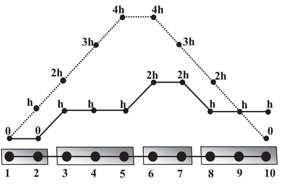
The Galerkin coarse-level correction (10) $\bm{\mathrm{e}}^{c}$ is the best approximation to a smooth error $\bm{\mathrm{e}}$ in the energy norm. Braess [6] noted that this does not guarantee a good approximation in the $l_{2}$ norm. For example, if $\bm{\mathrm{e}}$ is a piecewise linear function in a path graph (1-D grid with $w\equiv 1$) coarsened by aggregates of size two, $P\bm{\mathrm{e}}^{c}$ is constant on each aggregate and matches $\bm{\mathrm{e}}$’s slope across aggregates, resulting in about half the fine-level magnitude; cf. Fig. 5a.

An equivalent but more useful observation is that the energy of $\bm{\mathrm{P}}\bm{\mathrm{T}}\bm{\mathrm{e}}$ is twice larger than $\bm{\mathrm{e}}$’s, where $\bm{\mathrm{T}}\bm{\mathrm{e}}$ is a coarse representation of $\bm{\mathrm{e}}$, say,

$\bm{\mathrm{T}}$ is called the aggregate type operator (alternatively, $\bm{\mathrm{T}}\bm{\mathrm{e}}$ could be defined as the vector of seed values. Either definition satisfies $\bm{\mathrm{T}}\bm{\mathrm{P}}=\bm{\mathrm{I}}^{c}$ and falls under the umbrella of a corresponding CR theory [14, §2]). Rewrite (10) as

For an ideal interpolation $\bm{\mathrm{P}}$ that satisfies $\bm{\mathrm{P}}\bm{\mathrm{T}}\bm{\mathrm{e}}=\bm{\mathrm{e}}$, (18) is minimized by $\bm{\mathrm{y}}^{c}=\bm{\mathrm{T}}\bm{\mathrm{e}}$. A caliber-1 interpolation $\bm{\mathrm{P}}$ still satisfies $\bm{\mathrm{P}}\bm{\mathrm{T}}\bm{\mathrm{e}}\approx\bm{\mathrm{e}}$, but the first term in (18) is multiplied by the energy inflation factor

Now (18) is minimized by $\bm{\mathrm{y}}^{c}\approx q^{-1}\bm{\mathrm{T}}\bm{\mathrm{e}}$. As $\bm{\mathrm{e}}$ is not significantly changed by relaxation, its two-level ACF will be $\rho\approx 1-1/q$. In Fig. 5a, $q\approx 2$ and $\rho\approx.5$.

Several energy inflation remedies may be pursued:

• (A)

  Increase the interpolation’s caliber and accuracy. This leads to the fill-in troubles discussed in §2.

• (B)

  Accept an inferior two-level ACF of $1-1/q$ and increase the cycle index $\gamma$ to maintain it in a multilevel cycle. Unfortunately, not only does this increase complexity, the examples of §3.5.3 demonstrate that $q$ can be arbitrarily large. The ACF cannot be improved by additional smoothing steps either, because it is governed by smooth mode convergence.

• (C)

  Correct the coarse level operator $\bm{\mathrm{A}}^{c}$ to match the fine level operator’s energy during the setup phase.

• (D)

  Modify the coarse level correction $\bm{\mathrm{P}}\bm{\mathrm{e}}^{c}$ to match the fine level error $\bm{\mathrm{e}}$ during the solve phase.

In this section we consider option C. The Galerkin equation (11) is modified to

The key question is how to choose $\mu$. (Note that if $\mu$ is constant, Options C and D are equivalent.) Motivated by Fig. 5a and its two-dimensional analogue, Braess used $\mu=1.8$, but his V-cycle convergence for grid graphs was mesh-independent only if a fixed number of levels were used per cycle and if AMG was used as a PCG preconditioner. Moreover, no predetermined global factor exists that fits all error corrections in scenarios like Fig. 5b, because the coarse-level solution depends on local inflation ratios, which vary among graph nodes.

On the other hand, a local energy correction $\mu$ does exist. Indeed, the quadratic energies are separable to nodal energies

and define the local inflation factor as

In principle, a local $\mu_{U}$ can be designed using our TVs to at least partially offset $q_{U}$; unfortunately, new difficulties arise (cf. §5.3). Consequently, we chose to still scale all RHS entries by a flat $\mu$, but modify the aggregation so that $q_{U}(\bm{\mathrm{x}})\lessapprox Q$ for all smooth vectors $\bm{\mathrm{x}}$ and all $U\in\mathcal{N}^{c}$, where $Q>1$ is a parameter. Under this condition a global factor is effective, whose optimal value minimizes the overall convergence factor:

In our algorithm we set $Q=2$ and $\mu=\frac{4}{3}$. The expected smooth mode ACF is $Q/(Q+1)=\frac{1}{3}$.

Alternatively, a dynamic (flat or local) $\mu$ can be computed for scaling the correction $P\bm{\mathrm{e}}^{c}$ during the solve phase; see §3.6.1.

The local energy inflation varies considerably with aggregate size, shape and alignment. Consider the unweighted 2-D grid graph whose nodes are the 2-D coordinates $\{(i_{1},i_{2}):i_{1},i_{2}\in\mathbb{Z}\}$ in the plane $t_{1}$-$t_{2}$. Since all affinities are equal, the aggregation algorithm of may locally create archetype constellations such as Fig. 6a–d depending on node ordering during the aggregation stages.

Low-energy vectors $\bm{\mathrm{x}}$ are locally linear in $t_{1}$ and $t_{2}$, so their nodal values are modelled by $\bm{\mathrm{x}}(t_{1},t_{2})=a_{1}t_{1}+a_{2}t_{2}$. In Fig. 6a, the worst local energy ratio $Q$ at any aggregate, say $U=\{5,6\}$, is

References

- [1] P. R. Amestoy, T. A. Davis, and I. S. Duff, An approximate minimum degree ordering algorithm, SIAM J. Mat. Anal. Appl., 17 (1996), pp. 886–905.
- [2] R. Barrett, M. Berry, T. F. Chan, J. Demmel, J. Donato, J. Dongarra, V. Eijkhout, R. Pozo, C. Romine, and H. Van der Vorst, Templates for the Solution of Linear Systems: Building Blocks for Iterative Methods, 2nd Edition, SIAM, Philadelphia, PA, 1994.
- [3] M. Blatt, A parallel algebraic multigrid method for elliptic problems with highly discontinuous coefficients, PhD thesis, Universität Heidelberg, 2010.
- [4] E. G. Boman, B. Hendrickson, and S. Vavasis, Solving elliptic finite element systems in near-linear time with support preconditioners, SIAM J. Num. Anal., 46 (2008), pp. 3264–3284.
- [5] P. Borwein and T Erdélyi, Polynomials and Polynomial Inequalities, Springer-Verlag, New York, 1995.
- [6] D. Braess, Towards algebraic multigrid for elliptic problems of second order, Computing, 55 (1995), pp. 379–393.
- [7] A. Brandt, Rigorous quantitative analysis of multigrid, I. Constant coefficients two-level cycle with -norm, Siam J. Num Anal., 31 (1994).
- [8] , General highly accurate algebraic coarsening, J. Electron. Trans. Num. Anal., 10 (2000), pp. 1–20. Multilevel methods (Copper Mountain, CO, 1999).
- [9] , Multiscale scientific computation: Review 2001, in Multiscale and Multiresolution Methods, T. Barth, T. Chan, and R. Haimes, eds., Springer-Verlag, 2002, pp. 3–96.
- [10] A. Brandt, J. Brannick, K. Kahl, and I. Livshits, An algebraic distances measure of AMG strength of connection, ArXiv e-prints, (2011).
- [11] A. Brandt, J. Brannick, K. Kahl, and I. Livshits, Bootstrap amg, SIAM J. Sci. Comp., 33 (2011), pp. 612–632.
- [12] A. Brandt and O. E. Livne, Multigrid Techniques: 1984 Guide with Applications to Fluid Dynamics, Classics in Applied Mathematics, SIAM, revised ed., 2011.
- [13] A. Brandt, S. McCormick, and J. W. Ruge, Algebraic multigrid (AMG) for automatic multigrid solution with application to geodetic computations, tech. report, Colorado State University, Fort Collins, Colorado, 1983.
- [14] J. J. Brannick and R. D. Falgout, Compatible relaxation and coarsening in algebraic multigrid, SIAM J. Sci. Comp., 32 (2010), pp. 1393–1416.
- [15] M. Brezina, R. Falgout, S. MacLachlan, T. Manteuffel, S. McCormick, and J. Ruge, Adaptive smoothed aggregation (ASA), SIAM J. Sci. Comp., 25 (2004), p. 2004.
- [16] M. Brezina, P. Vanek, and P. S. Vassilevski, An improved convergence analysis of smoothed aggregation algebraic multigrid, Num. Lin. Alg. Appl., (2011).
- [17] H. Chang and D. Yeung, Graph laplacian kernels for object classification from a single example, in In CVPR (2, 2006, pp. 2011–2016.
- [18] F. R. K. Chung, Spectral Graph Theory (CBMS Regional Conference Series in Mathematics, No. 92), American Mathematical Society, Feb. 1997.
- [19] S. I. Daitch and D. A. Spielman, Faster approximate lossy generalized flow via interior point algorithms, CoRR, abs/0803.0988 (2008).
- [20] T. A. Davis, University of florida sparse matrix collection, NA Digest, 92 (1994).
- [21] DIMACS Center at Rutgers Univesity, Dimacs implementation challenges. Available online at http://dimacs.rutgers.edu/Challenges/, 2011.
- [22] C. H. Q. Ding, X. He, H. Zha, M. Gu, and H. D. Simon, A min-max cut algorithm for graph partitioning and data clustering, in Proceedings of ICDM 2001, 2001, pp. 107–114.
- [23] N.R. Draper and H. Smith, Applied Regression Analysis, Wiley-Interscience, 1998.
- [24] J. Ellson, E. R. Gansner, E. Koutsofios, S. C. North, and G. Woodhull, Graphviz - open source graph drawing tools, Graph Drawing, (2001), pp. 483–484.
- [25] R. Falgout, A. Cleary, J. Jones, E. Chow, V. Henson, C. Baldwin, P. Brown, P. Vassilevski, and U. Meier Yang, Hypre reference manual 2.7.0b. https://computation.llnl.gov/casc/hypre/download/hypre-2.7.0b_ref_manual.pdf, 2011.
- [26] P. Fischer, J. Lottes, D. Pointer, and A. Siegel, Petascale algorithms for reactor hydrodynamics, J. Physics: Conference Series, 125 (2008), p. 012076.
- [27] A. Frangioni and C. Gentile, Prim-based support-graph preconditioners for min-cost flow problems, Comput. Optim. Appl., 36 (2007), pp. 271–287.
- [28] J. R. Gilbert, C. Moler, and R. Schreiber, Sparse matrices in matlab: Design and implementation, SIAM J. Mat. Anal. Appl., 13 (1992), pp. 333–356.
- [29] G.H. Golub and C.F.V. Loan, Matrix Computations, Johns Hopkins studies in the mathematical sciences, Johns Hopkins University Press, third ed., 1996.
- [30] L. Gorelick, M. Galun, E. Sharon, R. Basri, and A. Brandt, Shape representation and classification using the poisson equation, in In In Proc. of CVPR04, 2004, pp. 61–67.
- [31] M. A. Heroux, R. A. Bartlett, V. E. Howle, R. J. Hoekstra, J. J. Hu, T. G. Kolda, R. B. Lehoucq, K. R. Long, R. P. Pawlowski, E. T. Phipps, A. G. Salinger, H. K. Thornquist, R. S. Tuminaro, J. M. Willenbring, A. Williams, and K. S. Stanley, An overview of the trilinos project, ACM Trans. Math. Softw., 31 (2005), pp. 397–423.
- [32] I. Koutis, G. L. Miller, and R. Peng, Approaching optimality for solving sdd linear systems, in Proceedings of the 2010 IEEE 51st Annual Symposium on Foundations of Computer Science, FOCS ’10, Washington, DC, USA, 2010, IEEE Computer Society, pp. 235–244.
- [33] D. Kushnir, M. Galun, and A. Brandt, Fast multiscale clustering and manifold identification, Pattern Recognition, 39 (2006), pp. 1876–1891.
- [34] , Efficient multilevel eigensolvers with applications to data analysis tasks, IEEE Transactions on Pattern Analysis and Machine Intelligence, 32 (2010), pp. 1377–1391.
- [35] Ann B. Lee, Diana Luca, Lambertus Klei, Bernie Devlin, and Kathryn Roeder, Discovering genetic ancestry using spectral graph theory, Genet. Epidem., 34 (2010), pp. 51–59.
- [36] O. E. Livne, Coarsening by compatible relaxation, Num. Lin. Alg. Appl., 11 (2004), pp. 205–227.
- [37] I. Livshits and A. Brandt, Accuracy properties of the wave-ray multigrid algorithm for helmholtz equations, SIAM J. on Sci. Comp., 28 (2006), pp. 1228–1251.
- [38] MathWorks, Creating C/C++ language mex-files. Available online at http://www.mathworks.com/help/techdoc/matlab_external/f7667.html, 2011.
- [39] L. N. Olson, J. B. Schroder, and R. S. Tuminaro, A general interpolation strategy for algebraic multigrid using energy minimization, SIAM J. Sci. Comp., 33 (2011), pp. 966–991.
- [40] D. Ron, I. Safro, and A. Brandt, Relaxation-based coarsening and multiscale graph organization, Multiscale Model. Sim., 9 (2011), pp. 407–423.
- [41] J. Ruge and K. Stüben, Algebraic multigrid (AMG), in Multigrid Methods, Frontiers in Applied Mathematics, S. F. McCormick, ed., SIAM, 1987, pp. 73–130.
- [42] I. Safro, Minimum logarithmic arrangement (MinLogA) results archive. Available online at http://www.mcs.anl.gov/~safro/mloga.html, 2011.
- [43] R. Sedgewick, Algorithms in C++, Part 5: Graph Algorithms, Addison-Wesley, 2002.
- [44] A. Sharma, R. P. Horaud, D. Knossow, and E. von Lavante, Mesh segmentation using laplacian eigenvectors and gaussian mixtures, in Proceedings of AAAI Fall Symposium on Manifold Learning and its Applications, Fall Symposium Series Technical Reports, Arlington, VA, November 2009, AAAI Press.
- [45] E. Sharon, M. Galun, D. Sharon, R. Basri, and A. Brandt, Hierarchy and adaptivity in segmenting visual scenes, Nature, 442 (2006), pp. 810–813.
- [46] D. A. Spielman, Algorithms, graph theory, and linear equations in laplacian matrices, in Proceedings of the International Congress of Mathematicians 2010 (ICM 2010), World Scientific, 2010, pp. 2698–2722.
- [47] D. A. Spielman and S. Teng, Nearly-linear time algorithms for preconditioning and solving symmetric, diagonally dominant linear systems, CoRR, abs/cs/0607105 (2006).
- [48] R. E. Tarjan, Depth first search and linear graph algorithms, SIAM J. Computing, 1 (1972), pp. 146–160.
- [49] W. F. Tinney and J. W. Walker, Direct solutions of sparse network equations by optimally ordered triangular factorization, Proc. IEEE, 55 (1967), pp. 1801–1809.
- [50] U. Trottenberg, C. W. Oosterlee, and A. Schüller, Multigrid, Academic Press, London, 2000.
- [51] C. Walshaw, Multilevel refinement for combinatorial optimisation problems, Annals Oper. Res., 131 (2004), pp. 325–372.
- [52] F. Zhang, The Schur Complement And Its Applications (numerical Methods And Algorithms), Springer-Verlag, 2005.
- [53] X. Zhu, Z. Ghahramani, and J. D. Lafferty, Semi-supervised learning using Gaussian fields and harmonic functions., in ICML’03, 2003, pp. 912–919.