Splitting of degenerate states in one-dimensional quantum mechanics
Abstract
A classic “no-go” theorem in one-dimensional quantum mechanics can be evaded when the potentials are unbounded below, thus allowing for novel parity-paired degenerate energy bound states. We numerically determine the spectrum of one such potential and study the parametric variation of the transition wavelength between a bound state lying inside the valley of the potential and another, von Neumann-Wigner-like state, appearing above the potential maximum. We then construct a modified potential which is bounded below except when a parameter is tuned to vanish. We show how the spacing between certain energy levels gradually decrease as we tune the parameter to approach the value for which unboundedness arises, thus quantitatively linking the closeness of degeneracy to the steepness of the potential. Our results are generic to a large class of such potentials. Apart from their conceptual interest, such potentials might be realisable in mesoscopic systems thus allowing for the experimental study of the novel states. The numerical spectrum in this study is determined using the asymptotic iteration method which we briefly review.
I Introduction
Bound states in quantum mechanical potential problems usually have energies below the potential maximum, as most quantum mechanics textbooks remind us. However, already in 1929 von Neumann and Wigner [1] first noted the theoretical existence of a class potentials which support normalizable bound states above the potential maximum, embedded in the continuum of scattering states. Later work by Stillinger and Herrick [2] provided a more detailed understanding of such unusual bound states, indicating their essential quantum mechanical nature. The von Neumann–Wigner above–barrier bound states, were eventually experimentally verified in the 1990s, by Capasso et al. [3], through observations on allowed transitions, between a state inside the valley and another above the potential maximum, in semiconductor heterostructures.
Recently, potentials unbounded from below, in one dimension, have attracted interest because of certain unusual features in their energy eigenvalues and eigenfunctions. The class of potentials studied were non-singular in any finite domain but asymptotically approached negative infinity. It was shown that such potentials not only have von Neumann–Wigner states, they also exhibit a new feature: parity-paired degenerate bound states with real energies [5, 4], a property prohibited for regular one-dimensional potentials [6]. The study of such potentials is thus conceptually interesting as they highlight how commonly accepted “no-go” theorems may be evaded.
It should also be noted that such unbounded-below potentials are not just mathematical constructs, but have appeared in the context of localization of fields on the 3–brane in the study of the so-called braneworld models with warped extra dimensions in high energy physics[7]. As mentioned in [4], and discussed below, such potentials might be realisable, to any given degree of accuracy, in actual mesoscopic systems.
In this paper, we study in detail the spectrum of two potentials so as to anticipate future experimental investigations as suggested in Ref.[4]. We first numerically compute the eigenvalues, and hence transition wavelengths, for the cosh-sech potential to supplement the partial information that is available in earlier analytical work [4].
We then modify the unbounded potential in such a way that the unboundedness appears only when we tune a parameter in the potential to vanish. This allows us to study how the degenerate states of the unbounded potential split as the parameter is varied, and as one moves to the more realistic bounded potential. Since in [4] we had shown the existence of large classes of potentials supporting degenerate bound states, the splitting of the degenerate states for the bound versions of those potentials is naturally expected and thus our results are qualitatively generic.
The eigenvalues are determined with the help of the asymptotic iteration method (AIM), a relatively novel technique to solve second-order linear homogeneous differential equations with variable coefficients [8, 9, 10, 11, 12] (details of the method are provided in Appendix A). Its asset is that it is able to easily circumvent some of the profound analytical and numerical difficulties posed for the Schrödinger equation with potentials which are either singular or unbounded from below.
Our article is organised as follows. In Section II, we discuss the cosh-sech potential and determine its spectrum using the asymptotic iteration method (AIM). In Section III we discuss the degeneracy of states and how the levels split in the modified bounded potential that we construct. Section IV summarises our results while the appendices (Appendix A and Appendix B) contain some technical details about AIM and physical units, respectively.
II A modified Pösch–Teller potential
Consider the cosh-sech potential,
| (1) |
This differs from the potential studied in [13] just by an additive constant, , since they [13] choose the first term as a function.
The above potential has a maximum at
which exists only for since . The extrema of the potential function are and The potential is of the same form as the volcano potential of Ref. [5],
| (2) |
with , which can be generated from the general ansatz of Ref. [4] by choosing .
To solve the time–independent Schrodinger equation using the AIM (see Appendix A), the wave function is written as [13], where
| (3) |
A further change of independent variable to , transforms the Schrodinger equation to
| (4) |
where
| (5) |
| (6) |
The above form of the Schrodinger equation is necessary in order to use AIM, to find energy eigenvalues for different values.
II.1 Energy spectra and transition wavelengths
We now present the results of our calculations using the asymptotic iteration method. All computations were carried out using standard routines in Mathematica with default precision.
In Fig. 1, we plot the dimensionless energy eigenvalues (see Appendix B for a discussion on physical units) for the unbounded potential with and varying from up to . One can observe that for energy eigenvalues, as increases, energies increase in general. Our calculations (not shown here) also show that the energy eigenvalues monotonically decrease with the value of the parameter .

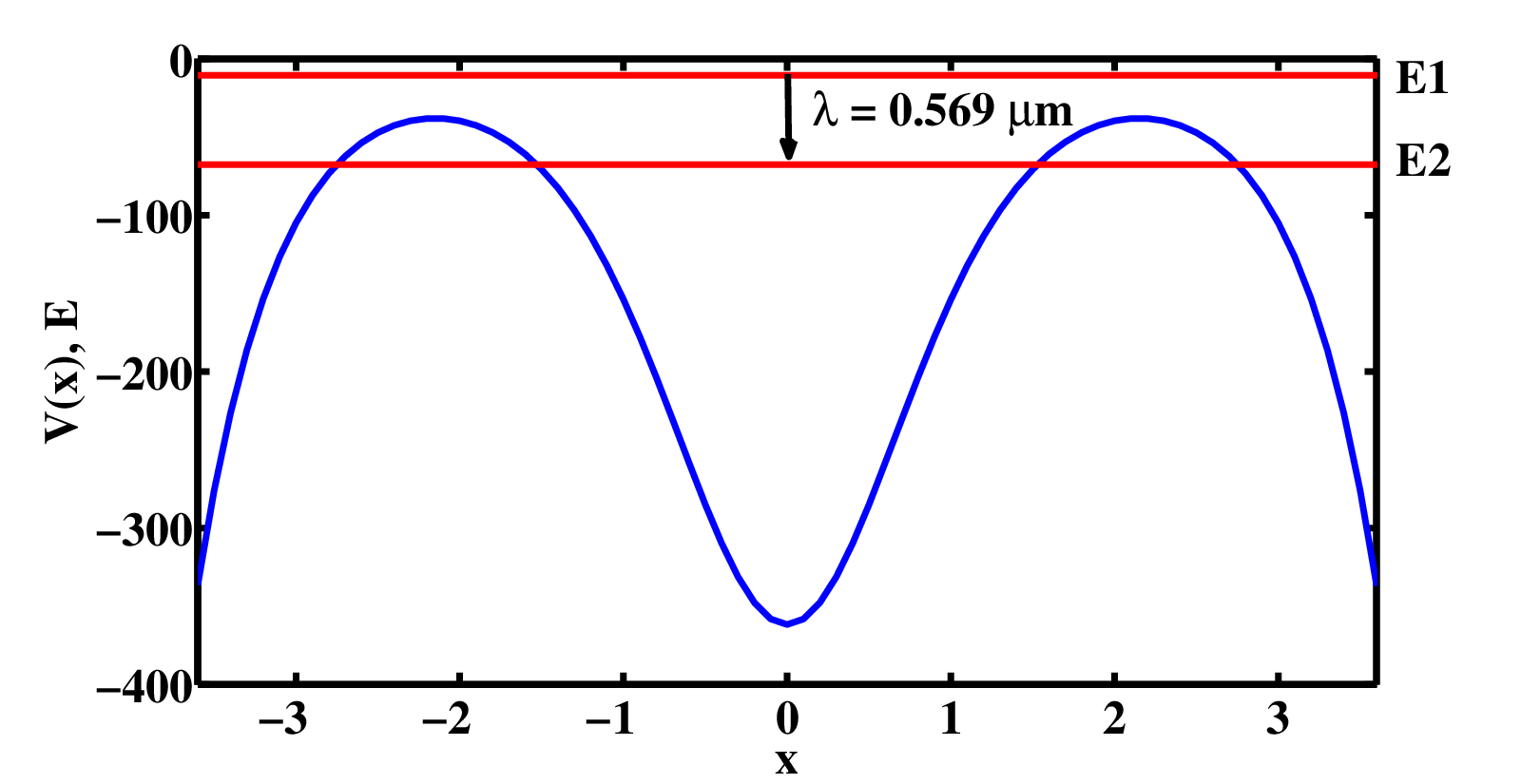


The transition wavelength between a pair of states can be determined from the difference in their energies, after converting to suitable physical units, as outlined in Appendix B. Fig. 2 demonstrates a pair of eigenstates located above (E1) and below (E2) the maximum in the potential well. The parameters and of the cosh-sech potential have been chosen so that the transition wavelength lies in the visible range of the electromagnetic spectrum.
The transition wavelength can be varied over the range of interest by modifying the parameters and ; from Fig. 3, it is evident that for to 16, is in the IR region, and greater values of lead to transitions in the visible region. Similarly, Fig. 4 shows a variation of the transition wavelength from the IR to the ultra-violet region by changing the parameter . Note that since the energy differences increase with an increase in , hence moves from the longer IR wavelengths to the relatively short visible region.
For illustration, the length scale parameter (see Appendix B) had been chosen to be 10 in the above calculations. can be modified suitably to obtain orders of magnitude variation in the energy eigenvalues (in physical units) and the corresponding transition wavelengths.
III Degeneracy
As mentioned earlier, a curious feature of the class of unbounded potentials being considered here is the existence of degeneracy of the bound eigenstates despite the fact that we are dealing with one-dimensional quantum mechanical problems [5, 4]. Not all potentials unbounded from below as support degenerate bound states; for instance the quartic anharmonic oscillator with , is not known to exhibit degeneracy.
Here we show, numerically, that the degeneracy exists in our potential for many excited states which lie above the previously analytically obtained pair of states (possibly ground states) in Ref.[4].
Consider the cosh-sech potential with . After 12 iterations, the following eigenvalues are obtained using the AIM: . It can be inferred that the energy eigenvalues occur in closely separated pairs. Moreover, the separation between the two eigenvalues in a pair keeps on decreasing with an increase in the number of iterations, suggesting that they are ideally degenerate. The energy eigenvalues below the minimum in at do not correspond to bound states. This is discussed in [14] (see also [13]), where the authors show how the below-minimum states are not linked to total–transmission (TT) modes, unlike genuine bound states which are always constructed out of the TT modes. Further, we have also seen that these below-minimum states do not occur in pairs, a feature different from the above-minimum bound states. Thus, in all our evaluations using AIM we have ignored such states.
Next, we consider a modified potential which diminishes to zero instead of going to infinity as , and which should be realisable in a laboratory. We multiply the cosh term in Eq.1, which is responsible for the unboundedness, by an exponentially decaying term controlled by the parameter .
| (7) |
The original potential can be recovered by setting . As increases, the first term gets suppressed, and the potential retreats to zero at a faster rate. This effect is illustrated in the Fig. 5 for . For , the behaviour of is quite close to that for near the origin, but far from , the potential decays to zero instead of the latter case which goes to . This offers promise in investigating the relationship between unboundedness and degeneracy. On the other hand, the case is similar to the bounded potential well or the Pösch-Teller potential rather than the unbounded cosh-sech potential. Thus, can be used to tune the steepness of the potential away from the origin.

The energy spectrum of the modified potential can be obtained via the AIM by changing the expression for in Eq. 6 to:
| (8) |
The factor occurs in the exponent due to the intermediate variable transformation .
Fig. 6 shows the energy eigenvalues of the pair of degenerate states with the parameter for the specific case of the potential considered above (viz. ). As we have seen before, a bound state exists for the unbounded potential at -0.25. It is evident from the plot that the pair of degenerate levels splits into separate levels with an increase in . The splitting is also shown separately in Fig. 7 where the energy difference is plotted. We note that as we move towards the left (i.e. ), the minute difference between the two degenerate eigenvalues which still remain even at , is due to numerical error in the AIM rather than actual splitting. This is why the curve is steadily increasing for and flattens for . In fact, does not go below even for , if we use 12 iterations.

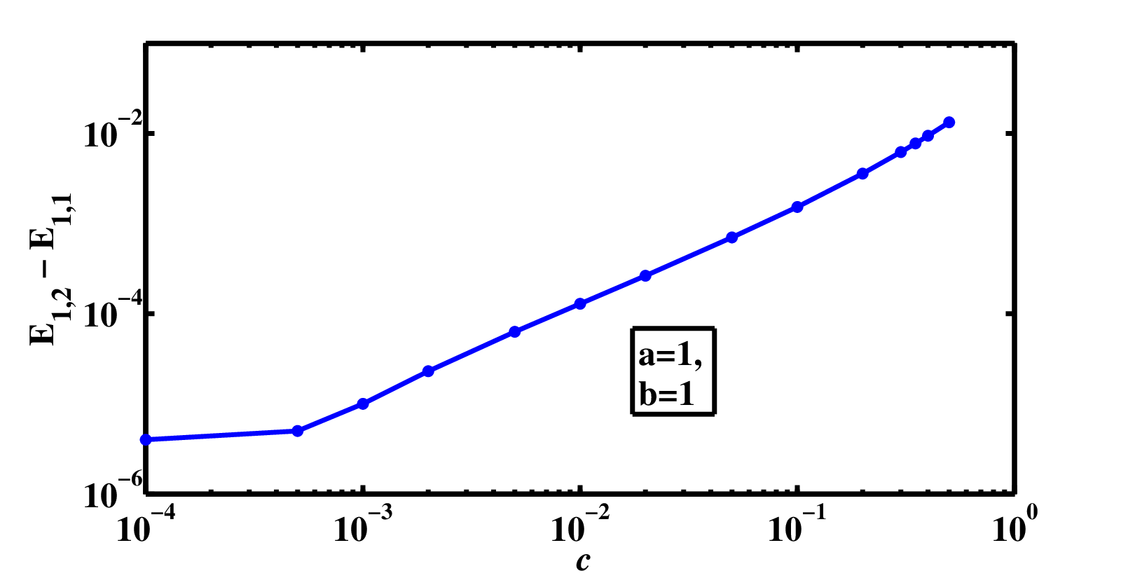
Thus, tuning the parameter modifies the potential from an unbounded to a bounded one, and gradually increases the separation between the levels which are degenerate in the unbounded case. While it might be impossible to physically realize the unbounded potential (), its variants such as the potentials with can be experimentally fabricated through methods of band-gap engineering in semiconductor heterostructures [15], where potentials with multiple wells and barriers do arise and are not very uncommon. The experimental energy eigenvalues can thus be compared with the theoretically predicted results with the help of measured transition wavelengths.
IV Conclusion
In this paper we first calculated the energy spectra and transition wavelengths between states with energies lying within the potential valley and above the potential maximum for the volcano potential (1), thus extending in detail the analytically obtained results in [4].
We emphasize that we have been able to demonstrate, through our numerical work in this paper, that there exist several degenerate excited states in the full spectrum, beyond the single pair obtained analytically in Ref.[4]. We then constructed a new potential, depending on a tunable parameter , which was similar to the volcano potential near the origin but which was bounded as for . This non-singular potential exhibited non–degenerate energy eigenvalues. For one has the original volcano potential with degenerate states and as is increased, creating a bounded potential, the splitting of degenerate states also increased.
As stated in Section I, the properties of the bounded potential we studied here are likely to be qualitatively similar to others that can be constructed from the general ansatz of Ref.[4] and plausibly amenable to experimental realization in semiconductor heterostructures. We believe that laboratory fabrication of systems where such potentials may arise could be a route to the observation of the novel parity paired (almost) degenerate states in such one-dimensional problems. Further, the splitting of the degeneracy will lead to tunable (varying ) long wavelength transitions between the closely spaced split levels for the bounded potential. As for the case of the von Neumann-Wigner states, we feel that the study of such parity-paired degenerate states is of intrinsic conceptual interest.
Finally, the present study once again shows that the AIM is a useful semi-analytical tool to solve Scrödinger-type eigenvalue problems. We have verified the pre-existing bound state analytical solutions for unbounded potentials, with the help of the AIM, and extended the method to determine the entire bound state energy spectrum of these potentials which are unbounded below.
Appendix A: The asymptotic iteration method
The asymptotic iteration method (AIM) [8] is a general semi-analytical technique for solving second order, linear homogeneous ordinary differential equations (ODEs). It has been used quite extensively over the last few years, in a variety of contexts (see [10, 11, 12] for a few references). The basic idea behind the method is as follows. Let and be functions defined over a certain interval, having appropriately many successive derivatives. The differential equation we are concerned with is given as
| (9) |
This equation is to be solved by the AIM. The technique consists of iteratively differentiating the equation to obtain an ODE of the same general type, where the coefficients of the next step are related to the previous coefficients by the expressions
| (10) | |||||
| (11) |
The iteration is terminated when the ratio between the coefficients becomes independent of the index ,
| (12) |
in which case the equation is exactly solvable with the help of the AIM and exact eigenvalues are obtained by finding the roots of the discriminant equation
| (13) |
On the other hand, if the ratio of succesive coefficients is not strictly independent of , exact solutions cannot be found by the AIM. Nonetheless, an approximation to the eigenvalues can be obtained by forced imposition of the condition in Eq. 12 for a sufficiently large value of , wherein lies the asymptotic nature of the method.
Furthermore, after some algebra, it is shown in [8] that the solution to Eq. 9 can be obtained by the following integral relation:
| (14) |
The time independent Schrödinger equation is of the form
| (15) |
By a suitable transformation of which reflects the asymptotic behaviour of the wave function, Eq. 15 can be recast into a form resembling Eq. 9, where and depend on the energy . Applying the asymptotic iteration method, the ’s and ’s are determined to arrive at the “quantization” condition of Eq. 13. Since depends on both and , it becomes necessary to choose a suitable value of in order to solve for the energy eigenvalue . For exactly solvable models, an arbitrary choice of suffices to arrive at the correct eigenvalue. On the contrary, for models which are not exactly solvable, the choice of affects the rate of convergence of the method, and hence the accuracy of the energy calculated.
It is noteworthy that the AIM is essentially an analytical technique, as the successive derivatives required are determined by analytic or symbolic differentiation. However, the form of is usually so complicated that the use of numerical algorithms is necessary in order to calculate the roots of the equation , with a choice of where is usually taken to be the critical (maximum/minimum) point of the potential.
We tested the AIM on the potentials mentioned in [4] and verified that the numerical eigenvalues agree with the partial information already available analytically. For example, we have checked that for there is always one energy eigenvalue , which corresponds to the known exact solution [4]. New results are presented in the main body of this paper.
Appendix B: Physical units
In dimensionless (atomic) units, the time independent Schrödinger equation is:
| (16) |
where is a dimensionless variable proportional to the one-dimensional spatial coordinate and is the potential proportional to that in the actual quantum mechanical problem.
On the other hand, the Schrödinger equation in real units is:
| (17) |
The dimensionless coordinate can be related to the dimensional coordinate with the help of a length scale parameter , . Here, is a measure of the width of the potential. Substituting this relation in Eq. 17, we get:
| (18) |
Comparing with Eq. 16,
| (19) |
Thus, we have,
| (20) |
For example, an electron with a mass has an energy:
| (21) | |||||
If we take , the dimensionless energy is related to the real energy by the factor,
| (22) |
Corresponding to an energy difference , the transition wavelength . As an example, consider the red and violet ends of the visible spectrum corresponding to wavelengths of 0.8 and 0.4 , which translate to dimensionless energy differences of 81.51 and 40.75 respectively. By suitable choice of the parameters in the potentials, it is possible to obtain transition wavelengths in the optical range or beyond.
References
- [1] J. von Neumann and E. Wigner, Phys. Z. 30, 465 (1929).
- [2] F. H. Stillinger and D. R. Herrick, Phys. Rev. A 11, 446 (1975).
- [3] F. Capasso, C. Sirtori, J. Faist, D. L. Sivco, S. N. G. Chu, A. Y. Cho, Nature 358, 565 (1992).
- [4] S. Kar and R. Parwani, Europhys. Lett. 80, 30004 (2007).
- [5] R. Koley and S. Kar, Phys. Lett. A 363, 369(2007).
- [6] L. Landau and E. M. Lifshitz, Quantum Mechanics (Pergamom Press, Oxford), 1977, p. 60.
- [7] L. Randall and R. Sundrum, Phys. Rev. Lett. 83, 4690 (1999).
- [8] H. Ciftci, R. L. Hall and N. Saad, J. Phys. A: Math. Gen. 36, 11807 (2003)
- [9] F. M. Fernandez, J. Phys. A: Math. Gen. 37, 6173 (2004).
- [10] H-T. Cho, A. S. Cornell, J. Doukas and W. Naylor, Phys. Rev. D 80, 064022 (2009)
- [11] H-T. Cho, A. S. Cornell, J. Doukas and W. Naylor, Class. Qtm. Grav. 27, 155004 (2010)
- [12] R. L. Hall, N. Saad and K. D. Sen, J. Phys. A: Math. Theor. 44, 185307 (2011).
- [13] A. J. Sous, M. I. El-Kawni, Int. J. Mod. Phys. A 24, 4169 (2009).
- [14] H-T. Cho and C-L Ho, J. Phys. A: Math. Theor. 41, 172002 (2008).
- [15] F. Capasso, J. Faist and C. Sirtori, J. Math. Phys. 37, 4775 (1996).