A-polynomial, B-model, and Quantization

The starting point of the topological recursion [12] is the choice⁴⁴ 4 As will be explained in section 2.3, this choice is related to the choice of polarization. of a parametrization, i.e. a choice of two functions of a local variable $p$,

$$\left\{\begin{array}[]{l}u=u(p)\\ v=v(p)\end{array}\right.$$

(19)

where $u(p)$ is assumed to have non-degenerate critical points. (In particular, for curves of genus zero, both $u(p)$ and $v(p)$ can be rational functions. We are not going to assume this, however, and, unless noted otherwise, much of our discussion below applies to curves of arbitrary genus.) Then, from this data alone one can recursively determine the perturbative coefficients $S_{n}$ of the partition function (11) via a systematic procedure that we explain below.

For example, as we already noted in (18) the leading term $S_{0}$ is obtained by integrating a 1-form differential $\phi=vdu$ along a path on the curve $A(u,v)=0$. When expressed in terms of the local coordinate $p$, this integral looks like

$$S_{0}\;=\;\int^{p}\phi=\int^{p}v(p)du(p)\,,$$

(20)

and sometimes is also referred to as the anti-derivative of $\phi$. Then, the next-to-the-leading term $S_{1}$ is determined by the two-point function, or the so-called annulus amplitude. For a curve ${\cal C}$ of genus zero it can be expressed in terms of the parametrization data (19) by the following formula⁵⁵ 5 Notice, our prescription here and also in eq. (23) differs from that in [15]. As will be explained below, these differences are important for overcoming the obstacles in [15] and reproducing the “quantum” $q$-corrections in the quantization of the $A$-polynomial (17).

$$S_{1}\;=\;-\frac{1}{2}\log\frac{du}{dp}\,,$$

(21)

whose origin and generalization to curves of arbitrary genus will be discussed in section 2.5. We recall that, according to (14), the term $S_{1}$ contains information about the “torsion” $T(u)$ and generically is all one needs in order to determine the quantum curve $\widehat{A}$ when it has a nice polynomial form (15).

In a similar manner, the topological recursion of Eynard-Orantin [12] can be used to determine all the other higher-order terms $S_{n}$, $n\geq 2$. Starting with the parametrization (19), one first defines a set of symmetric degree-$n$ meromorphic differential forms $W^{g}_{n}=W^{g}_{n}(p_{1},p_{2},\ldots,p_{n})$ on ${\cal C}^{n}$ via a systematic procedure that we shall review in a moment. Then, by taking suitable integrals and residues one obtains respectively the desired $S_{n}$’s, as well as their “closed string” analogs known as the genus-$g$ free energies $F_{g}$:

$$\boxed{\phantom{\int}\begin{array}[]{c@{\qquad}c@{\qquad}c@{\qquad}c@{\qquad}c}\text{$u(p)$ ~and~ $v(p)$}&\leadsto&\text{$W^{g}_{n}$}&\leadsto&\text{$S_{n}$ ~and~ $F_{g}$}\end{array}\phantom{\int}}$$

(22)

Specifically, motivated by the form of a determinant in (12), or a definition of the Baker-Akhiezer function in [12, 16, 17], we construct $S_{n}$’s as the following linear combinations of the integrated multilinear meromorphic differentials:

$$S_{n}(p)=\sum_{2g-1+k=n}\frac{1}{k!}\,\underbrace{\int^{p}_{\tilde{p}}\cdots\int^{p}_{\tilde{p}}}_{\text{$k$ times}}\,W^{g}_{k}(p^{\prime}_{1},\ldots,p^{\prime}_{k})\,,$$

(23)

where each differential form $W^{g}_{k}$ of degree $k$ is integrated $k$ times.⁶⁶ 6 For curves of genus one or higher one should consider more general Baker-Akhiezer function, which in addition includes non-perturbative corrections represented by certain $\theta$-functions [16]. As the examples which we consider concern mostly curves of genus zero, we do not analyse such corrections explicitly. The base point of integration $\tilde{p}$ is chosen such that $u(\tilde{p})\to\infty$ [17]. In turn, the multilinear differentials $W^{g}_{n}$ are obtained by taking certain residues around critical points of the “Morse function” $u(p)$, i.e. solutions to the equations

$$du(p)|_{p^{*}_{i}}=0\qquad\Leftrightarrow\qquad\partial_{v}A|_{p^{*}_{i}}=0\,,$$

(24)

where the standard shorthand notation $\partial_{v}\equiv\frac{\partial}{\partial v}$ is used. Following [12], we shall refer to these points as the “branch points” of the curve ${\cal C}$ in parametrization (19). We assume that all branch points are simple (or, as sometimes referred to, regular), i.e. for each point $p$ in the neighborhood of a branch point $p^{*}_{i}$ there is a unique, conjugate point $\bar{p}$, such that

$$u(p)\;=\;u(\bar{p})\,.$$

(25)

The next essential ingredient for the topological recursion is the differential 1-form⁷⁷ 7 For reasons that will become clear later, we choose a sign opposite to the conventions of [12]. called the “vertex”:

	$\displaystyle\omega(p)$	$\displaystyle=$	$\displaystyle\big(v(\bar{p})-v(p)\big)du(p)\,\,\,\,\,\,\,\,\qquad\qquad{\rm~for~curves~in~}{\mathbb{C}}\times{\mathbb{C}}\,,$		(26)
		$\displaystyle=$	$\displaystyle\big(\log y(\bar{p})-\log y(p)\big)\frac{dx(p)}{x(p)}\qquad{\rm~for~curves~in~}{\mathbb{C}}^{*}\times{\mathbb{C}}^{*}\,,$

and the 2-form $B(p,q)$ known as the Bergman kernel. The Bergman kernel $B(p,q)$ is defined as the unique meromorphic differential with exactly one pole, which is a double pole at $p=q$ with no residue, and with vanishing integral over $A_{I}$-cycles $\oint_{A_{I}}B(p,q)=0$ (in a canonical basis of cycles $(A_{I},B^{I})$ for ${\cal C}$). Thus, for curves of genus zero the Bergman kernel takes a particularly simple form

$$B(p,q)\;=\;\frac{dp\,dq}{(p-q)^{2}}\,,$$

(27)

and its form for curves of higher genus is presented in section 2.5. A closely related quantity is a 1-form, defined in a neighborhood of a branch point $q^{*}_{i}$

$$dE_{q}(p)\;=\;\frac{1}{2}\int_{q}^{\bar{q}}B(\xi,p)\,.$$

Finally, the last important ingredient is the recursion kernel $K(q,p)$,

$$K(q,p)\;=\;\frac{dE_{q}(p)}{\omega(q)}\,.$$

(28)

Having defined the above ingredients we can present the recursion itself. When expressed in variables $(u,v)$, the recursion has the same form for curves in ${\mathbb{C}}\times{\mathbb{C}}$ as it does for curves in ${\mathbb{C}}^{*}\times{\mathbb{C}}^{*}$. It determines higher-degree meromorphic differentials $W^{g}_{n}(p_{1},\ldots,p_{n})$ from those of lower degree. The initial data for the recursion are one- and two-point correlators of genus zero, the former vanishing by definition and the latter given by the Bergman kernel:

		$\displaystyle:\qquad$	$\displaystyle W^{0}_{1}(p)\;=\;0\,,$		(29)
		$\displaystyle:\qquad$	$\displaystyle W^{0}_{2}(p_{1},p_{2})\;=\;B(p_{1},p_{2})\,.$		(30)

It is also understood that $W^{g<0}_{n}=0$.

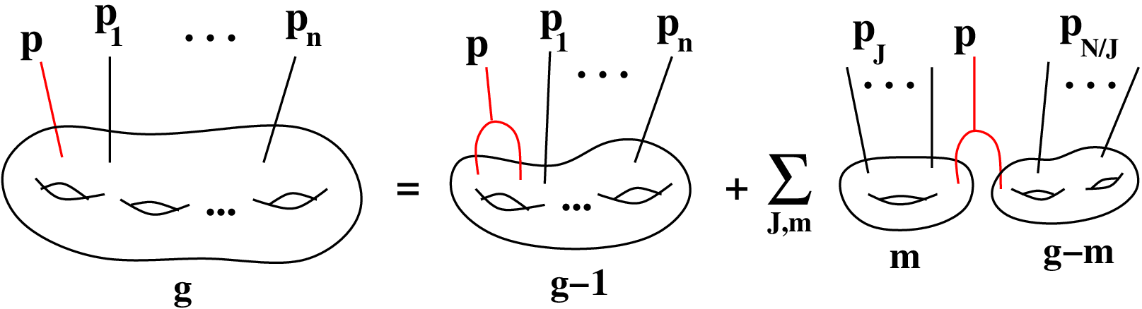
The other differentials are defined recursively as follows. For a set of indices $J$ denote $\vec{p}_{J}=\{p_{i}\}_{i\in J}$. Then, for $N=\{1,\ldots,n\}$ and the corresponding set of points $\vec{p}_{N}=\{p_{1},\ldots,p_{n}\}$ define

	$\displaystyle{\raisebox{-17.07182pt}{\includegraphics[width=56.9055pt]{recursion1}}\,}:\quad W^{g}_{n+1}(p,\vec{p}_{N})$	$\displaystyle=$	$\displaystyle\sum_{q^{*}_{i}}\textrm{Res}_{q\to q^{*}_{i}}K(q,p)\Big(W^{g-1}_{n+2}(q,\bar{q},\vec{p}_{N})+$		(31)
			$\displaystyle+\sum_{m=0}^{g}\sum_{J\subset N}W^{m}_{|J|+1}(q,\vec{p}_{J})W^{g-m}_{n-|J|+1}(\bar{q},\vec{p}_{N/J}\Big),$

where $\sum_{J\subset N}$ denotes a sum over all subsets $J$ of $N$, cf. Figure 1. These correlators have many interesting properties. For example, any $W^{g}_{n}(p_{1},\ldots,p_{n})$ is a symmetric function of $p_{i}$. Furthermore, apart from the special case of $g=0$ and $n=2$, the poles of $W^{g}_{n}(p_{1},\ldots,p_{n})$ in variables $p_{i}$ appear only at the branch points. In addition, the $A_{I}$-cycle integrals with respect to any $p_{i}$ vanish, $\oint_{p_{i}\in A_{I}}W^{g}_{n}(p_{1},\ldots,p_{n})=0$. For a detailed discussion of these and many other features of $W^{g}_{n}$ see [12].

Let us briefly illustrate how the recursion procedure works. First, from the recursion kernel (28) and from the Bergman kernel (30) one finds the genus-1 one-point correlator

$$W^{1}_{1}(p)\;=\;\sum_{q^{*}_{i}}\textrm{Res}_{q\to q^{*}_{i}}K(q,p)W^{0}_{2}(q,\bar{q})\,.$$

(32)

Then, the following series (with $g+n=3$) is determined

	$\displaystyle W^{0}_{3}(p,p_{1},p_{2})$	$\displaystyle=$			(33)
		$\displaystyle=$	$\displaystyle\sum_{q^{*}_{i}}\textrm{Res}_{q\to q^{*}_{i}}K(q,p)\Big(W^{0}_{2}(q,p_{1})W^{0}_{2}(\bar{q},p_{2})+W^{0}_{2}(\bar{q},p_{1})W^{0}_{2}(q,p_{2})\Big)\,,$
	$\displaystyle W^{1}_{2}(p,p_{1})$	$\displaystyle=$	$\displaystyle{\,\raisebox{-8.5359pt}{\includegraphics[width=22.76228pt]{recursion7}}\,}=\sum_{q^{*}_{i}}\textrm{Res}_{q\to q^{*}_{i}}K(q,p)\Big(W^{0}_{3}(q,\bar{q},p_{1})+2W^{1}_{1}(q)W^{0}_{2}(\bar{q},p_{1})\Big)\,,$		(34)
	$\displaystyle W^{2}_{1}(p)$	$\displaystyle=$	$\displaystyle{\,\raisebox{-8.5359pt}{\includegraphics[width=31.2982pt]{recursion6}}\,}=\sum_{q^{*}_{i}}\textrm{Res}_{q\to q^{*}_{i}}K(q,p)\Big(W^{1}_{2}(q,\bar{q})+W^{1}_{1}(q)W^{1}_{1}(\bar{q})\Big)\,.$		(35)

Next, one finds a series $W^{0}_{4},W^{1}_{3},W^{2}_{2},W^{3}_{1}$ with $g+n=4$, and so on. In the end, from each such series one can determine one more $S_{n}$ using (23). For example, as will be discussed in section 2.5, $S_{1}$ is obtained by integrating the Bergman kernel:

$$S_{1}(p)\;=\;\frac{1}{2}\lim_{p_{1}\to p_{2}=p}\int\left(B(p_{1},p_{2})-\frac{du(p_{1})\,du(p_{2})}{(u(p_{1})-u(p_{2}))^{2}}\right)\,,$$

(36)

and for curves of genus zero this formula reproduces the expression (21) proposed earlier. At the next step, from the series of the multilinear differentials (33) - (35) one finds the next term in the perturbative series (11):

$$S_{2}(p)\;=\;\int^{p}_{\tilde{p}}W^{1}_{1}(p_{1})+\frac{1}{3!}\int^{p}_{\tilde{p}}\int^{p}_{\tilde{p}}\int^{p}_{\tilde{p}}W^{0}_{3}(p_{1},p_{2},p_{3})\,,$$

(37)

and so on. As noted before, the base point of integration $\tilde{p}$ is chosen such that $u(\tilde{p})\to\infty$ [17].

While not of our immediate concern in this paper, for completeness we also recall a definition of genus-$g$ free energies $F_{g}$. For $g\geq 2$ they come⁸⁸ 8 Notice, compared to the conventions of [12] we introduce an extra minus sign in our definition of $F_{g}$ in order to account for the sign of $W^{g}_{1}$ originating from the sign in (26). from the corresponding $W^{g}_{1}$:

$$F_{g}\;=\;\frac{1}{2g-2}\sum_{q^{*}_{i}}\textrm{Res}_{q\to q^{*}_{i}}S_{0}(q)W^{g}_{1}(q)\,,$$

(38)

where $S_{0}(q)=\int^{q}v(p)du(p)$, while $F_{0}$ and $F_{1}$ are defined independently in a more intricate way presented in [12]. Among various interesting properties of $F_{g}$ the most important one is their invariance under symplectic transformations of the spectral curve.

Finally, since the relation between $S_{n}$ and $W^{g}_{k}$ will be crucial for computing $\widehat{A}$ from the classical curve $A=0$ and its parametrization, let us briefly explain our motivation behind (23). Recall, that the correlators $W^{g}_{k}(p_{1},\ldots,p_{k})$ in (23) were originally introduced [12] in a way which generalizes and, when an underlying matrix model exists, reproduces connected contributions to the matrix model expectation value

$$\Big\langle\textrm{Tr}\Big(\frac{1}{u(p_{1})-M}\Big)\cdots\textrm{Tr}\Big(\frac{1}{u(p_{k})-M}\Big)\Big\rangle_{{\rm conn}}=\sum_{g=0}^{\infty}\hbar^{2g-2+k}\frac{W^{g}_{k}(p_{1},\ldots,p_{k})}{du(p_{1})\ldots du(p_{k})}$$

in an ensemble of matrices $M$ of size $N=\hbar^{-1}$.⁹⁹ 9 Strictly speaking, this equation holds for $k>2$ and there are some corrections to the lowest order terms with $k=1$ and $k=2$ [12]. Integrating both sides with respect to all variables and then setting $p_{1}=\ldots=p_{k}=p$, we get

$$\Big\langle\Big(\textrm{Tr}\log\big(u(p)-M\big)\Big)^{k}\Big\rangle_{{\rm conn}}=\sum_{g=0}^{\infty}\hbar^{2g-2+k}\int^{p}\cdots\int^{p}W^{g}_{k}(p_{1}^{\prime},\ldots,p_{k}^{\prime}).$$

Dividing both sides by $k!$ and summing over $k$ we get

$$\Big\langle\,\textrm{det}(u-M)\,\Big\rangle_{{\rm conn}}=\sum_{n=0}^{\infty}\hbar^{n-1}S_{n}(p),$$

with $S_{n}(p)$ defined in (23). Whereas the left hand side represents the connected expectation value, the right hand side plays the role of the free energy, so that

$$Z=\Big\langle\,\textrm{det}(u-M)\,\Big\rangle=e^{\frac{1}{\hbar}\sum_{g=0}^{\infty}\hbar^{n}S_{n}(p)}.$$

This result is in agreement with (11) and (12) and provides the motivation for the definition (23). From the matrix model point of view, the free energies $F_{g}$ defined in (38) encode the total partition function

$$\langle 1\rangle=\int\mathcal{D}Me^{-\frac{1}{\hbar}\textrm{Tr}V(M)}=e^{\sum_{g=0}^{\infty}\hbar^{2g-2}F_{g}}\,.$$

(39)

From a string theory viewpoint, this partition function would correspond to closed string amplitudes. In fact, in many instances relevant to Seiberg-Witten theory or topological strings, matrix models which encode corresponding partition functions (39) have been explicitly constructed in [18, 19, 20, 21, 22, 23, 24].

Our next goal is to compare the results of the topological recursion to the structure of the “quantum curve”

$$\widehat{A}\;\simeq\;0\,,$$

(40)

where we used a shorthand notation “$\simeq$” to write (10) in a form that makes a connection with its classical limit $A(x,y)=0$ manifest, cf. [25]. In general, the Schrödinger-like equation (10) and its abbreviated form (40) is either a $q$-difference equation (for curves in ${\mathbb{C}}^{*}\times{\mathbb{C}}^{*}$) or an ordinary differential equation (for curves in ${\mathbb{C}}\times{\mathbb{C}}$). In either case, we need to write it as a power series in $\hbar$, which was the expansion parameter in the topological recursion.

In practice, one needs to substitute the perturbative expansions (6) and (11) into the Schrödinger-like equation (10),

$$\left(\widehat{A}_{0}+\hbar\widehat{A}_{1}+\hbar^{2}\widehat{A}_{2}+\ldots\right)\exp\left(\frac{1}{\hbar}\sum_{n=0}^{\infty}S_{n}\,\hbar^{n}\right)\;=\;0\,,$$

(41)

and collect all terms of the same order in $\hbar$-expansion. This requires some algebra (see [26] and appendix A), but after the dust settles one finds¹⁰¹⁰ 10 Once again, we point out that, when expressed in terms of variables $u$ and $v$, most of our formulas have the same form on any complex symplectic 2-fold with the holomorphic symplectic 2-form (2). In particular, the hierarchy of differential equations (42) written in variables $(u,v)$ looks identical for curves in ${\mathbb{C}}\times{\mathbb{C}}$ and in ${\mathbb{C}}^{*}\times{\mathbb{C}}^{*}$. Of course, the reason is simple: it is not the algebraic structure, but, rather, the symplectic structure that matters in the quantization problem. For this reason, throughout the paper we write most of our general formulas in variables $(u,v)$ with understanding that, unless noted otherwise, they apply to curves in arbitrary complex symplectic 2-fold with the holomorphic symplectic 2-form (2). a nice hierarchy of loop equations

$$\boxed{\phantom{\int}\sum_{r=0}^{n}{\mathfrak{D}}_{r}A_{n-r}\;=\;0\,,\phantom{\int}}$$

(42)

expressed in terms of symbols $A_{n-r}$ of the operators $\widehat{A}_{n-r}$ and in terms of differential operators ${\mathfrak{D}}_{r}$. Specifically, each ${\mathfrak{D}}_{r}$ is a differential operator of degree $2r$; it can be written as a degree-$2r$ polynomial in $\partial_{v}\equiv\frac{\partial}{\partial v}$, whose coefficients are polynomial expressions in functions $S_{k}(u)$ and their derivatives. For example, the first few differential operators look like

	$\displaystyle{\mathfrak{D}}_{0}$	$\displaystyle=$	$\displaystyle 1\,,$		(43a)
	$\displaystyle{\mathfrak{D}}_{1}$	$\displaystyle=$	$\displaystyle\frac{S^{\prime\prime}_{0}}{2}\partial_{v}^{2}+S^{\prime}_{1}\partial_{v}\,,$		(43b)
	$\displaystyle{\mathfrak{D}}_{2}$	$\displaystyle=$	$\displaystyle\frac{(S^{\prime\prime}_{0})^{2}}{8}\partial_{v}^{4}+\frac{1}{6}\big(S^{\prime\prime\prime}_{0}+3S^{\prime\prime}_{0}S^{\prime}_{1}\big)\partial_{v}^{3}+\frac{1}{2}\big(S^{\prime\prime}_{1}+(S^{\prime}_{1})^{2}\big)\partial_{v}^{2}+S^{\prime}_{2}\partial_{v}\,,$		(43c)

and yield the corresponding equations, at each order $\hbar^{n}$ in (42):

	$\displaystyle\hbar^{0}$	$\displaystyle:\qquad$	$\displaystyle A\;=\;0\,,$		(44)
	$\displaystyle\hbar^{1}$	$\displaystyle:\qquad$	$\displaystyle\Big(\frac{S^{\prime\prime}_{0}}{2}\partial_{v}^{2}+S^{\prime}_{1}\partial_{v}\Big)A+A_{1}\;=\;0\,,$		(45)
			$\displaystyle\quad\vdots$
	$\displaystyle\hbar^{n}$	$\displaystyle:\qquad$	$\displaystyle{\mathfrak{D}}_{n}A+{\mathfrak{D}}_{n-1}A_{1}+\ldots+A_{n}\;=\;0\,,$		(46)
			$\displaystyle\quad\vdots$

The first equation is equivalent to the classical curve equation (3), provided $S_{0}^{\prime}\equiv\frac{dS_{0}}{du}=v$ which, in turn, leads to the expression (18) for $S_{0}(u)$. The second equation (45) is also familiar from (13) and (16), where the second order differential operator ${\mathfrak{D}}_{1}$ acting on $A_{0}\equiv A$ was expressed in terms of the “torsion” $T(u)$. If we know the partition function $Z$, then, at each order $\hbar^{n}$, the above equations uniquely determine the correction $\widehat{A}_{n}$; or vice versa: from the knowledge of the total $\widehat{A}$, at each order order $\hbar^{n}$, we can determine $S_{n}$ (up to an irrelevant normalization constant).

More generally, the operators ${\mathfrak{D}}_{r}$ are defined via the generating function

$$\sum_{r=0}^{\infty}\hbar^{r}{\mathfrak{D}}_{r}\;=\;\exp\left(\sum_{n=1}^{\infty}\hbar^{n}\mathfrak{d}_{n}\right)\,,$$

(47)

where

$$\mathfrak{d}_{n}\;=\;\sum_{r=1}^{n+1}\frac{S_{n+1-r}^{(r)}}{r!}(\partial_{v})^{r}\,.$$

(48)

For example, the explicit expressions for small values of $n$

	$\displaystyle\mathfrak{d}_{1}$	$\displaystyle=$	$\displaystyle\frac{1}{2}S^{\prime\prime}_{0}\partial_{v}^{2}+S^{\prime}_{1}\partial_{v}\,,$
	$\displaystyle\mathfrak{d}_{2}$	$\displaystyle=$	$\displaystyle\frac{1}{6}S^{\prime\prime\prime}_{0}\partial_{v}^{3}+\frac{1}{2}S^{\prime\prime}_{1}\partial_{v}^{2}+S^{\prime}_{2}\partial_{v}\,,$
	$\displaystyle\mathfrak{d}_{3}$	$\displaystyle=$	$\displaystyle\frac{1}{4!}S^{(4)}_{0}\partial_{v}^{4}+\frac{1}{3!}S^{\prime\prime\prime}_{1}\partial_{v}^{3}+\frac{1}{2}S^{\prime\prime}_{2}\partial_{v}^{2}+S^{\prime}_{3}\partial_{v}\,,$

lead to the formulas (43). More details and a derivation of the above hierarchy are given in appendix A.

Our goal in the rest of the paper is to combine the steps in sections 2.1 and 2.2 into a single technique that can produce a quantum operator $\widehat{A}$ starting with a parametrization of the classical curve (3), much as in the topological recursion:

$$\begin{array}[]{c@{\qquad}c@{\qquad}c}\text{$u(p)$ ~and~ $v(p)$}&\leadsto&\widehat{A}\,.\end{array}$$

(49)

Basically, one can use the output of (22) as an input for (44)-(46) (written more compactly in (42)) to produce a perturbative expansion (6).

The quantization procedure (17) on one hand, and the topological recursion (22) on the other come with certain inherent ambiguities which are not unrelated.

In quantization, one needs to split the coordinates on the phase space into “configuration space coordinates” and “conjugate momenta.” This choice, called the choice of polarization, means that one needs to pick a foliation of the phase space by Lagrangian submanifolds parametrized by a maximal set of mutually commuting “coordinates” (with the remaining variables understood as their conjugate momenta). In the problem at hand, the (complex) phase space is 2-dimensional, with the symplectic form (2),

$$\omega\;=\;\frac{i}{\hbar}du\wedge dv\,,$$

(50)

so that the ambiguity associated with the choice of polarization is described by one functional degree of freedom, say, a choice of function $f(u,v)$ that one regards as a ‘‘coordinate.’’ Thus, in most of the present paper we make a natural¹¹¹¹ 11 in most applications choice (7) treating $u$ as the “coordinate” and $v$ as the momentum. Any other choice is related to this one by a canonical transformation

$$v=\frac{\partial\mathcal{W}}{\partial u}\,,\qquad V=-\frac{\partial\mathcal{W}}{\partial U}$$

(51)

that depends on a single function $\mathcal{W}(u,U)$. By definition, the transformation $(u,v)\mapsto(U,V)$ preserves the symplectic form $\omega$. For example, $U=v$ and $V=-u$ corresponds to $\mathcal{W}(u,U)=uU$.

Similarly, as we reviewed in section 2.1, the ambiguity in the topological recursion is also described by a single function $u(p)$ that enters the choice of parametrization (19). (The functional dependence of $v(p)$ is then determined, up to a discrete action of the Galois group permuting branches $v^{(\alpha)}$, by the condition $A(u,v)=0$.) Indeed, starting with different parametrizations of the same classical curve (3) and following (49) one arrives at different expressions for $\widehat{A}$. To make a contact with the choice of polarization, let us point out that part of its ambiguity is already fixed in the topological recursion (since $u(p)$ is a function of a single variable, whereas $\mathcal{W}(u,U)$ in (51) is a function of two variables). However, a transformation from $u(p)$ to $U(p)$ can be understood as a particular symplectic transformation $(u,v)\mapsto(U,V)$, such that $U=f(u)$ and $V=v/f^{\prime}(u)$. For example, a simple choice of $f(u)=u+c$ with a constant $c$ corresponds to

$$U\;=\;u+c\qquad,\qquad V=v\,,$$

(52)

and does not affect $\widehat{A}$. On the other hand, a similar “shift transformation” of the momentum $v$,

$$\widehat{v}=\hbar\partial_{u}~\to~\widehat{v}=\hbar\partial_{u}+c\hbar$$

(53)

is equivalent to $Z(u)\to e^{cu}Z(u)$ and, therefore, transforms the quantum operator $\widehat{A}$ as

$$\widehat{A}(\widehat{x},\widehat{y})~\to~\widehat{A}(\widehat{x},q^{c}\widehat{y})\,.$$

(54)

This transformation plays an important role in our applications since it controls a (somewhat ambiguous) constant term in $S_{1}^{\prime}$.

We also note that, with the choice of uniformization (19) and in the polarization where $p$ is the “coordinate” the quantum curve factorizes to the leading order in $\hbar$

$$\widehat{A}=\prod_{\alpha}\big(\hbar\partial_{p}+f^{(\alpha)}(p)\big)+\mathcal{O}(\hbar)\,.$$

(55)

Then, to the leading order in $\hbar$, various branches of the partition function (9) are annihilated by the first order operators $(\hbar\partial_{p}+f^{(\alpha)}(p))$, so that

$$Z^{(\alpha)}=e^{-\frac{1}{\hbar}\int f^{(\alpha)}(p)dp}\Big(1+\mathcal{O}(\hbar)\Big)\,.$$

Now we come to a very important point, which could already have been emphasized much earlier in the paper:

Not every curve ${\cal C}$ defined by the zero-locus of a polynomial $A$ is “quantizable”!

Namely, one can always produce a non-commutative deformation of the ring of functions on ${\mathbb{C}}\times{\mathbb{C}}$ or ${\mathbb{C}}^{*}\times{\mathbb{C}}^{*}$, which obeys (5) with $\hbar$ as a formal parameter and, therefore, at least formally gives (17). However, in physics, one is usually interested in the actual (not formal) deformation of the algebra of functions with a parameter $\hbar$ and, furthermore, it is important to know whether a state associated with a particular Lagrangian submanifold in the classical phase space exists in the Hilbert space of the quantum theory.

In the present case, this means that not every Lagrangian submanifold defined by the zero locus of $A(x,y)$ corresponds to an actual state in the Hilbert space of the quantum theory; the ones which do we call¹²¹² 12 Notice, a priori this definition of “quantizability” has nothing to do with the nice property (15) exhibited by many quantum operators $\widehat{A}$ that come from physical problems; one can imagine a perfectly quantizable polynomial $A(x,y)$ in the sense described here, for which the quantum corrections (6) can not be summed up into a finite polynomial of $x$, $y$, and $q$. We plan to elucidate the relation between these two properties in the future work. ‘‘quantizable.’’ Specifically, whether the solution to the quantization problem exists or not depends on the complex structure¹³¹³ 13 At first, this may seem a little surprising, because the quantization problem is about symplectic geometry and not about complex geometry of ${\cal C}$. (Figuratively speaking, quantization aims to replace all classical objects in symplectic geometry by the corresponding quantum analogs.) However, our “phase space,” be it ${\mathbb{C}}\times{\mathbb{C}}$ or ${\mathbb{C}}^{*}\times{\mathbb{C}}^{*}$, is very special in a sense that it comes equipped with a whole $\mathbb{C}{\bf P}^{1}$ worth of complex and symplectic structures, so that each aspect of the geometry can be looked at in several different ways, depending on which complex or symplectic structure we choose. This hyper-Kähler nature of our geometry is responsible, for example, for the fact that a curve ${\cal C}$ “appears” to be holomorphic (or algebraic). We put the word “appears” in quotes because this property of ${\cal C}$ is merely an accident, caused by the hyper-Kähler structure on the ambient space, and is completely irrelevant from the viewpoint of quantization. What is important to the quantization problem is that ${\cal C}$ is Lagrangian with respect to the symplectic form (2). of the curve ${\cal C}$, i.e. on the coefficients of the polynomial $A(x,y)$ that defines it.

Following [3], we explain this important point in a simple example of, say, the figure-8 knot. Relegating further details to the next section, let us take a quick look at the classical curve

$${\cal C}~:\qquad x^{4}-(1-x^{2}-2x^{4}-x^{6}+x^{8})y+x^{4}y^{2}=0$$

(56)

defined by the zero locus of the $A$-polynomial of the figure-8 knot (see table 1). This polynomial equation has a number of special properties, including integrality of coefficients, symmetries (with respect to $x\to 1/x$ and $y\to 1/y$), and so on. More importantly, the classical curve (56) is quantizable.

Preserving most of the nice properties of (56) we can make a tiny change to the polynomial $A(x,y)$ to obtain a close cousin of ${\cal C}$:

$${\cal C}^{\prime}~:\qquad x^{4}-(x^{-2}-x^{2}-2x^{4}-x^{6}+x^{10})y+x^{4}y^{2}=0$$

(57)

To a naked eye, there is almost no difference between the curves ${\cal C}$ and ${\cal C}^{\prime}$; indeed, every obvious property of one is manifest in the other and vice versa. Nevertheless, the curve (56) defined by the true $A$-polynomial of the figure-8 knot is quantizable, whereas the counterfeit (57) is not. Why?

The reason, as explained in [3] for Chern-Simons theory and in [27, 24, 28, 29] for topological strings, is that all periods of the 1-form ${\rm Im}\,\phi$ must vanish

$$\oint_{\gamma}\Big(\log|x|d({\rm arg}\,y)-\log|y|d({\rm arg}\,x)\Big)\;=\;0\,,$$

(58)

and, furthermore, the periods of the 1-form ${\rm Re}\,\phi$ should be integer (or, at least, rational) multiples of $2\pi i$ or, equivalently,

$$\frac{1}{4\pi^{2}}\oint_{\gamma}\Big(\log|x|d\log|y|+({\rm arg}\,y)d({\rm arg}\,x)\Big)\;\in\;\mathbb{Q}$$

(59)

for all closed paths $\gamma$ on the curve ${\cal C}$, from which the zeros or poles of $x$ and $y$ are removed. Indeed, these two conditions guarantee that $Z=\exp\big(\frac{1}{\hbar}S_{0}+\ldots\big)=\exp\big(\frac{1}{\hbar}\int^{p}\phi+\ldots\big)$ is well-defined and, therefore, they represent the necessary conditions for $A(x,y)=0$ to be quantizable.¹⁴¹⁴ 14 Notice, various choices discussed in section 2.3 lead to expressions for $\phi$ which differ by (non-holomorphic) exact terms. For more details on change of polarization see e.g. [30]. It is not difficult to verify that these conditions are met for the curve (56) but not for the curve (57).

References

- [1] N. Seiberg and E. Witten, Electric-Magnetic Duality, Monopole Condensation, and Confinement In N=2 Supersymmetric Yang-Mills Theory, Nucl. Phys. B426 (1994) 19–52, [hep-th/9407087v1].
- [2] N. A. Nekrasov, Seiberg-Witten Prepotential From Instanton Counting, Adv. Theor. Math. Phys. 7 (2004) 831–864, [hep-th/0206161v1].
- [3] S. Gukov, Three-Dimensional Quantum Gravity, Chern-Simons Theory, and the A-Polynomial, Commun. Math. Phys. 255 (2005), no. 3 577–627, [hep-th/0306165v1].
- [4] E. Brezin, C. Itzykson, G. Parisi, and J. B. Zuber, Planar Diagrams, Commun. Math. Phys. 59 (1978) 35.
- [5] M. Aganagic, R. Dijkgraaf, A. Klemm, M. Marino, and C. Vafa, Topological Strings and Integrable Hierarchies, Commun. Math. Phys. 261 (2006) 451–516, [hep-th/0312085v1].
- [6] R. Dijkgraaf, L. Hollands, P. Sułkowski, and C. Vafa, Supersymmetric Gauge Theories, Intersecting Branes and Free Fermions, JHEP 0802 (2008) 106, [arXiv:0709.4446].
- [7] M. Kashiwara, D-modules and microlocal calculus, vol. 217 of Transl. Math. Monographs.
- [8] M. Kashiwara and P. Schapira, Modules over deformation quantization algebroids: an overview, Lett. Math. Phys. 88 (2009), no. 1-3 79–99.
- [9] M. Kontsevich, Holonomic D-modules and positive characteristic, Japan. J. Math. 4 (2009) 1–25, [1010.2908].
- [10] R. Dijkgraaf, L. Hollands, and P. Sułkowski, Quantum Curves and D-Modules, JHEP 0911 (2009) 047, [arXiv:0810.4157].
- [11] R. Dijkgraaf and H. Fuji, The Volume Conjecture and Topological Strings, Fortsch. Phys. 57 (2009) 825–856, [arXiv:0903.2084].
- [12] B. Eynard and N. Orantin, Invariants of algebraic curves and topological expansion, math-ph/0702045.
- [13] M. Marino, Open string amplitudes and large order behavior in topological string theory, JHEP 0803 (2008) 060, [hep-th/0612127].
- [14] V. Bouchard, A. Klemm, M. Marino, and S. Pasquetti, Remodeling the B-Model, Commun. Math. Phys. 287 (2009) 117–178, [arXiv:0709.1453].
- [15] R. Dijkgraaf, H. Fuji, and M. Manabe, The Volume Conjecture, Perturbative Knot Invariants, and Recursion Relations for Topological Strings, arXiv:1010.4542.
- [16] B. Eynard and M. Marino, A Holomorphic and background independent partition function for matrix models and topological strings, J.Geom.Phys. 61 (2011) 1181–1202, [arXiv:0810.4273].
- [17] B. Eynard and G. Borot, Geometry of spectral curves and all order dispersive integrable system, arXiv:1110.4936.
- [18] M. Aganagic, A. Klemm, M. Marino, and C. Vafa, Matrix model as a mirror of Chern-Simons theory, JHEP 0402 (2004) 010, [hep-th/0211098].
- [19] B. Eynard, All orders asymptotic expansion of large partitions, J.Stat.Mech. 0807 (2008) P07023, [arXiv:0804.0381].
- [20] A. Klemm and P. Sułkowski, Seiberg-Witten theory and matrix models, Nucl.Phys. B819 (2009) 400–430, [arXiv:0810.4944].
- [21] P. Sułkowski, Matrix models for 2* theories, Phys.Rev. D80 (2009) 086006, [arXiv:0904.3064].
- [22] B. Eynard, A.-K. Kashani-Poor, and O. Marchal, A matrix model for the topological string I: Deriving the matrix model, arXiv:1003.1737. * Temporary entry *.
- [23] B. Eynard, A.-K. Kashani-Poor, and O. Marchal, A Matrix model for the topological string II. The spectral curve and mirror geometry, arXiv:1007.2194.
- [24] H. Ooguri, A. Strominger, and C. Vafa, Black hole attractors and the topological string, Phys. Rev. D70 (2004) 106007, [hep-th/0405146].
- [25] T. Dimofte, Quantum Riemann Surfaces in Chern-Simons Theory, arXiv:1102.4847.
- [26] T. Dimofte, S. Gukov, J. Lenells, and D. Zagier, Exact Results for Perturbative Chern-Simons Theory with Complex Gauge Group, Commun. Num. Theor. Phys. 3 (2009) 363–443, [arXiv:0903.2472].
- [27] H. Ooguri, C. Vafa, and E. P. Verlinde, Hartle-Hawking wave-function for flux compactifications, Lett. Math. Phys. 74 (2005) 311–342, [hep-th/0502211].
- [28] J. Evslin and R. Minasian, Topological strings live on attractive manifolds, arXiv:0804.0750.
- [29] M. Marino, S. Pasquetti, and P. Putrov, Large N duality beyond the genus expansion, JHEP 07 (2010) 074, [arXiv:0911.4692].
- [30] S. Gukov and H. Murakami, SL(2,C) Chern-Simons theory and the asymptotic behavior of the colored Jones polynomial, math/0608324v2.
- [31] A. Beilinson, Higher regulators and values of L-functions of curves, Funktsional. Anal. i Prilozhen. 14 (1980), no. 2 46–47.
- [32] S. Bloch, The Dilogarithm and Extensions of Lie Algebras, in Algebraic K-theory, Evanston 1980, vol. 854 of Lecture Notes in Mathematics, pp. 1–23. Springer, Berlin, Heidelberg, New York, 1981.
- [33] T. Dokchitser, R. de Jeu, and D. Zagier, Numerical verification of Beilinson’s conjecture for K2 of hyperelliptic curves, Compositio Math. 142 (2006), no. 2 339–373, [math/0405040v2].
- [34] W. Li and Q. Wang, On the Generalized Volume Conjecture and Regulator, math/0610745v1.
- [35] D. Boyd, F. Rodriguez-Villegas, and N. Dunfield, Mahler’s Measure and the Dilogarithm (II), math/0308041v2.
- [36] W. Neumann and D. Zagier, Volumes of hyperbolic three-manifolds, Topology 24 (2008) 307–332.
- [37] T. Dimofte, S. Gukov, P. Sułkowski, and D. Zagier work in progress.
- [38] G. Akemann, Higher genus correlators for the Hermitian matrix model with multiple cuts, Nucl.Phys. B482 (1996) 403–430, [hep-th/9606004].
- [39] G. Bonnet, F. David, and B. Eynard, Breakdown of universality in multicut matrix models, J.Phys.A A33 (2000) 6739–6768, [cond-mat/0003324].
- [40] C. Frohman, R. Gelca, and W. Lofaro, The A-Polynomial From the Noncommutative Viewpoint, Trans. Amer. Math. Soc. 354 (2002) 735–747, [math/9812048v1].
- [41] S. Garoufalidis, On the characteristic and deformation varieties of a knot, Geometry and Topology Monographs 7 (2004) 291–304, [math/0306230v4].
- [42] N. Dunfield, Examples of non-trivial roots of unity at ideal points of hyperbolic 3-manifolds, Topology 38 (1999) 457–465, [arXiv:math.GT/9].
- [43] F. R. Villegas, Modular Mahler measures I, in Topics in Number Theory, pp. 17–48. Kluwer, Dordrecht, 1999. S.D. Ahlgren, G.E. Andrews and K. Ono, ed.
- [44] J. Milnor, A Duality Theorem for Reidemeister Torsion, Ann. Math. 76 (1962) 137.
- [45] V. Turaev, Reidemeister Torsion in Knot Theory, Russ. Math. Surveys 41 (1986) 97.
- [46] S. Friedl and S. Vidussi, A survey of twisted Alexander polynomials, Proceedings of the conference ’The mathematics of knots: theory and application’, Heidelberg, December (2008) [arXiv:0905.0591].
- [47] J. Porti, Torsion de Reidemesiter poir les variétés hyperboliques, Mem. Amer. Math. Soc. 128 (1997), no. 612.
- [48] D. Cooper, M. Culler, H. Gillet, and D. Long, Plane curves associated to character varieties of 3-manifolds, Invent. Math. 118 (1994), no. 1 47–84.
- [49] J. M. Maldacena, G. W. Moore, N. Seiberg, and D. Shih, Exact vs. semiclassical target space of the minimal string, JHEP 0410 (2004) 020, [hep-th/0408039].
- [50] P. Di Francesco, P. H. Ginsparg, and J. Zinn-Justin, 2-D Gravity and random matrices, Phys. Rept. 254 (1995) 1–133, [hep-th/9306153].
- [51] M. Aganagic, A. Klemm, M. Marino, and C. Vafa, The Topological Vertex, Commun. Math. Phys. 254 (2005) 425–478, [hep-th/0305132v3].
- [52] V. Bouchard and P. Sułkowski, Topological recursion and mirror curves, arXiv:1105.2052.
- [53] J. Milnor, Algebraic K-theory and quadratic forms, Invent. Math. 9 (1969) 318–344.
- [54] M. Aganagic, M. C. N. Cheng, R. Dijkgraaf, D. Krefl, and C. Vafa, Quantum Geometry of Refined Topological Strings, arXiv:1105.0630.
- [55] C. Beem, T. Dimofte, and L. Hollands private communication (2011).
- [56] N. A. Nekrasov and S. L. Shatashvili, Quantization of Integrable Systems and Four Dimensional Gauge Theories, arXiv:0908.4052.
- [57] T. Dimofte, S. Gukov, and L. Hollands, Vortex Counting and Lagrangian 3-manifolds, arXiv:1006.0977.