Leptogenesis in the two right-handed neutrino model revisited

S. Antusch, P. Di Bari, D. A. Jones, S. F. King Affiliation: Max-Planck-Institut für Physik(Werner-Heisenberg-Institut)Föhringer Ring 6, 80805 München, Germany Affiliation: Department of Physics, University of Basel, Klingelbergstr. 82, CH-4056 Basel, Switzerland Affiliation: School of Physics and Astronomy,University of Southampton,Southampton, SO17 1BJ, U.K.

Abstract

We revisit leptogenesis in the minimal non-supersymmetric type I see-saw mechanism with two right-handed (RH) neutrinos, including flavour effects and allowing both RH neutrinos $N_{1}$ and $N_{2}$ to contribute, rather than just the lightest RH neutrino $N_{1}$ that has hitherto been considered. By performing scans over parameter space in terms of the single complex angle $z$ of the orthogonal matrix $R$ , for a range of PMNS parameters, we find that in regions around $z\sim\pm\pi/2$ , for the case of a normal mass hierarchy, the $N_{2}$ contribution can dominate the contribution to leptogenesis, allowing the lightest RH neutrino mass to be decreased by about an order of magnitude in these regions, down to $M_{1}\sim 1.3\times 10^{11}\,{\rm GeV}$ for vanishing initial $N_{2}$ -abundance, with the numerical results supported by analytic estimates. We show that the regions around $z\sim\pm\pi/2$ correspond to light sequential dominance, so the new results in this paper may be relevant to unified model building.

1 Introduction

Current low energy neutrino data with bi-large mixing can be minimally explained within the non-supersymmetric type I seesaw mechanism [1] with only two RH neutrinos [2]. This can be regarded as a limiting case of three RH neutrinos where one of the RH neutrinos decouples from the see-saw mechanism either because it is very heavy or because its Yukawa couplings are very weak. With only two RH neutrinos it is straightforward to see that the lightest left-handed neutrino mass has to vanish. Since the number of parameters is greatly reduced, this model has attracted attention in connection with the possibility to test it, especially when successful leptogenesis [3] is required in addition to the constraints from low energy neutrino data [4]. The number of parameters (11) is however still high enough that the parameter space cannot be yet over-constrained by combining together low energy neutrino experiments and successful leptogenesis. Due to its minimality, there has been a great deal of attention paid to the two RH neutrino type I non-supersymmetric see-saw mechanism, (i) in the unflavoured case, then (ii) including flavour dependent effects, as follows.

(i) In the unflavoured approximation, in [5] it was shown that, imposing double texture zeros in the neutrino Dirac mass matrix, it is possible to make connections between the sign of the baryon asymmetry of the Universe and the sign of $C\!P$ violation in neutrino mixing. Similar results also apply when the two RH neutrino model is regarded as a limiting case of three RH neutrinos when the heaviest RH neutrino of mass $M_{3}\gg 10^{14}\,{\rm GeV}$ decouples from the see-saw mechanism [6, 7]. In [8] a systematic leptogenesis study of this model was performed, also with texture zeros in the neutrino Dirac mass matrix, considering lepton flavour violating processes within supersymmetric scenarios. Leptogenesis with two RH neutrinos has been also studied beyond the hierarchical limit, obtaining the precise conditions both for the degenerate limit and for the hierarchical limit to be recovered [9].

(ii) A first analysis that included flavour effects [10] was presented in [11]. The close connection between the CP violation for leptogenesis and the observable leptonic Dirac CP phase in models with two texture zeros and in the limit of a nearly decoupled RH neutrino, which corresponds to the two RH neutrino case, has been studied in [12]. In [13] a flavoured analysis of leptogenesis within the two RH neutrino model has shown that for an inverted hierarchical spectrum and if the condition $-\sin\theta_{13}\cos\delta\gtrsim 0.15$ applies, then the model can work only in presence of CP violating Majorana and Dirac phases. In [14] the two RH neutrino limit was considered within a leptogenesis scenario when $C\!P$ violation is uniquely stemming from the Dirac phase. The leptogenesis lower bound on $M_{1}$ in the two RH neutrino model has been studied in [15], showing that in the absence of PMNS phases and for inverted hierarchy the bound is much more stringent, confirming the importance of the PMNS phases for this case, as also pointed out in [13].

In this paper we go beyond the above analyses of leptogenesis in the minimal non-supersymmetric type I see-saw mechanism with two RH neutrinos, allowing both RH neutrinos $N_{1}$ and $N_{2}$ to contribute, rather than just the lightest RH neutrino $N_{1}$ that has hitherto been considered ¹¹ 1 So far, no dedicated study of leptogenesis in the 2 RH neutrino model exists, where the $N_{2}$ contribution has been taken into account. For works where the importance of the $N_{2}$ contribution was emphasized (in general scenarios) see [16, 17, 15, 18]. . We also emphasize the role of a self-energy contribution to the flavoured $C\!P$ asymmetries which is frequently ignored for $N_{1}$ leptogenesis in the hierarchical limit, but which will prove to be crucial for successful $N_{2}$ leptogenesis in the hierarchical limit assumed in this paper. By performing scans over parameter space in terms of the single complex angle $z$ of the orthogonal matrix $R$ , for a range of PMNS parameters, we find that in regions around $z\sim\pm\pi/2$ , for the case of a normal mass hierarchy, the $N_{2}$ contribution can dominate the contribution to leptogenesis, allowing the lightest RH neutrino mass to be decreased by about an order of magnitude in these regions, down to $M_{1}\sim 1.3\times 10^{11}\,{\rm GeV}$ in the case of initial vanishing $N_{2}$ -abundance. Interestingly, these regions correspond to so-called light sequential dominance, in which $N_{1}$ dominantly contributes to the atmospheric neutrino mass $m_{3}$ , while $N_{2}$ dominantly contributes to the solar neutrino mass $m_{2}$ .

In Section 2 we set up the general notation for leptogenesis in the two RH neutrino model. In section 3 we solve the Boltzmann equations finding an analytical solution for the final asymmetry. In section 4 we express the $C\!P$ asymmetries within the orthogonal parametrization. In Section 5 we show the allowed regions contrasting the $N_{1}$ production and the $N_{2}$ production and showing that new regions appear thanks to the $N_{2}$ contribution to the final asymmetry. In Section 6 we show that these regions correspond to light sequential dominance. In Section 7 we draw the conclusions.

2 General Set up and notation

The Yukawa part of the Lagrangian in a SM extension to include heavy RH neutrinos is given by,

\displaystyle-{\cal L}_{Y}=Y_{e}\overline{L}Hl_{R}+Y_{\nu}\overline{L}\tilde{H}N_{R}+\frac{1}{2}\overline{{N}^{c}_{R}}MN_{R}+\rm{h.c.}\,,

(1)

where $L$ and $H$ are the left-handed lepton doublet and Higgs doublet respectively, $l_{R}$ the RH charged singlet and $N_{R}$ the RH neutral singlet. $Y_{e}$ and $Y_{\nu}$ are the Yukawa couplings and $M$ the RH Majorana neutrino mass matrix. In the above equation $\tilde{H}=-i\sigma_{2}H^{*}$ . After electroweak symmetry breaking we get the Dirac mass matrix $m_{D}=Y_{\nu}v$ , where $v$ is the vacuum expectation value of the Higgs doublet. If we consider $n$ generations of heavy RH neutrinos $N_{R}$ , then the Dirac mass matrix $m_{D}$ is a $3\times n$ matrix and the Majorana mass matrix $M$ is a $n\times n$ matrix. The $(3+n)\times(3+n)$ neutrino mass matrix turns out to be,

\displaystyle-{\cal L}_{m}=\pmatrix{\bar{\nu}_{L}&\bar{N}^{c}_{R}}\pmatrix{0&m_{D}\cr m_{D}^{T}&M}\pmatrix{\nu^{c}_{L}\cr N_{R}}+\rm{h.c}.\;\;.

(2)

In the see-saw limit, $M\gg m_{D}$ , the spectrum of neutrino mass eigenstates splits in two sets: $n$ very heavy neutrinos, $N_{1},\dots,N_{n}$ respectively with masses $M_{1}\leq M_{2}\leq\dots\leq M_{n}$ and almost coinciding with the eigenvalues of $M$ , and 3 light neutrinos with masses $m_{1}\leq m_{2}\leq m_{3}$ for normal hierarchy (NH) and $m_{3}\leq m_{1}\leq m_{2}$ for inverted hierarchy (IH), the eigenvalues of the light neutrino mass matrix.

Once the $n$ heavy RH neutrino fields get integrated out from the theory, one obtains the $3\times 3$ light neutrino mass matrix, up to an irrelevant overall sign, as

\displaystyle m_{\nu}\simeq m_{D}\,M^{-1}\,m_{D}^{T},

(3)

where we neglected terms higher than ${\cal O}(M^{-2})$ . The heavy neutrino mass matrix is approximately given by $M$ . In this paper we assume $M_{3}\gg 10^{14}\,{\rm GeV}$ so that $N_{3}$ decouples from the seesaw and effectively a two RH neutrino model ( $n=2$ ) is recovered.

Let us now introduce the relevant general quantities for leptogenesis. First of all notice that in addition to $M_{3}\gg 10^{14}\,{\rm GeV}$ , we will also impose the condition $M_{2}\ll 10^{12}\,{\rm GeV}$ . In this case lepton flavour effects have to be taken into account at the asymmetry production from $N_{1}$ and $N_{2}$ decays [10].

This can be done calculating the total $B-L$ asymmetry as the sum,

N_{B-L}=\sum_{\alpha=e,\mu,\tau}\,N_{\Delta_{\alpha}}\,,

(4)

of the flavoured asymmetries defined as $\Delta_{\alpha}\equiv B/3-L_{\alpha}$ . Notice that $N_{X}$ indicates any particle number or asymmetry $X$ calculated in a portion of co-moving volume containing one heavy neutrino in ultra-relativistic thermal equilibrium, i.e. such that $N^{\rm eq}_{N_{i}}(T\gg M_{i})=1$ . The baryon-to-photon number ratio at recombination is then given by

\eta_{B}=a_{\rm sph}\,{N_{B-L}^{\rm f}\over N_{\gamma}^{\rm rec}}\simeq 0.01\,N_{B-L}^{\rm f}\,,

(5)

to be compared with the value measured from the CMB anisotropies observations [19]

\eta_{B}^{\rm CMB}=(6.2\pm 0.15)\times 10^{-10}\,.

(6)

The $N_{i}$ RH neutrinos’ decay widths are given by

\widetilde{\Gamma}_{i}\equiv\Gamma_{i}+\bar{\Gamma}_{i}={M_{i}\,(m^{\dagger}\,m_{D})_{ii}\over 8\,\pi\,v^{2}}\,,

(7)

where $\Gamma_{i}$ and $\bar{\Gamma}_{i}$ are respectively the $N_{i}$ decay rates into leptons and anti-leptons (at zero temperature). The key quantities encoding the main features of the kinetic evolution are the decay parameters defined as [20, 21]

K_{i}=\frac{\widetilde{\Gamma}_{i}}{H(T=M_{i})}={\widetilde{m}_{i}\over m_{\star}}\,,\hskip 28.45274pt{\rm where}\hskip 28.45274pt\widetilde{m}_{i}\equiv{(m_{D}^{\dagger}\,m_{D})_{ii}\over M_{i}}

(8)

are the effective neutrino masses [22] and $m_{\star}$ is the (SM) equilibrium neutrino mass defined by [23, 21]

m_{\star}\equiv{16\,\pi^{5/2}\,\sqrt{g^{*}_{SM}}\over 3\,\sqrt{5}}\,{v^{2}\over M_{\rm Pl}}\simeq 1.08\times 10^{-3}\,{\rm eV}\,.

(9)

The flavour composition of the lepton flavour quantum states produced by the $N_{i}$ decays can be written as,

|{\ell}_{i}\rangle=\sum_{\alpha}\,{\cal C}_{i\alpha}\,|{\ell}_{\alpha}\rangle\,,\;\;\;\;{\cal C}_{i\alpha}\equiv\langle{\ell}_{\alpha}|\ell_{i}\rangle\;\;\;\;(i=1,2\,,\alpha=e,\mu,\tau)\,

(10)

and

|\bar{\ell}_{i}\rangle=\sum_{\alpha}\,\bar{{\cal C}}_{i\alpha}\,|\bar{{\ell}}_{\alpha}\rangle\,,\;\;\bar{{\cal C}}_{i\alpha}\equiv\langle\bar{{\ell}}_{\alpha}|\bar{\ell}_{i}\rangle\,,\;\;(i=1,2\,,\alpha=e,\mu,\tau)\,,

(11)

where we notice that in general the final anti-lepton states produced by the $N_{2}$ decays are not in general the CP conjugated of the final lepton states and therefore, in general, ${\cal C}^{*}_{i\alpha}\neq\bar{{\cal C}}_{i\alpha}$ [10]. Only at tree level one has ${\cal C}^{*}_{i\alpha}=\bar{{\cal C}}_{i\alpha}$ and in this case, in terms of the Dirac mass matrix, they are given by

{\cal C}^{0}_{i\alpha}={m^{\star}_{D\alpha i}\over\sqrt{(m_{D}^{\dagger}\,m_{D})_{ii}}}\hskip 17.07164pt\mbox{\rm and}\hskip 17.07164pt\bar{\cal C}^{0}_{i\alpha}={m_{D\alpha i}\over\sqrt{(m_{D}^{\dagger}\,m_{D})_{ii}}}\,.

(12)

Introducing the branching ratios $P_{i\alpha}\equiv|{\cal C}_{i\alpha}|^{2}$ and $\bar{P}_{i\alpha}\equiv|\overline{{\cal C}}_{i\alpha}|^{2}$ respectively, i.e. the probabilities that a lepton or an anti-lepton is measured in the $\alpha$ light lepton flavour eigenstate, we can define the flavoured decay rates $\Gamma_{i\alpha}\equiv P_{i\alpha}\,\Gamma_{i}$ and $\bar{\Gamma}_{i\alpha}\equiv\bar{P}_{i\alpha}\,\bar{\Gamma}_{i}$ . In a three flavoured regime, when the produced lepton quantum states rapidly collapse into an incoherent mixture of flavour eigenstates, the $\Gamma_{i\alpha}$ and the $\bar{\Gamma}_{i\alpha}$ can be identified with the flavoured decay rates into $\alpha$ leptons, $\Gamma(N_{i}\rightarrow\phi^{\dagger}\,l_{\alpha})$ , and anti-leptons, $\Gamma(N_{i}\rightarrow\phi\,\bar{l}_{\alpha})$ , respectively and the $P_{i\alpha}$ and $\bar{P}_{i\alpha}$ with their branching ratios. The total flavoured decay rates (at zero temperature) are then given by

\widetilde{\Gamma}_{i\alpha}\equiv\Gamma_{i\alpha}+\bar{\Gamma}_{i\alpha}={M_{i}\,|m_{D\alpha i}|^{2}\over 8\,\pi\,v^{2}}\,.

(13)

Correspondingly, the flavoured decay parameters are defined as

K_{i\alpha}\equiv{\tilde{\Gamma}_{i\alpha}\over H(T=M_{i})}={|m_{D\alpha i}|^{2}\over M_{i}\,m_{\star}}\simeq P^{0}_{i\alpha}\,K_{i}\,,

(14)

where $P^{0}_{i\alpha}\equiv(P_{i\alpha}+\bar{P}_{i\alpha})/2$ are the tree level branching ratios.

We can then define the flavored CP asymmetries as

\varepsilon_{i\alpha}\equiv\frac{\Gamma_{i\alpha}-\overline{\Gamma}_{i\alpha}}{\Gamma_{i}+\bar{\Gamma}_{i}}\,,

(15)

so that for the total $C\!P$ asymmetries one has

\varepsilon_{i}\equiv{\Gamma_{i}-\bar{\Gamma}_{i}\over\Gamma_{i}+\bar{\Gamma}_{i}}=\sum_{\alpha}\varepsilon_{i\alpha}\,.

(16)

The flavored $C\!P$ asymmetries can then be calculated using [24]

	$\displaystyle\varepsilon_{i\alpha}$	$\displaystyle=$	$\displaystyle-\frac{3}{16\pi\,v^{2}\,(m_{D}^{{\dagger}}\,m_{D})_{ii}}\sum_{j\neq i}\left\{{\rm Im}\left[m_{D\alpha i}^{\star}m_{D\alpha j}(m_{D}^{{\dagger}}\,m_{D})_{ij}\right]\frac{\xi(x_{j}/x_{i})}{\sqrt{x_{j}/x_{i}}}+\right.$		(17)
			$\displaystyle\left.\frac{2}{3(x_{j}/x_{i}-1)}{\rm Im}\left[m_{D\alpha i}^{\star}\,m_{D\alpha j}(m_{D}^{{\dagger}}\,m_{D})_{ji}\right]\right\}\,,$		(17)

where we defined $x_{i}\equiv\left({M_{i}/M_{1}}\right)^{2}$ and

\xi(x)={2\over 3}\,x\,\left[(1+x)\,\ln\left({1+x\over x}\right)-{2-x\over 1-x}\right]\,.

(18)

The second term on the right-hand side in the expression for $\varepsilon_{i\alpha}$ due to the self-energy diagram has so far been neglected in studies of $N_{1}$ leptogenesis within the 2 RH neutrino model except in [15] where however the 2 RH neutrino model was not the main focus. In [14] it was noticed that this term could play a relevant role in the calculation of the heavier $N_{2}$ RH neutrino asymmetry, and it will be included in our analysis ²² 2 It was discussed recently in [25] that this term is generically dominant in scenarios where two RH neutrinos form a quasi-Dirac pair. Its size is related to the non-unitarity of the leptonic mixing matrix, caused by an effective dimension 6 operator. Since this scenario implies $M_{1}\simeq M_{2}$ , it will not be studied here..

If we also introduce the variables

z\equiv{M_{1}\over T}\,\hskip 14.22636pt\mbox{\rm and}\hskip 14.22636ptz_{i}\equiv\sqrt{x_{i}}\,z\,,

(19)

the decay and the washout terms can be written respectively as

D_{i}(z)=K_{i}\,x_{i}\,z\,\left\langle{1\over\gamma_{i}}\right\rangle\;\;\;\;\;\mbox{\rm and}\;\;\;\;\;W_{i}(z)={1\over 4}\,K_{i}\,\sqrt{x_{i}}\,{\cal K}_{1}(z_{i})\,z_{i}^{3}\,,

(20)

where the averaged dilution factors can be expressed in terms of the Bessel functions, $\left\langle{1/\gamma_{i}}\right\rangle={{\cal K}_{1}(z_{i})/{\cal K}_{2}(z_{i})}$ .

3 An analytical solution for the final asymmetry from Boltzmann equations

After having set up the notation and framework, in this Section we write down the Boltzmann equations and give an analytical solution for the final asymmetry. We will impose throughout the paper $M_{2}\gtrsim 3\,M_{1}$ , so that the hierarchical (non-resonant) limit holds and $\xi\simeq 1$ (cf. eq. (18)) is a good approximation [9]. In this limit the production and the wash-out from the $N_{2}$ ’s and the production and the wash-out from the $N_{1}$ ’s can be treated as two separate stages. In a first stage, the asymmetry is produced and washed-out by the $N_{2}$ processes, while in a second stage when the asymmetry is produced and washed-out by $N_{1}$ processes.

3.1 Production of the asymmetry from $N_{2}$ processes

Recall that in the SM, if leptogenesis occurs at temperatures $T\sim M_{1}$ , where $M_{1}$ is the mass of the lightest RH neutrino, then one has to distinguish two possible cases. If $10^{5}\>\mbox{GeV}\ll M_{1}\ll 10^{9}\>\mbox{GeV}$ , then charged $\mu$ and $\tau$ Yukawa interactions are in thermal equilibrium and all flavours in the Boltzmann equations are to be treated separately. For $10^{9}\>\mbox{GeV}\ll M_{1}\ll 10^{12}\>\mbox{GeV}$ , only the $\tau$ Yukawa interactions are in equilibrium and are treated separately in the Boltzmann equations, while the $e$ and $\mu$ flavours are indistinguishable.

In the case of $N_{1}$ leptogenesis, it is well known that the dominant contribution from the first term on the right-hand side of eq. (17) to the flavoured $C\!P$ asymmetries $\varepsilon_{1\alpha}$ in the eq. (17) is bounded from above, leading to a lower bound $M_{1}\gtrsim 10^{9}\,$ GeV in order for the $C\!P$ asymmetries to be sufficiently large. We will see later that this conclusion also applies when the production from the next-to-lightest RH neutrino $N_{2}$ is taken into account and when both terms in the eq. (17), both for $\varepsilon_{1\alpha}$ and $\varepsilon_{2\alpha}$ , are taken into account as well.

Assuming $M_{1}\gtrsim 10^{9}\,$ GeV, we are always in the two-lepton flavour regime, where only the tauon charged lepton interactions are fast enough to break the coherent evolution of the final leptons. This implies that we have to track separately the asymmetry in the tauon flavour and the asymmetry in the flavour $\gamma_{2}$ defined as the coherent superposition of the electron and muon components in the lepton quantum states $|{\ell}_{2}\rangle$ produced by $N_{2}$ decays, explicitly

|{\ell}_{\gamma_{2}}\rangle={{\cal C}_{2e}\over\sqrt{|{\cal C}_{2e}|^{2}+|{\cal C}_{2\mu}|^{2}}}\,|{\ell}_{e}\rangle+{{\cal C}_{2\mu}\over\sqrt{|{\cal C}_{2e}|^{2}+|{\cal C}_{2\mu}|^{2}}}\,|{\ell}_{\mu}\rangle\,,

(21)

and in the anti-lepton quantum states $|\bar{\ell}_{\gamma_{2}}\rangle$ analogously defined.

We neglect the coupling between the dynamics of distinct flavours $\alpha\neq\beta$ , in the specific case of the two flavours $\tau$ and $\gamma_{2}$ [18]. Therefore, in the stage where the asymmetry is produced by $N_{2}$ decays, the relevant kinetic equations can be written as

$\displaystyle{dN_{N_{2}}\over dz}$	$\displaystyle=$	$\displaystyle-D_{2}\,(N_{N_{2}}-N_{N_{2}}^{\rm eq})\,,$	(22)
$\displaystyle{dN_{\Delta_{\gamma_{2}}}\over dz}$	$\displaystyle=$	$\displaystyle-\varepsilon_{2\gamma}\,D_{2}\,(N_{N_{2}}-N_{N_{2}}^{\rm eq})-P_{2\gamma}^{0}\,W_{2}\,N_{\Delta_{\gamma_{2}}}\,,$	(23)
$\displaystyle{dN_{\Delta_{\tau}}\over dz}$	$\displaystyle=$	$\displaystyle-\varepsilon_{2\tau}\,D_{2}\,(N_{N_{2}}-N_{N_{2}}^{\rm eq})-P_{2\tau}^{0}\,W_{2}\,N_{\Delta_{\tau}}\,,$	(24)

where we defined $\varepsilon_{2\gamma}\equiv\varepsilon_{2e}+\varepsilon_{2\mu}$ and $P^{0}_{2\gamma}\equiv P^{0}_{2e}+P^{0}_{2\mu}$ . This set of classical Boltzmann equations neglects different effects that have been studied in the last years such as thermal masses [26], decoherence [27], quantum kinetic effects [28], momentum dependence [29], flavour coupling [18]. In the strong wash-out regime ( $K_{2e}+K_{2\mu},K_{2\tau}\gtrsim 5$ ) these effects give at most ${\cal O}(1)$ factor corrections.

The two asymmetries $N_{\Delta_{\alpha}}\,(\alpha=\tau,\gamma_{2})$ freeze out at $T=M_{2}/z_{B\alpha}$ where [9]

z_{B}(K_{i\alpha})\simeq 2+4\,K_{i\alpha}^{0.13}\,e^{-{2.5\over K_{i\alpha}}}={\cal O}(1\div 10)\,.

(25)

At the end of the $N_{2}$ production stage, at $z\simeq z_{B2}\equiv{\rm max}[z_{B}(K_{2\gamma}),z_{B}(K_{2\tau})]$ , one has

N_{\Delta_{\gamma_{2}}}^{z_{B2}}\simeq-\varepsilon_{2\gamma}\,\kappa_{2\gamma},\;\;\hskip 14.22636pt\mbox{\rm and}\hskip 14.22636ptN_{\Delta_{\tau}}^{z_{B2}}\simeq-\varepsilon_{2\tau}\,\kappa_{2\tau}\,.

(26)

In the case of an initial thermal abundance, the efficiency factors at the production are approximately given by [21, 9, 30]

\kappa_{i\alpha}\simeq\kappa(K_{i\alpha})\equiv\frac{2}{K_{i\alpha}\,z_{\rm B}(K_{i\alpha})}\left[1-{\rm exp}\left(-\frac{1}{2}K_{i\alpha}\,z_{\rm B}(K_{i\alpha})\right)\right]\,.

(27)

In the case of vanishing initial abundances, the efficiency factors are the sum of two different contributions, a negative and a positive one, explicitly

\kappa_{i\alpha}\simeq\kappa_{-}(K_{i},P_{i\alpha}^{0})+\kappa_{+}(K_{i},P_{i\alpha}^{0})\,.

(28)

The negative contribution arises from a first stage where $N_{N_{i}}\leq N_{N_{i}}^{\rm eq}$ , for $z_{i}\leq z_{i}^{\rm eq}$ , and is given approximately by

\kappa_{-}(K_{i},P_{i\alpha}^{0})\equiv-{2\over P_{i\alpha}^{0}}\ e^{-{3\,\pi\,K_{i\alpha}\over 8}}\left(e^{{P_{i\alpha}^{0}\over 2}\,N_{N_{i}}(z_{\rm eq})}-1\right)\,.

(29)

The positive contribution arises from a second stage where $N_{N_{i}}\geq N_{N_{i}}^{\rm eq}$ , for $z_{i}\geq z_{i}^{\rm eq}$ , and is approximately given by

\kappa_{+}(K_{i},P_{i\alpha}^{0})\equiv{2\over z_{B}(K_{i\alpha})\,K_{i\alpha}}\left(1-e^{-{K_{i\alpha}\,z_{B}(K_{i\alpha})\,N_{N_{i}}(z_{\rm eq})\over 2}}\right)\,.

(30)

The $N_{i}$ abundance at $z_{i}^{\rm eq}$ is well approximated by the expression

N_{N_{i}}(z_{i}^{\rm eq})\simeq{N(K_{i})\over\left(1+\sqrt{N(K_{i})}\right)^{2}}\,,

(31)

that interpolates between the limit $K_{i}\gg 1$ , where $z_{i}^{\rm eq}\ll 1$ and $N_{\rm N_{i}}(z_{i}^{\rm eq})=1$ , and the limit $K_{i}\ll 1$ , where $z_{i}^{\rm eq}\gg 1$ and $N_{N_{i}}(z_{i}^{\rm eq})=N(K_{i})\equiv 3\pi K_{i}/4$ . We will present all results for vanishing initial abundances, since this is the case with lower efficiency and that therefore yields the most stringent constraints. Notice, however, that for most of the allowed regions, the strong wash-out regime ( $K_{i\alpha}\gg 1$ ) holds. In this case the efficiency factors coincide asymptotically in the two cases since they become independent of the initial RH neutrino abundances.

3.2 Production and wash-out of the asymmetry from $N_{1}$ processes

When inverse $N_{1}$ processes start to be active at $z\simeq 1$ , they break the coherent evolution of the $|{\ell}_{\gamma_{2}}\rangle$ quantum states [17]. We describe this decoherent effect in terms of a simple collapse of the quantum state neglecting decoherence effects that would be described by a density matrix approach. This is justified since, thanks to the condition of hierarchical masses $M_{2}\gtrsim 3\,M_{1}$ , the $N_{2}$ -decays are already switched off at this stage and they do not interfere with $N_{1}$ inverse processes. The stage of decoherence can then be regarded as a transient stage with no relevant consequences on the final asymmetry.

Therefore, at $T\sim M_{1}$ , the $|{\ell}_{\gamma_{2}}\rangle$ quantum states can be described as an incoherent mixture of a ${\ell}_{\gamma_{1}}$ component and of a ${\ell}_{\gamma_{1}^{\bot}}$ component. Both components are a coherent superposition of electron and muon flavour eigenstates. The first has a flavour composition given by the projection of $|{\ell}_{1}\rangle$ on the $e-\mu$ plane, while the second is the projection of the $|{\ell}_{1}\rangle$ orthogonal component on the $e-\mu$ plane. Analogously to the $|{\ell}_{\gamma_{2}}\rangle$ , we can explicitly write the $|{\ell}_{\gamma_{1}}\rangle$ as

|{\ell}_{\gamma_{1}}\rangle={{\cal C}_{1e}\over\sqrt{|{\cal C}_{1e}|^{2}+|{\cal C}_{1\mu}|^{2}}}\,|{\ell}_{e}\rangle+{{\cal C}_{1\mu}\over\sqrt{|{\cal C}_{1e}|^{2}+|{\cal C}_{1\mu}|^{2}}}\,|{\ell}_{\mu}\rangle\,.

(32)

Let us now define the probability $p_{12}\equiv|\langle{\ell}_{\gamma_{1}}|{\ell}_{\gamma_{2}}\rangle|^{2}$ . Using the eqs. (12), this can be calculated from the Dirac mass matrix as

p_{12}={\left|{\cal C}^{\star}_{1e}\,{\cal C}_{2e}+{\cal C}^{\star}_{1\mu}\,{\cal C}_{2\mu}\right|^{2}\over\left(|{\cal C}_{1e}|^{2}+|{\cal C}_{1\mu}|^{2}\right)\,\left(|{\cal C}_{2e}|^{2}+|{\cal C}_{2\mu}|^{2}\right)}={1\over P_{1\gamma}^{0}\,P_{2\gamma}^{0}}\,{|\sum_{\alpha=e,\mu}(m^{\star}_{D\alpha 1}\,m_{D\alpha 2})|^{2}\over(m^{\dagger}_{D}\,m_{D})_{11}\,(m^{\dagger}_{D}\,m_{D})_{22}}\,.

(33)

Within the adopted kinetic description, only the component $\langle{\ell}_{\gamma_{1}}|{\ell}_{\gamma_{2}}\rangle\,|{\ell}_{\gamma_{1}}\rangle$ of $|{\ell}_{\gamma_{2}}\rangle$ interacts with the Higgs in an inverse process producing $N_{1}$ . The ${\ell}_{\gamma_{1}}$ -orthogonal component $\langle{\ell}_{\gamma_{1}^{\bot}}|{\ell}_{\gamma_{2}}\rangle\,|{\ell}_{\gamma_{1}^{\bot}}\rangle=|{\ell}_{\gamma_{2}}\rangle-\langle{\ell}_{\gamma_{1}}|{\ell}_{\gamma_{2}}\rangle\,|{\ell}_{\gamma_{1}}\rangle$ , is untouched. Analogous considerations hold for the anti-lepton quantum states. In this way only the asymmetry in the flavour $\gamma_{1}$ , that we indicate with $N_{\Delta_{\gamma_{1}}}$ is washed out, while the asymmetry $N_{\Delta_{\gamma_{1}^{\bot}}}$ is not changed by $N_{1}$ inverse processes.

Therefore, under the action of $N_{1}$ decays and inverse processes, the $|{\ell}_{\gamma_{2}}\rangle$ quantum states collapse into an incoherent mixture of $|{\ell}_{\gamma_{1}}\rangle$ and $|{\ell}_{\gamma_{1}^{\bot}}\rangle$ quantum states and analogously the $|\bar{\ell}_{\gamma_{2}}\rangle$ . Correspondingly, one has to calculate separately the two contributions $N_{\Delta_{\gamma_{1}}}$ and $N_{\Delta_{\gamma_{1}^{\bot}}}$ to the asymmetry, in addition to the $N_{\Delta_{\tau}}$ asymmetry in the tauon flavour.

Therefore, in this stage the set of Boltzmann equations is given by

$\displaystyle{dN_{N_{1}}\over dz}$	$\displaystyle=$	$\displaystyle-D_{1}\,(N_{N_{1}}-N_{N_{1}}^{\rm eq})\,,$	(34)
$\displaystyle{dN_{\Delta_{\gamma_{1}}}\over dz}$	$\displaystyle=$	$\displaystyle-\varepsilon_{1\gamma}\,D_{1}\,(N_{N_{1}}-N_{N_{1}}^{\rm eq})-P_{1\gamma}^{0}\,W_{1}\,N_{\Delta_{1\gamma}}\,,$	(35)
$\displaystyle{dN_{\Delta_{\gamma_{1}^{\bot}}}\over dz}$	$\displaystyle=$	$\displaystyle 0,$	(36)
$\displaystyle{dN_{\Delta_{\tau}}\over dz}$	$\displaystyle=$	$\displaystyle-\varepsilon_{1\tau}\,D_{1}\,(N_{N_{1}}-N_{N_{1}}^{\rm eq})-P_{1\tau}^{0}\,W_{1}\,N_{\Delta_{\tau}}\,,$	(37)

implying that $N_{\Delta_{\gamma_{1}^{\bot}}}$ remains constant. Notice that effectively we have in the end, because of the heavy flavour interplay, a three flavour regime where the final $B-L$ asymmetry can be calculated as the sum of three contributions,

N_{B-L}^{\rm f}=N_{\Delta_{\tau}}^{\rm f}+N_{\Delta_{\gamma_{1}}}^{\rm f}+N_{\Delta_{\gamma_{1}^{\bot}}}^{\rm f}\,,

(38)

where

$\displaystyle N_{\Delta_{\gamma_{1}}}^{\rm f}$	$\displaystyle\simeq$	$\displaystyle-p_{12}\,\varepsilon_{2\gamma}\,\kappa_{2\gamma}\,e^{-{3\,\pi\,\over 8}K_{1\gamma}}-\varepsilon_{1\gamma}\,\kappa_{1\gamma}\,,$	(39)
$\displaystyle N_{\Delta_{\gamma_{1}^{\bot}}}^{\rm f}$	$\displaystyle\simeq$	$\displaystyle-\,(1-p_{12})\,\varepsilon_{2\gamma}\,\kappa_{2\gamma}\,,$	(40)
$\displaystyle N_{\Delta_{\tau}}^{\rm f}$	$\displaystyle\simeq$	$\displaystyle-\varepsilon_{2\tau}\,\kappa_{2\tau}\,e^{-{3\,\pi\,\over 8}K_{1\tau}}-\varepsilon_{1\tau}\,\kappa_{1\tau}.$	(41)

It is useful for our discussion to split the final asymmetry into a contribution from $N_{1}$ decays and into a contribution from $N_{2}$ decays,

N_{B-L}^{\rm f}=N_{B-L}^{\rm f(1)}+N_{B-L}^{\rm f(2)}\,,

(42)

where

N_{B-L}^{\rm f(1)}\simeq-\varepsilon_{1\gamma}\,\kappa_{1\gamma}-\varepsilon_{1\tau}\,\kappa_{1\tau}

(43)

and

N_{B-L}^{\rm f(2)}\simeq-p_{12}\,\varepsilon_{2\gamma}\,\kappa_{2\gamma}\,e^{-{3\,\pi\,\over 8}K_{1\gamma}}-(1-p_{12})\,\varepsilon_{2\gamma}\,\kappa_{2\gamma}-\varepsilon_{2\tau}\,\kappa_{2\tau}\,e^{-{3\,\pi\,\over 8}\,K_{1\tau}}\,.

(44)

In this way we clearly distinguish the effect of taking into account the asymmetry produced from the next-to-lightest RH neutrinos $N_{2}$ , which has been neglected in previous analyses where the impact of the flavour structure on leptogenesis was studied in 2 RH neutrino models.

4 Combining the low energy neutrino data with the orthogonal parametrization

In this section we recast our expression for the final asymmetry in the orthogonal parametrization, which provides a convenient way to connect the constraints from leptogenesis to the information from current low energy neutrino experiments and the additional parameters from the RH neutrino sector.

4.1 Orthogonal parametrization for the two RH neutrino model

The light and heavy neutrino mass matrices can be diagonalized by unitary matrices $U$ and $U_{M}$ , respectively. Hence we have the relations $U^{\dagger}m_{\nu}U^{*}=D_{k}$ and $U_{M}^{\dagger}MU_{M}^{*}=D_{M}$ , where $D_{k}={\rm diag}(m_{1},m_{2},m_{3})$ and $D_{M}={\rm diag}(M_{1},M_{2},M_{3})$ are diagonal matrices containing the light and heavy neutrino mass eigenvalues for three RH neutrinos. In the basis where $Y_{e}$ is diagonal we identify $U$ as the PMNS matrix. From above, one obtains,

U^{\dagger}m_{D}M^{-1}m_{D}^{T}U^{*}=D_{k}\,.

(45)

Substituting $U_{M}^{\dagger}MU_{M}^{*}=D_{M}$ in the above equation we get,

U^{\dagger}\,m_{D}\,U_{M}^{*}\,D_{M}^{-1}\,U_{M}^{\dagger}\,m_{D}^{T}\,U^{*}=D_{k}\,.

(46)

The $R$ matrix is defined as [31] ³³ 3 In terms of PMNS mixing matrix $R=D_{\sqrt{M}}^{-1}U_{M}^{\dagger}m_{D}^{T}U^{*}_{l}U_{PMNS}^{*}D_{\sqrt{k}}^{-1}$ where $U_{PMNS}=U_{l}^{\dagger}U$ .

R=D_{\sqrt{M}}^{-1}U_{M}^{\dagger}m_{D}^{T}U^{*}D_{\sqrt{k}}^{-1}\,,

(47)

where $R$ is a complex orthogonal matrix $R^{T}R={I}$ . Eq. (47) parametrizes the freedom in the Dirac matrix $m_{D}$ , for fixed values of $U$ , $D_{k}$ and $D_{M}$ , in terms of a complex orthogonal matrix $R$ .

From eq. (47), in the basis where $M$ and $Y_{e}$ are diagonal, $m_{D}$ parameterizes as:

m_{D}\,D_{\sqrt{M}}^{-1}=U\,D_{\sqrt{k}}\,R^{T}\,,

(48)

where $D_{\sqrt{k}}={\rm diag}(m_{1}^{1/2},m_{2}^{1/2},m_{3}^{1/2})$ and $D_{\sqrt{M}}^{-1}={\rm diag}(M_{1}^{-1/2},M_{2}^{-1/2},M_{3}^{-1/2})$ for three RH neutrinos. To be completely explicit we can write the Dirac matrix $m_{D}$ as $m_{D\alpha i}$ where $\alpha=e,\mu,\tau$ labels the rows and $i=1,2,3$ labels the columns corresponding to the three RH neutrinos and then expand eq. (48) as:

\displaystyle\pmatrix{m_{De1}M_{1}^{-1/2}&m_{De2}M_{2}^{-1/2}&m_{De3}M_{3}^{-1/2}\cr m_{D\mu 1}M_{1}^{-1/2}&m_{D\mu 2}M_{2}^{-1/2}&m_{D\mu 3}M_{3}^{-1/2}\cr m_{D\tau 1}M_{1}^{-1/2}&m_{D\tau 2}M_{2}^{-1/2}&m_{D\tau 3}M_{3}^{-1/2}}=\pmatrix{U_{e1}m_{1}^{1/2}&U_{e2}m_{2}^{1/2}&U_{e3}m_{3}^{1/2}\cr U_{\mu 1}m_{1}^{1/2}&U_{\mu 2}m_{2}^{1/2}&U_{\mu 3}m_{3}^{1/2}\cr U_{\tau 1}m_{1}^{1/2}&U_{\tau 2}m_{2}^{1/2}&U_{\tau 3}m_{3}^{1/2}}R^{T}.

(49)

The eq. (49) enables the Dirac matrix to be determined in terms of the completely free parameters of the complex orthogonal matrix $R$ , for a fixed physical parameter set $U,m_{i},M_{i}$ . For example we can scan over the parameters of $R$ for a fixed $U,m_{i},M_{i}$ .

As remarked, the two RH neutrino model can be regarded as a limiting case of three RH neutrinos where one of the RH neutrinos decouples from the see-saw mechanism either because it is very heavy or because its Yukawa couplings are very weak [2]. In our case we shall consider the former situation $M_{3}\rightarrow\infty$ . Then we are left with only two non-zero physical neutrino masses which can be identified as either $m_{2},m_{3}$ with $m_{1}\rightarrow 0$ for a normal hierarchy (NH), or $m_{1},m_{2}$ with $m_{3}\rightarrow 0$ for an inverted hierarchy (IH).

For the case of two RH neutrinos of mass $M_{1},M_{2}$ , and two physical neutrino masses $m_{2},m_{3}$ , for the case of a normal hierarchy, with $m_{1}\rightarrow 0$ ,

\displaystyle\pmatrix{m_{De1}M_{1}^{-1/2}&m_{De2}M_{2}^{-1/2}\cr m_{D\mu 1}M_{1}^{-1/2}&m_{D\mu 2}M_{2}^{-1/2}\cr m_{D\tau 1}M_{1}^{-1/2}&m_{D\tau 2}M_{2}^{-1/2}}=\pmatrix{U_{e2}m_{2}^{1/2}&U_{e3}m_{3}^{1/2}\cr U_{\mu 2}m_{2}^{1/2}&U_{\mu 3}m_{3}^{1/2}\cr U_{\tau 2}m_{2}^{1/2}&U_{\tau 3}m_{3}^{1/2}}R^{T}.

(50)

For the case of two RH neutrinos of mass $M_{1},M_{2}$ , and two physical neutrino masses $m_{1},m_{2}$ , for the case of an inverted hierarchy, with $m_{3}\rightarrow 0$ ,

\displaystyle\pmatrix{m_{De1}M_{1}^{-1/2}&m_{De2}M_{2}^{-1/2}\cr m_{D\mu 1}M_{1}^{-1/2}&m_{D\mu 2}M_{2}^{-1/2}\cr m_{D\tau 1}M_{1}^{-1/2}&m_{D\tau 2}M_{2}^{-1/2}}=\pmatrix{U_{e1}m_{1}^{1/2}&U_{e2}m_{2}^{1/2}\cr U_{\mu 1}m_{1}^{1/2}&U_{\mu 2}m_{2}^{1/2}\cr U_{\tau 1}m_{1}^{1/2}&U_{\tau 2}m_{2}^{1/2}}R^{T}.

(51)

In each case the $3\times 2$ Dirac mass matrix $m_{Dli}$ is parametrized in terms of a $2\times 2$ complex R-matrix which can be written as:

\displaystyle R=\pmatrix{\cos z&\zeta\,\sin z\cr-\sin z&\zeta\,\cos z}

(52)

where $z$ is a complex angle and $\zeta=\pm 1$ accounts for the possibility of two different choices (‘branches’).

On the other hand, if we consider the two RH neutrino model as a limit of the 3 RH neutrino model for $M_{3}\gg 10^{14}\,{\rm GeV}$ , then the orthogonal $R$ matrix tends to

\displaystyle R^{(NH)}=\pmatrix{0&\cos z&\zeta\,\sin z\cr 0&-\sin z&\zeta\,\cos z\cr 1&0&0}

(53)

and

\displaystyle R^{(IH)}=\pmatrix{\cos z&\zeta\,\sin z&0\cr-\sin z&\zeta\,\cos z&0\cr 0&0&1}\,.

(54)

Notice that the two branches cannot be obtained from each other with a continuous variation of the complex angle. This can be clearly seen if one considers the following general parametrization of the orthogonal matrix as a product of three complex rotations,

R(z_{23},z_{13},z_{12})=\zeta^{\prime}R_{23}(z_{23})\,\,R_{13}(z_{13})\,\,R_{12}(z_{12})\,\,,

(55)

where

R_{23}=\left(\begin{array}[]{ccc}1&0&0\\ 0&\cos z_{23}&\sin z_{23}\\ 0&-\sin z_{23}&\cos z_{23}\end{array}\right)\,\,\,,\,R_{13}=\left(\begin{array}[]{ccc}\cos z_{13}&0&\sin z_{13}\\ 0&1&0\\ -\sin z_{13}&0&\cos z_{13}\end{array}\right)\,\,\,,\,R_{12}=\left(\begin{array}[]{ccc}\cos z_{12}&\sin z_{12}&0\\ -\sin z_{12}&\cos z_{12}&0\\ 0&0&1\end{array}\right)

(56)

and where the overall sign $\zeta^{\prime}=\pm 1$ takes into account the possibility of a parity transformation as well. Within this general case the two RH neutrino model $R$ matrix for NH eq. (53) is obtained for $z_{13}=z$ , $z_{23}=\zeta\,z_{12}=\pi/2$ and $\zeta^{\prime}=\zeta$ , clearly showing that the two branches for $\zeta=\pm 1$ cannot be obtained from each other with a continuous variation of the complex angle $z$ (analogously for IH). More simply, it is sufficient to recognise that $\det R=\zeta$ and to notice that matrices $R$ with determinant $\det R=1$ cannot be continuously deformed into matrices $R$ with $\det R=-1$ .

We will refer in the following to this kind of view of the two RH neutrino model. We can perform scans over $z$ for a fixed $U,m_{i},M_{i}$ .

Neutrino oscillation experiments measure two neutrino mass-squared differences. In the case of the two RH neutrino model for NH one has $m_{1}=0$ , $m_{2}=m_{\rm sol}\equiv\sqrt{\Delta m^{2}_{\rm sol}}=(0.00875\pm 0.00012)\,{\rm eV}$ and $m^{\,2}_{3}-m_{2}^{\,2}=\Delta m^{2}_{\rm atm}$ . The heaviest neutrino has therefore a mass $m_{3}=m_{\rm atm}\equiv\sqrt{\Delta m^{2}_{\rm atm}+\Delta m^{2}_{\rm sol}}=(0.050\pm 0.001)\,{\rm eV}$ [32]. In the case of IH one has $m_{3}=0$ , $m_{2}=m_{\rm atm}$ and $m_{1}=\sqrt{m_{\rm atm}^{2}-m_{\rm sol}^{2}}$ .

We will adopt the following parametrisation for the matrix $U$ in terms of the mixing angles, the Dirac phase $\delta$ and the Majorana phase $\alpha_{21}$ [33]

U=\left(\begin{array}[]{ccc}c_{12}\,c_{13}&s_{12}\,c_{13}&s_{13}\,e^{-{\rm i}\,\delta}\\ -s_{12}\,c_{23}-c_{12}\,s_{23}\,s_{13}\,e^{{\rm i}\,\delta}&c_{12}\,c_{23}-s_{12}\,s_{23}\,s_{13}\,e^{{\rm i}\,\delta}&s_{23}\,c_{13}\\ s_{12}\,s_{23}-c_{12}\,c_{23}\,s_{13}\,e^{{\rm i}\,\delta}&-c_{12}\,s_{23}-s_{12}\,c_{23}\,s_{13}\,e^{{\rm i}\,\delta}&c_{23}\,c_{13}\end{array}\right)\cdot{\rm diag}\left(1,e^{i\,{\alpha_{21}\over 2}},1\right)\,

(57)

and the following $2\,\sigma$ ranges for the three mixing angles [32]

\theta_{12}=(31.3^{\circ}-36.3^{\circ})\,,\;\;\;\theta_{23}=(38.5^{\circ}-52.5^{\circ})\,,\;\;\;\theta_{13}=(0^{\circ}-11.5^{\circ})\,.

(58)

As we will see, there will be some sensitivity to the low energy neutrino parameters, in particular to the value of $\theta_{13}$ , of the Dirac phase and of the Majorana phase. We will therefore perform the scans with the following 4 benchmark $U_{PMNS}$ choices A,B,C and D:

A:\hskip 14.22636pt\theta_{13}=0,\,\delta=0,\,\frac{\alpha_{21}}{2}=0

(59)

B:\hskip 14.22636pt\theta_{13}=11.5^{\circ},\,\delta=0,\,\frac{\alpha_{21}}{2}=0

(60)

C:\hskip 14.22636pt\theta_{13}=11.5^{\circ},\,\delta={\pi\over 2},\,\frac{\alpha_{21}}{2}=0

(61)

D:\hskip 14.22636pt\theta_{13}=11.5^{\circ},\,\delta=0,\,\frac{\alpha_{21}}{2}={\pi\over 2},

(62)

where for all benchmarks the solar mixing angle and the atmospheric mixing angle are fixed to $\theta_{12}=34^{\circ}$ and $\theta_{23}=45^{\circ}$ which are chosen to be close to their best fit values. Notice that benchmark A is close to tri-bimaximal (TB) mixing [34], with no low energy CP violation in the Dirac or Majorana sectors, while the remaining benchmarks all feature the highest allowed reactor angle consistent with the recent T2K electron appearance results [35]. On the other hand, varying the atmospheric and solar angles within their experimentally allowed ranges has little effect on the results, so all benchmarks have the fixed atmospheric and solar angles above. Benchmark B involves no CP violation in the low energy Dirac or Majorana sectors, with any CP violation arising from the high energy see-saw mechanism parametrized by the complex angle $z$ . Benchmark C involves maximal low energy CP violation via the Dirac phase, corresponding to the oscillation phase $\delta=\pi/2$ , but has zero low energy CP violation via the Majorana phase, with $\alpha_{21}/2=0$ . Benchmark D involves maximal CP violation from the Majorana sector, $\alpha_{21}/2=\pi/2$ , but zero CP violation in the Dirac sector, $\delta=0$ . These benchmark points are thus chosen to span the relevant parameter space and to illustrate the effect of the different sources of CP violation.

4.2 Decay parameters in the orthogonal parametrization

We can start first expressing the quantities $\widetilde{m}_{i}$ , $K_{i}$ , $K_{i\alpha}$ and $p_{12}$ in the orthogonal parametrization. For the effective neutrino masses and the total decay parameters one has simply

\widetilde{m}_{i}=\sum_{k}\,m_{k}\,|R_{ik}|^{2}\,,\hskip 14.22636pt\mbox{\rm and}\hskip 14.22636ptK_{i}=\sum_{k}\,{m_{k}\over m_{\star}}\,|R_{ik}|^{2}\,.

(63)

Substituting $m_{D_{\alpha i}}=\sqrt{M_{i}}\,\sum_{k}\,\sqrt{m_{k}}\,U_{\alpha k}\,R_{ik}$ (cf. eq. (48)) into $K_{i\alpha}=\left|\,m_{D_{\alpha i}}\,\right|^{2}/(M_{i}\,m^{*})$ , one obtains

K_{i\alpha}={1\over m^{*}}\,\left|\,\sum_{k}\,\sqrt{m_{k}}\,U_{\alpha k}\,R_{ik}\,\right|^{2}\,.

(64)

From this expression and from the definition of $K_{i\alpha}$ in eq. (14), one then also obtains

P_{i\alpha}^{0}=\frac{\left|\sum_{k^{\prime}}\sqrt{m_{k^{\prime}}}\,U_{\alpha k^{\prime}}\,R_{ik^{\prime}}\right|^{2}}{\widetilde{m}_{i}}.

(65)

Finally, substituting $m_{D_{\alpha i}}$ from eq. (49) into eq. (33) for $p_{12}$ yields

p_{12}={1\over P_{1\gamma}^{0}\,P_{2\gamma}^{0}\,\widetilde{m}_{1}\,\widetilde{m}_{2}}\,\left|\,\sum_{k,k^{\prime}}\sum_{\alpha=e,\mu}\sqrt{m_{k}\,m_{k^{\prime}}}\,U^{*}_{\alpha k}\,U_{\alpha k^{\prime}}\,R^{*}_{1k}\,R_{2k^{\prime}}\,\right|^{2}\,.

(66)

With two RH neutrinos, we may express all quantities explicitly in terms of complex angle $z$ for NH ( $m_{1}=0$ ) as

\widetilde{m}_{1}=m_{\rm sol}\,|\cos z|^{2}+m_{\rm atm}\,|\sin z|^{2}\,,\hskip 14.22636ptK_{1}=K_{\rm sol}\,|\cos z|^{2}+K_{\rm atm}\,|\sin z|^{2}\,,

(67)

\widetilde{m}_{2}=m_{\rm sol}\,|\sin z|^{2}+m_{\rm atm}\,|\cos z|^{2}\,,\hskip 14.22636ptK_{2}=K_{\rm sol}\,|\sin z|^{2}+K_{\rm atm}\,|\cos z|^{2}\,,

(68)

K_{1\alpha}={1\over m^{*}}\,\left|\sqrt{m_{\rm sol}}\,U_{\alpha 2}\,\cos z+\zeta\,\sqrt{m_{\rm atm}}\,U_{\alpha 3}\,\sin z\right|^{2}\,,

(69)

K_{2\alpha}={1\over m^{*}}\,\left|\zeta\,\sqrt{m_{\rm atm}}\,U_{\alpha 3}\,\cos z-\sqrt{m_{\rm sol}}\,U_{\alpha 2}\,\sin z\right|^{2}\,,

(70)

where we defined $K_{\rm sol}\equiv m_{\rm sol}/m_{\star}\sim 10$ and $K_{\rm atm}\equiv m_{\rm atm}/m_{\star}\sim 50$ .

For IH, ( $m_{3}=0$ ), we can approximate $m_{1}\simeq m_{2}=m_{\rm atm}$ and simplify further

\widetilde{m}_{1}\simeq\widetilde{m}_{2}\simeq m_{\rm atm}\,\left(|\cos z|^{2}+|\sin z|^{2}\right)=m_{\rm atm}\,\cosh[2{\rm Im}z]\,,

(71)

K_{1}\simeq K_{2}\simeq K_{\rm atm}\,\left(|\cos z|^{2}+|\sin z|^{2}\right)=K_{\rm atm}\,\cosh[2{\rm Im}z]\,,

(72)

K_{1\alpha}\simeq K_{\rm atm}\,\left|U_{\alpha 1}\,\cos z+\zeta\,U_{\alpha 2}\,\sin z\right|^{2}\,,

(73)

K_{2\alpha}\simeq K_{\rm atm}\,\left|\zeta\,U_{\alpha 2}\,\cos z-U_{\alpha 1}\,\sin z\right|^{2}\,.

(74)

In Fig. 1 we show contour plots of the flavoured decay parameters $K_{1\gamma},K_{1\tau}$ and $K_{2\gamma},K_{2\tau}$ in the relevant region of the $z$ complex plane for NH and for the benchmark case B, since this will prove the case maximizing the effect of the $N_{2}$ asymmetry production. Notice that Fig. 1 is periodic in $\pi$ along the ${\rm Re}z$ axis as can be also inferred analytically from eqs. (69) and (70) using double angle identities.

Refer to caption — Figure 1: Contour plots showing $K_{1\gamma}=\sum_{\alpha=e,\mu}K_{1\alpha}$ (upper left panel), $K_{1\tau}$ (upper right panel), $K_{2\gamma}=\sum_{\alpha=e,\mu}K_{2\alpha}$ (lower left panel) and $K_{2\tau}$ (lower right panel) dependence on complex angle z for benchmark B (cf. eq. (60)), $\zeta=+1$ , and NH.

The most significant feature to be noticed at this stage is that for most of the parameter space $K_{i\alpha}\gg 1$ holds. In these regions a strong wash-out regime is realized and this implies that the dependence of the results on the initial conditions is negligible and corrections due to the effects that we have listed earlier, after the kinetic equations, are at most ${\cal O}(1)$ factors. On the other hand, as we will discuss in section 5, there are two interesting new favoured regions for leptogenesis around $z\pm\sim\pi/2$ for NH, where the decay asymmetry from $N_{2}$ decays dominates over the one from $N_{1}$ decays (‘ $N_{2}$ -dominated regions’). Fig. 1 shows that in this region $K_{2\alpha}\sim 2\div 5$ . We are therefore in a ‘optimal washout’ region where thermal leptogenesis works most efficiently but still the dependence on the initial conditions amounts not more than $\sim 50\%$ . We have therefore decided to show the results just for the case of vanishing initial $N_{2}$ -abundance since this is the most conservative case with lowest efficiency. Very similar results are obtained for the other benchmark cases as well.

At the same time, with $K_{1\gamma}$ and $K_{1\tau}\gg 1$ , the asymmetries $\Delta_{\tau}$ and $\Delta_{\gamma_{1}}$ produced from $N_{2}$ -decays are efficiently washed out by $N_{1}$ inverse processes, and practically only the orthogonal component $\Delta_{\gamma_{1}^{\bot}}$ , with size determined by $1-p_{12}$ , survives. Fig. 2 shows the contour plot of $p_{12}$ which indicates that

the quantity significantly differs from unity in general. For NH $p_{12}$ is periodic in $\pi$ along the ${\rm Re}z$ axis and is approximately periodic in $\pi/2$ . Notice also that for IH, $p_{12}$ depends on ${\rm Im}z$ only. One can already see that in the new favoured regions around $z\sim\pm\pi/2$ the quantity $1-p_{12}$ is maximal. We thus find good conditions for leptogenesis regarding washout from $N_{2}$ as well as from $N_{1}$ processes.

4.3 CP Asymmetries in the orthogonal parametrization

Let us now re-express the $C\!P$ asymmetries in the orthogonal parametrization. The expression (17) for the $C\!P$ asymmetries can be recast as

	$\displaystyle\varepsilon_{i\alpha}$	$\displaystyle\,=\,$	$\displaystyle-\frac{3}{16\,\pi v^{2}}\,\frac{1}{(m_{D}^{\dagger}\,m_{D})_{ii}}\,\sum\limits_{j\neq i}\,\left({\cal I}_{ij}^{\alpha}\,{\xi(M_{j}^{2}/M_{i}^{2})\over M_{j}/M_{i}}+{\cal J}_{ij}^{\alpha}\,\frac{2}{3\,(M_{j}^{2}/M_{i}^{2}-1)}\right)$		(75)
		$\displaystyle\equiv$	$\displaystyle\varepsilon^{\cal I}_{i\alpha}+\varepsilon^{\cal J}_{i\alpha}\,,$		(76)

in an obvious notation where we have defined,

\displaystyle{\cal I}_{ij}^{\alpha}\equiv{\rm Im}\Big[\big(m_{D}^{\dagger}\big)_{i\alpha}\,\big(m_{D}\big)_{\alpha j}\big(m_{D}^{\dagger}m_{D}\big)_{ij}\Big]~,~~{\cal J}_{ij}^{\alpha}\equiv{\rm Im}\Big[\big(m_{D}^{\dagger}\big)_{i\alpha}\,\big(m_{D}\big)_{\alpha j}\big(m_{D}^{\dagger}m_{D}\big)_{ji}\Big]\,.

(77)

It is evident that ${\cal I}_{ij}^{\alpha}=-{\cal I}_{ji}^{\alpha}$ and ${\cal J}_{ij}^{\alpha}=-{\cal J}_{ji}^{\alpha}$ . In terms of the R-matrix we write from eq. (48),

m_{D}=U\,D_{\sqrt{k}}\,R^{T}\,D_{\sqrt{M}}.

(78)

Then using this we find:

{\cal I}_{ij}^{\alpha}=M_{i}\,M_{j}\,{\rm Im}\Big[\sum\limits_{k,k^{\prime},k^{\prime\prime}}(m_{k}m_{k^{\prime}})^{1/2}m_{k^{\prime\prime}}U_{\alpha k}^{*}U_{\alpha k^{\prime}}\,R^{*}_{ik}\,R_{jk^{\prime}}R^{*}_{ik^{\prime\prime}}\,R_{jk^{\prime\prime}}\Big]\,,

(79)

{\cal J}_{ij}^{\alpha}=M_{i}\,M_{j}\,{\rm Im}\Big[\sum\limits_{k,k^{\prime},k^{\prime\prime}}(m_{k}m_{k^{\prime}})^{1/2}m_{k^{\prime\prime}}U_{\alpha k}^{*}U_{\alpha k^{\prime}}\,R^{*}_{ik}\,R_{jk^{\prime}}R^{*}_{jk^{\prime\prime}}\,R_{ik^{\prime\prime}}\Big]\,.

(80)

In order to simply the notation, it will prove convenient to introduce the ratios

r_{i\alpha}\equiv{\varepsilon_{i\alpha}\over\bar{\varepsilon}(M_{1})}\,,\,\,\,r^{\cal I}_{i\alpha}\equiv{\varepsilon^{\cal I}_{i\alpha}\over\bar{\varepsilon}(M_{1})}\,,\,\,\,r^{\cal J}_{i\alpha}\equiv{\varepsilon^{\cal J}_{i\alpha}\over\bar{\varepsilon}(M_{1})}\,.

(81)

where

\bar{\varepsilon}(M_{1})\equiv{3\over 16\,\pi}\,{M_{1}\,m_{\rm atm}\over v^{2}}\simeq 10^{-6}\,\left({M_{1}\over 10^{10}\,{\rm GeV}}\right)\,

(82)

is the upper bound for the total $C\!P$ asymmetries [36] that is therefore used as a reference value.

4.3.1 Lightest RH neutrino $C\!P$ asymmetries

We can start from the lightest RH neutrino $C\!P$ asymmetries $\varepsilon_{1\alpha}$ . We first write them including the third heaviest RH neutrino corresponding to the terms $j=3$ . We need then to specialize the general expressions above for ${\cal I}_{ij}$ and ${\cal J}_{ij}$ to the case $i=1$ obtaining

{\cal I}_{1j}^{\alpha}=M_{1}\,M_{j}{\rm Im}\Big[\sum\limits_{k,k^{\prime},k^{\prime\prime}}(m_{k}m_{k^{\prime}})^{1/2}m_{k^{\prime\prime}}U_{\alpha k}^{*}U_{\alpha k^{\prime}}\,R^{*}_{1k}\,R_{jk^{\prime}}R^{*}_{1k^{\prime\prime}}\,R_{jk^{\prime\prime}}\Big]

(83)

and

{\cal J}_{1j}^{\alpha}=M_{1}M_{j}{\rm Im}\Big[\sum\limits_{k,k^{\prime},k^{\prime\prime}}(m_{k}m_{k^{\prime}})^{1/2}m_{k^{\prime\prime}}U_{\alpha k}^{*}U_{\alpha k^{\prime}}\,R^{*}_{1k}\,R_{jk^{\prime}}R^{*}_{jk^{\prime\prime}}\,R_{1k^{\prime\prime}}\Big]\,.

(84)

When we sum over $j$ in the first term of the eq. (75) for $i=1$ containing ${\cal I}_{1j}$ , thanks to $R$ orthogonality and considering that for $M_{2}\gtrsim 3\,M_{1}$ we can approximate $\xi(M_{j}^{2}/M_{1}^{2})\simeq 1$ . Then, only terms $k^{\prime}=k^{\prime\prime}$ survive and one obtains [11]

r_{1\alpha}^{\cal I}=\sum_{k,k^{\prime}}\,{m_{k^{\prime}}\,\sqrt{m_{k^{\prime}}\,m_{k}}\over\widetilde{m}_{1}\,m_{\rm atm}}\,{\rm Im}[U_{\alpha k}\,U_{\alpha k^{\prime}}^{\star}\,R_{1k}\,R_{1k^{\prime}}]\,,

(85)

where the effective neutrino masses $\widetilde{m}_{i}$ can be written in terms of the R-matrix using eq. (63,). This term is bounded by [10, 30]

\left|r_{1\alpha}^{\cal I}\right|<\sqrt{P^{0}_{1\alpha}}\,{{\rm max}_{i}[m_{i}]\over m_{\rm atm}}\,{\rm max}_{k}\,[|U_{\alpha k}|]\\

(86)

and it is the only term that has been considered in all previous analyses of leptogenesis in the two RH neutrino model so far. It is useful to give a derivation of this upper bound. One can first write

	$\displaystyle\left\|r_{1\alpha}^{\cal I}\right\|$	$\displaystyle\leq$	$\displaystyle{1\over\widetilde{m}_{1}\,m_{\rm atm}}\,\left\|\sum_{k}\sqrt{m_{k}}\,U_{\alpha k}\,R_{1k}\right\|\,\left\|\sum_{k^{\prime}}(m_{k^{\prime}})^{3\over 2}\,U^{\star}_{\alpha k^{\prime}}\,R_{1k^{\prime}}\right\|$		(87)
		$\displaystyle=$	$\displaystyle\sqrt{P^{0}_{1\alpha}}\,{{\rm max}_{i}[m_{i}]\over m_{\rm atm}}\,\sqrt{\widetilde{P}_{1\alpha}^{0}}\,,$		(88)

where in the second line we used the eq. (65) and defined the quantity

\widetilde{P}_{1\alpha}^{0}\equiv{\left|\sum_{k^{\prime}}(m_{k^{\prime}})^{3\over 2}\,U^{\star}_{\alpha k^{\prime}}\,R_{1k^{\prime}}\right|^{2}\over({\rm max}_{i}[m_{i}])^{2}\,\widetilde{m}_{1}}\,.

(89)

Considering the definition eq. (63) for $\widetilde{m}_{1}$ , this can then be maximised writing

\widetilde{P}_{1\alpha}^{0}\leq{\sum_{k^{\prime}}m_{k^{\prime}}\,|\,U^{\star}_{\alpha k^{\prime}}\,R_{1k^{\prime}}|^{2}\over\widetilde{m}_{1}}\leq{\rm max}_{k}\,[|U_{\alpha k}|^{2}]\,.

(90)

In this way one obtains the upper bound eq. (86). For the other term the situation is quite different. The second term containing ${\cal J}_{1j}$ cannot be simplified using the $R$ orthogonality and one obtains [15]

r_{1\alpha}^{\cal J}=-{2\over 3}\,\sum_{j,k,k^{\prime},k^{\prime\prime}}{M_{1}\over M_{j}}\,\,\,{m_{k^{\prime\prime}}\sqrt{m_{k}\,m_{k^{\prime}}}\over\widetilde{m}_{1}\,m_{\rm atm}}\,{\rm Im}[U^{\star}_{\alpha k}\,U_{\alpha k^{\prime}}\,R^{\star}_{1k}\,R_{jk^{\prime}}\,R^{\star}_{jk^{\prime\prime}}\,R_{1k^{\prime\prime}}]\,.

(91)

Let us now specialize the expressions eqs. (85) and (91) for $r_{1\alpha}^{\cal I}$ and $r_{1\alpha}^{\cal J}$ to the two RH neutrino case using the special forms for the orthogonal matrix R (cf. (53) and (54)) for NH and IH respectively. One can immediately check that the $j=3$ terms vanish and for NH one obtains [11]

$\displaystyle r_{1\alpha}^{\cal I}$	$\displaystyle=$	$\displaystyle{m_{\rm atm}\over\widetilde{m}_{1}}\,{\rm Im}[\sin^{2}z]\,\left(\|U_{\alpha 3}\|^{2}-{m_{\rm sol}^{2}\over m_{\rm atm}^{2}}\,\|U_{\alpha 2}\|^{2}\right)$	(92)
	$\displaystyle+$	$\displaystyle\zeta\,{\sqrt{m_{\rm sol}\,m_{\rm atm}}\over\widetilde{m}_{1}\,m_{\rm atm}}\,\left\{(m_{\rm atm}-m_{\rm sol})\,{\rm Im}[U_{\alpha 2}\,U^{\star}_{\alpha 3}]\,{\rm Re}[\sin z\,\cos z]\right.$
	$\displaystyle+$	$\displaystyle\left.(m_{\rm atm}+m_{\rm sol})\,{\rm Re}[U_{\alpha 2}\,U^{\star}_{\alpha 3}]\,{\rm Im}[\sin z\,\cos z]\right\}$

and

$\displaystyle-r_{1\alpha}^{\cal J}$	$\displaystyle=$	$\displaystyle{2\over 3}\,{M_{1}\over M_{2}}\left\{\,{m_{\rm sol}\over\widetilde{m}_{1}}\,{\rm Im}[\sin^{2}z]\,\left(\|U_{\alpha 3}\|^{2}-\|U_{\alpha 2}\|^{2}\right)\right.$	(93)
	$\displaystyle+$	$\displaystyle\zeta\,{\sqrt{m_{\rm atm}\,m_{\rm sol}}\over\widetilde{m}_{1}\,m_{\rm atm}}\,\left[(m_{\rm atm}-m_{\rm sol})\,{\rm Im}[U^{\star}_{\alpha 2}\,U_{\alpha 3}]\,{\rm Re}[\sin z\,\cos^{\star}z]\,(\|\cos z\|^{2}+\|\sin z\|^{2})\right.$
	$\displaystyle+$	$\displaystyle\left.\left.(m_{\rm atm}+m_{\rm sol})\,{\rm Re}[U^{\star}_{\alpha 2}\,U_{\alpha 3}]\,{\rm Im}[\sin z\,\cos^{\star}z]\,(\|\cos z\|^{2}-\|\sin z\|^{2})\right]\right\}\,.$

In terms of ${\rm Re}z,\,{\rm Im}z$ the dominant term $r_{1\alpha}^{\cal I}$ is

$\displaystyle r_{1\alpha}^{\cal I}$	$\displaystyle=$	$\displaystyle{m_{\rm atm}\over\widetilde{m}_{1}}\,\frac{1}{2}\sin[2{\rm Re}z]\sinh[2{\rm Im}z]\,\left(\|U_{\alpha 3}\|^{2}-{m_{\rm sol}^{2}\over m_{\rm atm}^{2}}\,\|U_{\alpha 2}\|^{2}\right)$	(94)
	$\displaystyle+$	$\displaystyle\frac{1}{2}\,\zeta\,{\sqrt{m_{\rm sol}\,m_{\rm atm}}\over\widetilde{m}_{1}\,m_{\rm atm}}\,\left\{(m_{\rm atm}-m_{\rm sol})\,{\rm Im}[U_{\alpha 2}\,U^{\star}_{\alpha 3}]\,\sin[2{\rm Im}z]\,\cosh[2{\rm Im}z]\right.$
	$\displaystyle+$	$\displaystyle\left.(m_{\rm atm}+m_{\rm sol})\,{\rm Re}[U_{\alpha 2}\,U^{\star}_{\alpha 3}]\,\cos[2{\rm Re}z]\sinh[2{\rm Im}z]\right\}\,.$

Analogously, for the case of IH and approximating $m_{1}\simeq m_{2}\simeq m_{\rm atm}$ , one obtains

r_{1\alpha}^{\cal I}={m_{\rm atm}\over\widetilde{m}_{1}}\,\left\{{\rm Im}[\sin^{2}z]\,(|U_{\alpha 1}|^{2}\,-|U_{\alpha 2}|^{2})-2\,\zeta\,{\rm Re}[U_{\alpha 1}\,U^{\star}_{\alpha 2}]\,{\rm Im}[\sin z\,\cos z]\right\}

(95)

and

	$\displaystyle r_{1\alpha}^{\cal J}$	$\displaystyle\simeq$	$\displaystyle{2\over 3}\,{M_{1}\over M_{2}}\,{m_{\rm atm}\over\widetilde{m}_{1}}\,\left\{{\rm Im}[\sin^{2}z]\,(\|U_{\alpha 1}\|^{2}-\|U_{\alpha 2}\|^{2})\right.$		(96)
		$\displaystyle+$	$\displaystyle\left.2\,\zeta\,\left(\|\sin z\|^{2}-\|\cos z\|^{2}\right)\,{\rm Re}[U_{\alpha 1}\,U^{\star}_{\alpha 2}]\,{\rm Im}[\sin z\,\cos^{\star}z]\right\}\,.$		(96)

Notice that while the terms $r_{1\alpha}^{\cal J}$ are proportional to $M_{1}/M_{2}$ , the terms $r_{1\alpha}^{\cal I}$ are not. In Figure 3 we have plotted the quantities $r^{\cal I}_{1\alpha}$ and $|r^{\cal J}_{1\alpha}/r^{\cal I}_{1\alpha}|=|\varepsilon^{\cal J}_{1\alpha}/\varepsilon^{\cal I}_{1\alpha}|$ for the benchmark B $U_{PMNS}$ choice eq. (60), $\zeta=+1$ and $M_{2}/M_{1}=3$ . Once again there is periodicity in $\pi$ along ${\rm Re}z$ , for the same reasons as with Figs. 1,2.

One can notice how $|r^{\cal J}_{1\alpha}/r^{\cal I}_{1\alpha}|\ll 1$ both for $\alpha=\gamma$ and $\alpha=\tau$ . Only in a very fine tuned region this ratio gets up to about $0.5$ . Therefore, it will prove out the term $r^{\cal J}_{1\alpha}$ can be safely neglected in the regions of interest for this study. Also, one can notice that $r^{\cal I}_{1\alpha}$ , the dominant contribution to the baryon asymmetry from $N_{1}$ decays, is suppressed in the region $z\sim\pi/2$ , hence this region is potentially dominated by $N_{2}$ decays.

From the lower panels of fig. 3 one can notice how $|r^{\cal J}_{1\alpha}/r^{\cal I}_{1\alpha}|$ is independent of ${\rm Im}[z]$ , eq. (60). This is because ${\rm Im}[U_{\alpha 2}\,U^{\star}_{\alpha 3}]=0$ such that the middle terms vanish from eqs. (92) and (93). It can then be shown that all the dependance of $r_{1\alpha}^{\cal I}$ and $r_{1\alpha}^{\cal J}$ on ${\rm Im}[z]$ is contained in the common factor $\sinh[2{\rm Im}z]\,/\widetilde{m}_{1}$ which then cancels in the ratio $|r^{\cal J}_{1\alpha}/r^{\cal I}_{1\alpha}|$ .

4.3.2 Next-to-lightest RH neutrino

Let us now turn to consider the case $i=2$ . For $j=3$ we have

{\cal I}_{23}^{\alpha}=M_{2}\,M_{3}\,\sum_{k,k^{\prime},k^{\prime\prime}}m_{k^{\prime\prime}}\,\sqrt{m_{k}\,m_{k^{\prime}}}\,{\rm Im}[U_{\alpha k}^{*}U_{\alpha k^{\prime}}\,R^{*}_{2k}\,R_{3k^{\prime}}\,R^{*}_{2k^{\prime\prime}}\,R_{3k^{\prime\prime}}]\,,

(97)

and

{\cal J}_{23}^{\alpha}=M_{2}\,M_{3}\,\sum_{k,k^{\prime},k^{\prime\prime}}\,m_{k^{\prime\prime}}\,\sqrt{m_{k^{\prime}}\,m_{k}}\,{\rm Im}[U_{\alpha k}^{*}U_{\alpha k^{\prime}}\,R^{*}_{2k}\,R_{3k^{\prime}}\,R^{*}_{3k^{\prime\prime}}\,R_{2k^{\prime\prime}}]\,.

(98)

It is easy to check that both two terms vanish in the two RH neutrino case.

On the other hand the two terms for $j=1$ ,

{\cal I}_{21}^{\alpha}=M_{2}\,M_{1}\,\sum_{k,k^{\prime},k^{\prime\prime}}m_{k^{\prime\prime}}\,\sqrt{m_{k}\,m_{k^{\prime}}}\,{\rm Im}[U_{\alpha k}^{*}U_{\alpha k^{\prime}}\,R^{*}_{2k}\,R_{1k^{\prime}}\,R^{*}_{2k^{\prime\prime}}\,R_{1k^{\prime\prime}}]\,,

(99)

and

{\cal J}_{21}^{\alpha}=M_{2}\,M_{1}\,\sum_{k,k^{\prime},k^{\prime\prime}}\,m_{k^{\prime\prime}}\,\sqrt{m_{k^{\prime}}\,m_{k}}\,{\rm Im}[U_{\alpha k}^{*}U_{\alpha k^{\prime}}\,R^{*}_{2k}\,R_{1k^{\prime}}\,R^{*}_{1k^{\prime\prime}}\,R_{2k^{\prime\prime}}]\,,

(100)

do not vanish and they lead, in the hierarchical limit $M_{2}\gtrsim 3\,M_{1}$ , to final values for $r_{2\alpha}^{\cal I}$ and $r_{2\alpha}^{\cal J}$ given respectively by

r_{2\alpha}^{\cal I}\simeq-{4\over 3}\,\left({M_{1}\over M_{2}}\right)\left[\ln\left({M_{2}\over M_{1}}\right)-1\right]\,\sum_{k,k^{\prime},k^{\prime\prime}}{m_{k^{\prime\prime}}\,\sqrt{m_{k}\,m_{k^{\prime}}}\over\tilde{m}_{2}\,m_{atm}}\,{\rm Im}[U_{\alpha k}^{*}U_{\alpha k^{\prime}}\,R^{*}_{2k}\,R_{1k^{\prime}}\,R^{*}_{2k^{\prime\prime}}\,R_{1k^{\prime\prime}}]\,,

(101)

and

r_{2\alpha}^{\cal J}\simeq{2\over 3}\,\sum_{k,k^{\prime},k^{\prime\prime}}\,{m_{k^{\prime\prime}}\,\sqrt{m_{k^{\prime}}\,m_{k}}\over\tilde{m}_{2}\,m_{atm}}\,{\rm Im}[U_{\alpha k}^{*}\,U_{\alpha k^{\prime}}\,R^{*}_{2k}\,R_{1k^{\prime}}\,R^{*}_{1k^{\prime\prime}}\,R_{2k^{\prime\prime}}]\,.

(102)

This second term $r_{2\alpha}^{\cal J}$ will clearly tend to dominate over $r_{2\alpha}^{\cal I}\propto(M_{1}/M_{2})$ . However, since the dependence on the complex parameter $z$ is different, one cannot exclude that, in some region of the parameter space, $r_{2\alpha}^{\cal I}$ can give a non negligible contribution. We have therefore safely taken into account this term checking indeed that is negligible.

If we specialize the expressions to the two RH neutrino model we obtain for NH

$\displaystyle r_{2\alpha}^{\cal I}$	$\displaystyle=$	$\displaystyle-{4\over 3}\,{M_{1}\over M_{2}}\,\left[\ln\left({M_{2}\over M_{1}}\right)-1\right]\,\left\{\,{m_{\rm atm}\over\widetilde{m}_{1}}\,{\rm Im}[\sin^{2}z]\,\left[\|U_{\alpha 3}\|^{2}-{m_{\rm sol}^{2}\over m_{\rm atm}^{2}}\,\|U_{\alpha 2}\|^{2}\right]\right.$	(103)
	$\displaystyle+$	$\displaystyle\zeta\,{\sqrt{m_{\rm atm}\,m_{\rm sol}}\over\widetilde{m}_{2}\,m_{\rm atm}}\,(m_{\rm atm}-m_{\rm sol})\,{\rm Im}[U_{\alpha 2}\,U^{\star}_{\alpha 3}]\,{\rm Re}[\sin z\,\cos^{\star}z]\,[\|\cos z\|^{2}+\|\sin z\|^{2}]$
	$\displaystyle+$	$\displaystyle\left.\zeta\,{\sqrt{m_{\rm atm}\,m_{\rm sol}}\over\widetilde{m}_{2}\,m_{\rm atm}}\,(m_{\rm atm}+m_{\rm sol})\,{\rm Re}[U_{\alpha 2}\,U^{\star}_{\alpha 3}]\,{\rm Im}[\sin z\,\cos^{\star}z]\,[\|\cos z\|^{2}-\|\sin z\|^{2}]\right\}$

and

$\displaystyle r_{2\alpha}^{\cal J}$	$\displaystyle=$	$\displaystyle{2\over 3}\,{m_{\rm sol}\over\widetilde{m}_{2}}\,{\rm Im}[\sin^{2}z]\,\left[\|U_{\alpha 2}\|^{2}-\|U_{\alpha 3}\|^{2}\right]$	(104)
	$\displaystyle+$	$\displaystyle{2\over 3}\,\zeta\,{\sqrt{m_{\rm atm}\,m_{\rm sol}}\over\widetilde{m}_{2}\,m_{\rm atm}}\,(m_{\rm atm}-m_{\rm sol})\,{\rm Im}[U^{\star}_{\alpha 2}\,U_{\alpha 3}]\,{\rm Re}[\sin z\,\cos^{\star}z]\,[\|\cos z\|^{2}+\|\sin z\|^{2}]$
	$\displaystyle+$	$\displaystyle{2\over 3}\,\zeta\,{\sqrt{m_{\rm atm}\,m_{\rm sol}}\over\widetilde{m}_{2}\,m_{\rm atm}}\,(m_{\rm atm}+m_{\rm sol})\,{\rm Re}[U^{\star}_{\alpha 2}\,U_{\alpha 3}]\,{\rm Im}[\sin z\,\cos^{\star}z]\,[\|\cos z\|^{2}-\|\sin z\|^{2}]\,,$

In terms of ${\rm Re}z,\,{\rm Im}z$ the dominant term $r_{2\alpha}^{\cal J}$ is

$\displaystyle r_{2\alpha}^{\cal J}$	$\displaystyle=$	$\displaystyle{1\over 3}\,{m_{\rm sol}\over\widetilde{m}_{2}}\,\sin[2{\rm Re}z]\sinh[2{\rm Im}z]\,\left[\|U_{\alpha 2}\|^{2}-\|U_{\alpha 3}\|^{2}\right]$	(105)
	$\displaystyle+$	$\displaystyle{1\over 3}\,\zeta\,{\sqrt{m_{\rm atm}\,m_{\rm sol}}\over\widetilde{m}_{2}\,m_{\rm atm}}\,(m_{\rm atm}-m_{\rm sol})\,{\rm Im}[U^{\star}_{\alpha 2}\,U_{\alpha 3}]\,\sin[2{\rm Re}z]\cosh[2{\rm Im}z]\,$
	$\displaystyle+$	$\displaystyle{1\over 3}\,\zeta\,{\sqrt{m_{\rm atm}\,m_{\rm sol}}\over\widetilde{m}_{2}\,m_{\rm atm}}\,(m_{\rm atm}+m_{\rm sol})\,{\rm Re}[U^{\star}_{\alpha 2}\,U_{\alpha 3}]\,\cos[2{\rm Re}z]\sinh[2{\rm Im}z]\,,$

For IH we obtain

$\displaystyle r_{2\alpha}^{\cal I}$	$\displaystyle=$	$\displaystyle{m_{\rm atm}\over\widetilde{m}_{1}}\,\left\{{\rm Im}[\sin^{2}z]\,\left(\|U_{\alpha 1}\|^{2}-\|U_{\alpha 2}\|^{2}\right)\right.$	(106)
	$\displaystyle+$	$\displaystyle 2\,\zeta\,\left(\|\sin z\|^{2}\,{\rm Im}[U^{\star}_{\alpha 1}\,U_{\alpha 2}]\,{\rm Re}[\sin z\,\cos^{\star}z]\right.$
	$\displaystyle+$	$\displaystyle\left.\;\;\;\;\|\cos z\|^{2}\,{\rm Re}[U^{\star}_{\alpha 1}\,U_{\alpha 2}]\,{\rm Im}[\sin z\,\cos^{\star}z]\right)$

and

	$\displaystyle r_{2\alpha}^{\cal J}$	$\displaystyle=$	$\displaystyle{m_{\rm atm}\over\widetilde{m}_{2}}\,\left\{{\rm Im}[\sin^{2}z]\,\left(\|U_{\alpha 1}\|^{2}-\|U_{\alpha 2}\|^{2}\right)\,\right.$		(107)
		$\displaystyle+$	$\displaystyle\left.2\,\zeta\,{\rm Re}[U_{\alpha 1}\,U^{\star}_{\alpha 2}]\,{\rm Im}[\sin z\,\cos^{\star}z]\,[\|\sin z\|^{2}-\|\cos z\|^{2}]\right\}\,.$		(107)

In Figure 4 we have plotted $r^{\cal I}_{2\alpha}$ and $|r^{\cal J}_{2\alpha}/r^{\cal I}_{2\alpha}|$ for $\zeta=+1$ , $M_{2}/M_{1}=3$ , benchmark $U_{PMNS}$ choice B (c.f. eq. (60)) and NH. This time, as one can see from the figures, one has $|r^{\cal J}_{2\alpha}/r^{\cal I}_{2\alpha}|\gg 1$ for all values of $z$ and $M_{1}/M_{2}$ (since $|r^{\cal J}_{2\alpha}/r^{\cal I}_{2\alpha}|$ gets even larger if $M_{2}/M_{1}>3$ ), implying that the term $r^{\cal J}_{2\alpha}$ dominates and that $r^{\cal I}_{2\alpha}$ can be safely neglected. It can again be seen in fig. 4 that $r^{\cal J}_{2\alpha}/r^{\cal I}_{2\alpha}$ depends only on ${\rm Re}z$ for the same reasons as with $|r^{\cal J}_{1\alpha}/r^{\cal I}_{1\alpha}|$ . Once again there is periodicity in $\pi$ along ${\rm Re}z$ , for the same reasons as with Figs. 1,2,3.

Crucially, we find that $r^{\cal J}_{2\alpha}$ , the dominant contribution to the baryon asymmetry from $N_{2}$ decays, is maximised in the regions $z\sim\pm\pi/2$ (just above and below the ${\rm Im}z=0$ line), in contrast to $r^{\cal I}_{1\alpha}$ , the dominant contribution from $N_{1}$ decays, which is minimised in this region (see fig 3). Given this result and the favourable values of $K_{2\gamma}$ and $p_{12}$ , shown in fig 1 and fig 2 respectively, one expect the $z\sim\pm\pi/2$ regions will be $N_{2}$ dominated.

Notice that we have not shown any figure for the case of IH since it will turn out that the contribution from the next-to-lightest RH neutrinos to the final asymmetry is always negligible.

5 Constraints on the parameter space and $N_{1}$ versus $N_{2}$ contribution

We can now finally go back to the expression for the final asymmetry (cf. eqs.(42), (43) and (44)) and recast it within the orthogonal parametrization. This can be written as the sum of four terms,

N_{B-L}^{\rm f}=N_{B-L}^{\rm f(1,{\cal I})}+N_{B-L}^{\rm f(1,{\cal J})}+N_{B-L}^{\rm f(2,{\cal I})}+N_{B-L}^{\rm f(2,{\cal J})}\,.

(108)

The sum of the first two terms is the contribution $N_{B-L}^{\rm f(1)}$ from the lightest RH neutrinos,

	$\displaystyle N_{B-L}^{\rm f(1,{\cal I})}(z,U,M_{1})$	$\displaystyle=$	$\displaystyle-\bar{\varepsilon}(M_{1})\,\sum_{\alpha=\tau,\gamma}\,r_{1\alpha}^{\cal I}(z,U)\,\kappa_{1\alpha}\,,$		(109)
	$\displaystyle N_{B-L}^{\rm f(1,{\cal J})}(z,U,M_{1},M_{1}/M_{2})$	$\displaystyle=$	$\displaystyle-\bar{\varepsilon}(M_{1})\,\sum_{\alpha=\tau,\gamma}\,r_{1\alpha}^{\cal J}(z,U,M_{1}/M_{2})\,\kappa_{1\alpha}\,,$		(110)

and it should be noticed that only the second one depends on $M_{2}$ .

Analogously the sum of the last two terms in eq. (108) is the contribution $N_{B-L}^{\rm f(2)}$ from the next-to-lightest RH neutrinos,

	$\displaystyle N_{B-L}^{\rm f(2,{\cal I})}(z,U,M_{1},M_{1}/M_{2})$	$\displaystyle=$	$\displaystyle-\bar{\varepsilon}(M_{1})\,{M_{1}\over M_{2}}\,\left[\ln\left({M_{2}\over M_{1}}\right)-1\right]\,f^{\cal I}(z,U)\,,$		(111)
	$\displaystyle N_{B-L}^{\rm f(2,{\cal J})}(z,U,M_{1})$	$\displaystyle=$	$\displaystyle-\bar{\varepsilon}(M_{1})\,f^{\cal J}(z,U)\,,$		(112)

where

	$\displaystyle{M_{1}\over M_{2}}\,\,\left[\ln\left({M_{2}\over M_{1}}\right)-1\right]\,f^{\cal I}(z,U)$	$\displaystyle=$	$\displaystyle p_{12}\,r^{\cal I}_{2\gamma}\,\kappa_{2\gamma}\,e^{-{3\,\pi\,\over 8}K_{1\gamma}}$		(113)
		$\displaystyle+$	$\displaystyle(1-p_{12})\,r^{\cal I}_{2\gamma}\,\kappa_{2\gamma}+r^{\cal I}_{2\tau}\,\kappa_{2\tau}\,e^{-{3\,\pi\,\over 8}K_{1\tau}}$		(113)

and

f^{\cal J}(z,U)=p_{12}\,r^{\cal J}_{2\gamma}\,\kappa_{2\gamma}\,e^{-{3\,\pi\,\over 8}K_{1\gamma}}+(1-p_{12})\,r^{\cal J}_{2\gamma}\,\kappa_{2\gamma}+r^{\cal J}_{2\tau}\,\kappa_{2\tau}\,e^{-{3\,\pi\,\over 8}\,K_{1\tau}}\,.

(114)

Notice that this time the first term depends on $M_{2}$ while the second does not. We can then write the total asymmetry as

N_{B-L}^{\rm f}=[N_{B-L}^{\rm f(1,{\cal I})}+N_{B-L}^{\rm f(2,{\cal J})}](z,U,M_{1})\,[1+\delta_{1}+\delta_{2}](z,U,M_{1},M_{1}/M_{2})\,,

(115)

where we defined $\delta_{1}\equiv N_{B-L}^{\rm f(1,{\cal J})}/[N_{B-L}^{\rm f(1,{\cal I})}+N_{B-L}^{\rm f(2,{\cal J})}]$ and $\delta_{2}\equiv N_{B-L}^{\rm f(2,{\cal I})}/[N_{B-L}^{\rm f(1,{\cal I})}+N_{B-L}^{\rm f(2,{\cal J})}]$ . We found that $\delta_{1},\delta_{2}\lesssim 0.05$ for any choice of $M_{1}/M_{2},z,U$ . Therefore, one can conclude that the total final asymmetry is independent of $M_{2}$ with very good accuracy ⁴⁴ 4 Notice that all $C\!P$ asymmetries, and consequently the final asymmetry, are $\propto M_{1}$ . Therefore, there will be still a lower bound on $M_{1}$ contrarily to the 3 RH neutrino scenarios considered in [16, 18]. . It should be however remembered that our calculation of $N_{B-L}^{\rm f(2)}$ holds for $M_{2}\lesssim 10^{12}\,{\rm GeV}$ and $M_{2}/M_{1}\gtrsim 3$ , implying $M_{1}\lesssim(100\,/\,3)\times 10^{10}\,{\rm GeV}$ . As such, when $N_{2}$ decays are included the largest value of $M_{1}$ we will allow is $M_{1}=30\times 10^{10}{\rm GeV}$ , whereas when $N_{2}$ decays are neglected, we will consider values as large as $M_{1}=100\times 10^{10}{\rm GeV}$ .

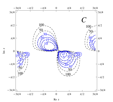
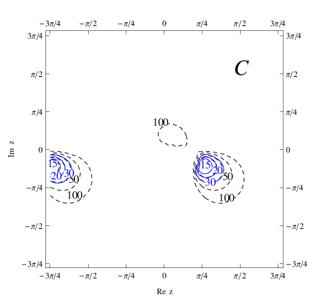
In Fig. 5 we show the contours plots for $M_{1}$ obtained imposing successful leptogenesis, i.e. $\eta=\eta_{B}^{\rm CMB}$ (we used the $2\sigma$ lower value $\eta_{B}^{CMB}=5.9\times 10^{-10}$ ), for $\zeta=+1$ and for initial thermal abundance. The four panels correspond to the four benchmark cases $A$ , $B$ , $C$ and $D$ in the NH case. The solid lines are obtained including the contribution $N_{B-L}^{\rm f(2)}$ in the final asymmetry and therefore represent the main result of the paper. These have to be compared with the dashed lines where this contribution is neglected. In Fig. 5 and indeed in all subsequent figures, one can notice again a periodicity in $\pi$ along ${\rm Re}z$ . This is because final asymmetries are given from eq. (108), for which all terms are dependant upon quantities periodic in $\pi$ along ${\rm Re}z$ (these quantities being the washouts, $p_{12}$ and the CP asymmetries). As one can see, on most of the regions leptogenesis is $N_{1}$ -dominated as one would expect ⁵⁵ 5 The $N_{1}$ -dominated regions are approximately invariant for $z\rightarrow-z$ , implying $N_{B-L}^{\rm f(1,{\cal I})}(z)\simeq N_{B-L}^{\rm f(1,{\cal I})}(-z)$ . This is because $r_{1\alpha}^{\cal I}$ is dominated by the first term in the eq. (94), exactly invariant for $z\rightarrow-z$ , and because the $K_{1\alpha}$ are also approximately invariant for $z\rightarrow-z$ (see upper panels in Fig. 1).. However, there are two regions, around $z\sim\pm\pi/2$ , where the asymmetry is $N_{2}$ -dominated. If $N_{B-L}^{\rm f(2)}$ is neglected, this region would be only partially accessible and in any case only for quite large values $M_{1}\gtrsim 30\times 10^{10}\,{\rm GeV}$ ⁶⁶ 6 Notice that this time there is no invariance with respect to $z\rightarrow-z$ since $r_{2\alpha}^{\cal J}$ is dominated either by the third term (for cases A, B, C,) or by the second term (for case D) in eq. (105) that are not invariant for $z\rightarrow-z$ . On the other hand the second term is invariant for ${\rm Re}\,z\rightarrow-{\rm Re}\,z$ and therefore one could naively expect a specular region at $z\sim-\pi/2$ . However, notice that $K_{2\gamma}$ is not invariant for ${\rm Re}\,z\rightarrow-{\rm Re}\,z$ . In this way, for negative ${\rm Re}\,z$ and same values of $|z|$ , the wash-out is strong and prevents the existence of this specular region..

When the contribution $N_{B-L}^{\rm f(2)}$ is taken into account one can have successful leptogenesis for $M_{1}$ values as low as $1.3\times 10^{11}\,{\rm GeV}$ for benchmark case B and vanishing initial $N_{2}$ -abundance. The existence of these ‘ $N_{2}$ -dominated regions’ is the result of a combination of different effects: i) the value of $(1-p_{12})$ , setting the size of the contribution from $N_{2}$ decays that survives the $N_{1}$ washout, is maximal in these regions as one can see from Fig. 2; ii) the wash-out at the production is in these region minimum as one can see from the plots of $K_{2\tau}$ and $K_{2\gamma}$ (cf. Fig. 1); iii) the $N_{2}$ -flavoured $C\!P$ asymmetries are not suppressed in these regions contrarily to the $N_{1}$ flavoured $C\!P$ asymmetries.

It is interesting to compare the results obtained for the 4 different benchmark cases. A comparison between the case A (upper left panel) and the case $B$ (upper right panel) shows that large values of $\theta_{13}$ and no Dirac phase enhance $N_{B-L}^{\rm f(2)}$ so that the $N_{2}$ -dominated regions get enlarged. On the other hand a comparison between B and C shows that a Dirac phase seems to suppress $N_{B-L}^{\rm f(2)}$ . A comparison between B and D shows that a Majorana phase seems just to change the position of the $N_{2}$ -dominated regions without consistently modify their size differently from the $N_{1}$ -dominated regions that are instead maximised by the presence of non-vanishing Majorana phase as known [30, 13]. Notice that, though this effect is shown only for $\theta_{13}=11.5^{\circ}$ , it actually occurs for any choice of $\theta_{13}$ , in particular for $\theta_{13}=0$ . Interestingly, for non-zero Majorana phase the new region where leptogenesis is favoured now overlaps with the Im $(z)=0$ axis. This means that CP violation for $N_{2}$ -dominated leptogenesis can be successfully induced just by the Majorana phase. We have also checked that varying the low energy parameters within the ranges of values set by the 4 benchmark cases, one has a continuous variation of the allowed regions.

It can be seen that the $N_{2}$ -dominated regions are maximal in case B. For this reason in Fig. 6 we show a zoom of the $N_{2}$ -dominated regions around $z=\pi/2$ for case B. This figure represents one of the main results of this paper.

On the other hand if we consider the IH case, the situation is very different as one can see from Fig. 7. The much stronger wash-out acting both on the $N_{1}$ and on the $N_{2}$ contributions suppresses the final asymmetry in a way that large fraction of the allowed regions disappear, including the $N_{2}$ -dominated regions. The surviving allowed regions are therefore strongly reduced and strictly $N_{1}$ -dominated.

Analogous results are obtained for the branch $\zeta=-1$ , shown in figure 8.

A comparison between the plots obtained for the two branches shows that the the finally asymmetry is invariant for $(\xi,z)\rightarrow(-\xi,-z)$ and this is confirmed by the analytical expressions both for the flavoured decay parameters determining the wash-out and for the $C\!P$ asymmetries.

6 Leptogenesis from two RH neutrinos in models with Light Sequential Dominance

In section 5 (c.f. Figure 6) we have seen that two new favoured region for leptogenesis have appeared where $z\sim\pm\pi/2$ , for $\zeta=\pm 1$ , and for NH. Compared to previous studies where the production of the baryon asymmetry in this region of parameters was thought to be very suppressed, we found that, due to effects from $N_{2}$ decays, leptogenesis is quite efficient and can be realised with comparatively low $M_{1}\sim 10^{11}$ GeV. This result is particularly interesting since $z\sim\pm\pi/2$ corresponds to the class of neutrino mass models with Light Sequential Dominance (LSD) [2], as we will discuss below. The dictionary between the parameter $z$ and the Sequential Dominance (SD) parameters will be given explicitly in section 6.2. Finally, in 6.3 we will discuss the decay asymmetries in an explicit example scenario of LSD and show the enhancement of the asymmetry from $N_{2}$ decays analytically in terms of SD parameters and the deviation from TB mixing.

6.1 Light Sequential Dominance

In models with SD, the RH neutrinos contribute to the neutrino mass matrix with “sequential” strength, leading to a NH. In LSD, the lightest RH neutrino $N_{1}$ provides the largest “dominant” contribution, whereas the second lightest RH neutrino contributes subdominantly. When the heaviest RH neutrino (almost) decouples, we arrive (approximately) at a 2 RH neutrino model.

To understand how SD, and in particular LSD works, we begin by writing the RH neutrino Majorana mass matrix $M_{\mathrm{RR}}$ in a diagonal basis as

M_{\mathrm{RR}}=\left(\begin{array}[]{ccc}M_{1}&0&0\\ 0&M_{2}&0\\ 0&0&M_{3}\end{array}\right),

(116)

where $M_{1}<M_{2}<M_{3}$ . In this basis we write the neutrino (Dirac) Yukawa matrix $\lambda_{\nu}$ in terms of $(1,3)$ column vectors $A_{i},$ $B_{i},$ $C_{i}$ as

Y_{\nu}=\left(\begin{array}[]{ccc}A&B&C\end{array}\right)

(117)

in the convention where the Yukawa matrix is given in left-right convention. Explicitly we have

Y_{\nu}=\left(\begin{array}[]{ccc}A_{1}&B_{1}&C_{1}\\ A_{2}&B_{2}&C_{2}\\ A_{3}&B_{3}&C_{3}\end{array}\right).

(118)

The Dirac neutrino mass matrix is then given by $m_{\mathrm{LR}}^{\nu}=Y_{\nu}\,v_{\mathrm{u}}$ . The term for the light neutrino masses in the effective Lagrangian (after electroweak symmetry breaking), resulting from integrating out the massive RH neutrinos, now reads

\mathcal{L}^{\nu}_{eff}=\frac{(\nu_{i}^{T}A_{i})(A^{T}_{j}\nu_{j})v^{2}}{M_{1}}+\frac{(\nu_{i}^{T}B_{i})(B^{T}_{j}\nu_{j})v^{2}}{M_{2}}+\frac{(\nu_{i}^{T}C_{i})(C^{T}_{j}\nu_{j})v^{2}}{M_{3}}\,,

(119)

where $\nu_{i}$ ( $i=1,2,3$ ) are the left-handed neutrino fields. As stated above, LSD then corresponds to $M_{3}\rightarrow\infty$ so that the third term becomes negligible, with the second term subdominant and the first term dominant [2]:

\frac{A_{i}A_{j}}{M_{1}}\gg\frac{B_{i}B_{j}}{M_{2}}\gg\frac{C_{i}C_{j}}{M_{3}}\,.

(120)

In addition, we shall assume that small $\theta_{13}$ and almost maximal $\theta_{23}$ require that

|A_{1}|\ll|A_{2}|\approx|A_{2}|.

(121)

Constrained Sequential Dominance (CSD) is defined as [37]:

$\displaystyle\|A_{1}\|$	$\displaystyle=$	$\displaystyle 0,$	(122)
$\displaystyle\text{\ }\|A_{2}\|$	$\displaystyle=$	$\displaystyle\|A_{3}\|,$	(123)
$\displaystyle\|B_{1}\|$	$\displaystyle=$	$\displaystyle\|B_{2}\|=\|B_{3}\|,$	(124)
$\displaystyle A^{\dagger}B$	$\displaystyle=$	$\displaystyle 0.$	(125)

CSD implies TB mixing [37] and vanishing leptogenesis if $M_{3}>>M_{1},M_{2}$ [12, 38].

6.2 An $R$ matrix dictionary for LSD

According to LSD, the “dominant” $N_{1}$ , i.e. its mass and Yukawa couplings, governs the largest light neutrino mass $m_{3}$ , whereas the “subdominant” $N_{2}$ governs the lighter neutrino mass $m_{2}$ , while the decoupled $N_{3}$ is associated with $m_{1}\rightarrow 0$ . From eq. (49) it is then clear that, ignoring $m_{2}/m_{3}$ corrections, the R-matrix for LSD takes the approximate form [39]:

R^{LSD}\approx\mathrm{diag}(\pm 1,\pm 1,1)\left(\begin{array}[]{ccc}0&0&1\\ 0&1&0\\ 1&0&0\end{array}\right),

(126)

where the four different combinations of the signs correspond physically to the four different combinations of signs of the Dirac matrix columns associated with the lightest two RH neutrinos of mass $M_{1}$ and $M_{2}$ . The sign of the third column associated with $M_{3}\rightarrow\infty$ is irrelevant and has been dropped since it would in any case just redefine the overall sign of the Dirac mass matrix. These choices of signs are of course irrelevant for the light neutrino phenomenology, since the effect of the orthogonal $R$ matrix cancels in the see-saw mechanism (by definition). The four choices of sign are also irrelevant for type I leptogenesis, since each column enters quadratically in both the asymmetry and the washout formulas in Eqs. (17) and (14), independently of flavour or whether $N_{1}$ or $N_{2}$ is contributing. Comparing eq. (126) to the parameterisation of $R^{(NH)}$ for the 2 RH neutrino models in eq. (53), we see that LSD just corresponds to $z\sim\pm\pi/2$ which correspond to the new regions opened up by $N_{2}$ leptogenesis that were observed numerically in the previous section. To be precise the dictionary for the sign choices in eq. (126) are as follows: for the $\zeta=1$ branch, $z\approx\pi/2$ , corresponds to $\mathrm{diag}(1,-1,1)$ , while $z\approx-\pi/2$ , corresponds to $\mathrm{diag}(-1,1,1)$ ; for the $\zeta=-1$ branch, $z\approx\pi/2$ , corresponds to $\mathrm{diag}(-1,-1,1)$ , while $z\approx-\pi/2$ , corresponds to $\mathrm{diag}(1,1,1)$ . According to the above observation, all four of these regions will contribute identically to leptogenesis, as observed earlier in the numerical and analytical results (i.e. giving identical results for $\zeta=\pm 1$ and $z\approx\pm\pi/2$ ).

We may expand eq. (53) for LSD for any one of these identical regions to leading order in $m_{2}/m_{3}$ . For example consider the case $\zeta=-1$ and $z\approx-\pi/2$ corresponding to the case where all the Dirac columns have the same relative sign, $\mathrm{diag}(1,1,1)$ . Then expanding eq. (53) around $z\approx-\pi/2$ , defining $\Delta\approx z+\frac{\pi}{2}$ , we may write,

R^{LSD}\approx\left(\begin{array}[]{ccc}0&\Delta&1\\ 0&1&-\Delta\\ 1&0&0\end{array}\right).

(127)

Using the results in [40] we find useful analytic expressions which relate the R-matrix angle to the Yukawa matrix elements near the CSD limit of LSD corresponding to small $\Delta$ ,

	$\displaystyle{\rm Re}(\Delta)$	$\displaystyle\approx$	$\displaystyle\frac{{\rm Re}(A^{\dagger}B)v^{2}}{(m_{3}-m_{2})M_{3}^{1/2}M_{2}^{1/2}}$
	$\displaystyle{\rm Im}(\Delta)$	$\displaystyle\approx$	$\displaystyle\frac{{\rm Im}(A^{\dagger}B)v^{2}}{(m_{3}+m_{2})M_{3}^{1/2}M_{2}^{1/2}}\,.$		(128)

Notice that $\Delta\rightarrow 0$ when $A^{\dagger}B\rightarrow 0$ to all orders in $m_{2}/m_{3}$ . This is just the case in CSD due to eq. (125). Thus in the CSD limit of LSD eq. (126) becomes exact [39] to all orders in $m_{2}/m_{3}$ . Clearly, leptogenesis vanishes in CSD which can be understood from the fact that the R-matrix in CSD is real and diagonal (up to a permutation) [38] or from the fact that A is orthogonal to B [12]. However in the next section we consider a perturbation of CSD, allowing leptogenesis but preserving TB mixing.

6.3 Example: perturbing the CSD limit of LSD

Using eq. (17), we obtain, making the usual hierarchical RH neutrino mass assumption the $N_{1}$ contribution to the leptogenesis asymmetry parameter is given by:

\varepsilon_{1\alpha}\approx-\frac{3}{16\pi}\frac{M_{1}}{M_{2}}\frac{1}{A^{\dagger}A}\mathrm{Im}\left[A_{\alpha}^{*}(A^{\dagger}B)B_{\alpha}\right].

(129)

Clearly the asymmetry vanishes in the case of CSD due to eq. (125). In this subsection we consider an example which violates CSD, but maintains TB mixing and stays close to LSD.

Before we turn to an explicit example, let us state the expectation for the size of the decay asymmetries. We expect that, typically,

\varepsilon_{1\mu,\tau}\approx-\frac{3}{16\pi}\frac{m_{2}M_{1}}{v^{2}},\ \ \varepsilon_{1e}\approx\frac{A_{1}}{A_{2}}\varepsilon_{1\mu,\tau}.

(130)

The $N_{2}$ contribution to the leptogenesis asymmetry parameter is given by the interference with the lighter RH neutrino in the loop via the second term in eq. (17), which is indeed often ignored in the literature:

\varepsilon_{2\alpha}\approx-\frac{2}{16\pi}\frac{1}{B^{\dagger}B}\mathrm{Im}\left[B_{\alpha}^{*}(A^{\dagger}B)A_{\alpha}\right].

(131)

This leads to typically,

\varepsilon_{2\mu,\tau}\approx-\frac{1}{16\pi}\frac{m_{3}M_{1}}{v^{2}},\ \ \varepsilon_{2e}\approx\frac{A_{1}}{A_{2}}\varepsilon_{2\mu,\tau}

(132)

which should be compared to eq. (130). The $N_{2}$ contribution to the decay asymmetries looks larger than the $N_{1}$ contribution.

To compare the two asymmetries and the produced baryon asymmetry explicitly, let us now calculate the final asymmetries in a specific perturbation of the Light CSD form. As an example, we may consider

	$\displaystyle(A_{1},A_{2},A_{3})$	$\displaystyle=$	$\displaystyle(0,a,a)$		(133)
	$\displaystyle(B_{1},B_{2},B_{3})$	$\displaystyle=$	$\displaystyle(b,b+q,-b+q)$		(134)

such that

Y_{\nu}=\left(\begin{array}[]{ccc}0&b&C_{1}\\ a&b+q&C_{2}\\ a&-b+q&C_{3}\end{array}\right).

(135)

Providing $|q|\ll|b|$ , this perturbation of CSD but stays close to LSD and allows non-zero leptogenesis. Interestingly this perturbation of CSD also preserves TB mixing as discussed in [40], where more details can be found. Note that $z$ is given by eq. (128) and therefore depends on $a,b$ and $q$ .

For our example, we now obtain (assuming real $a$ and neglecting $q$ in $B^{\dagger}B$ ):

\varepsilon_{1\gamma}\approx-\frac{3}{16\pi}\frac{m_{2}M_{1}}{v^{2}}\frac{\mathrm{Im}[q\,b+q^{2}]}{B^{\dagger}B},\ \ \varepsilon_{1\tau}\approx-\frac{3}{16\pi}\frac{m_{2}M_{1}}{v^{2}}\frac{\mathrm{Im}[-q\,b+q^{2}]}{B^{\dagger}B}.

(136)

The $N_{2}$ contribution to the leptogenesis asymmetry parameter is given by the interference with the lighter RH neutrino in the loop via the second term in eq. (17):

\varepsilon_{2\gamma}\approx-\frac{2}{16\pi}\frac{m_{3}M_{1}}{v^{2}}\frac{\mathrm{Im}[q\,b^{*}]}{B^{\dagger}B},\ \ \varepsilon_{2\tau}\approx-\varepsilon_{2\gamma}

(137)

For the washout parameters, we obtain:

\displaystyle K_{1\gamma}=K_{1\tau}\approx\frac{m_{3}}{m_{*}}

(138)

and

\displaystyle K_{2\gamma}\sim K_{2\tau}\approx\frac{m_{2}}{m_{*}}\>.

(139)

The parameter $p_{12}$ is given by (neglecting $q$ in the last step)

\displaystyle p_{12}\approx-\frac{|A_{1}B_{2}+A_{2}B_{1}|^{2}}{(|A_{1}|^{2}+|A_{2}|^{2})(|B_{1}|^{2}+|B_{2}|^{2})}\approx\frac{1}{2}

(140)

For the final asymmetries from $N_{1}$ decay this means

\displaystyle N_{B-L}^{f(1)}\approx-(\varepsilon_{1\gamma}+\varepsilon_{1\tau})\,\kappa_{1\gamma}\approx 2\frac{3}{16\pi}\frac{m_{2}M_{1}}{v^{2}}\frac{\mathrm{Im}[q^{2}]}{B^{\dagger}B}\kappa(m_{3}/m^{*})

(141)

whereas

\displaystyle N_{B-L}^{f(2)}\approx-(1-p_{12})\varepsilon_{2\gamma}\,\kappa_{2\gamma}\approx\frac{1}{2}\frac{2}{16\pi}\frac{m_{3}M_{1}}{v^{2}}\frac{\mathrm{Im}[q\,b^{*}]}{B^{\dagger}B}\kappa(m_{2}/m^{*})\>.

(142)

So we can estimate:

\displaystyle\frac{N_{B-L}^{f(2)}}{N_{B-L}^{f(1)}}\approx\frac{m_{3}}{m_{2}}\frac{\kappa(m_{2}/m^{*})}{\kappa(m_{3}/m^{*})}\frac{\mathrm{Im}[q\,b^{*}]}{\mathrm{Im}[6\,q^{2}]}.

(143)

We see that, as already anticipated in the beginning of this subsection, there is an enhancement of the asymmetry from the $N_{2}$ decay by a factor of $\frac{m_{3}}{m_{2}}$ (from the decay asymmetries). Furthermore, there is another enhancement factor from the efficiency factor $\kappa$ given by $\frac{\kappa(m_{2}/m^{*})}{\kappa(m_{3}/m^{*})}$ . Both terms imply an enhancement of a factor of 5 each. Finally, the factor $\frac{\mathrm{Im}[q\,b^{*}]}{\mathrm{Im}[6\,q^{2}]}$ can get large for small $q$ , i.e. close to the CSD case. However, of course, closer to the CSD case the decay asymmetries get more and more suppressed.

In summary, in models with Light Sequential Dominance (LSD) the asymmetry from the $N_{2}$ decays is generically larger than the asymmetry from $N_{1}$ decays, in agreement with the results obtained in the previous sections in the R matrix parameterisation. We like to emphasise that in order to calculate the prospects for leptogenesis in models with LSD (in the two flavour regime), it is thus crucial to include the $N_{2}$ decays (which have previously been neglected).

7 Conclusions

We have revisited leptogenesis in the minimal non-supersymmetric type I see-saw mechanism with two hierarchical RH neutrinos ( $M_{2}\gtrsim 3\,M_{1}$ ), including flavour effects and allowing both RH neutrinos $N_{1}$ and $N_{2}$ to contribute, rather than just the lightest RH neutrino $N_{1}$ that has hitherto been considered.

We emphasise two crucial ingredients of our analysis: i) the flavoured $C\!P$ asymmetries have been calculated taking into account also terms that cancel in the total $C\!P$ asymmetries [14] and that have been so far neglected within the two RH neutrino model; ii) Part of the asymmetry produced from $N_{2}$ decays, that one orthogonal in flavour space to the lepton flavour $\ell_{1}$ produced by $N_{1}$ decays, escapes the $N_{1}$ washout [17].

Defining four benchmark points corresponding to a range of PMNS parameters, we have performed scans over the single complex angle $z$ of the orthogonal matrix $R$ for each of the two physically distinct branches $\zeta=\pm 1$ . For the case of a normal mass hierarchy, for each benchmark point we found that in regions around $z\sim\pm\pi/2$ , the $N_{2}$ contribution can dominate the contribution to leptogenesis. For benchmark B corresponding to a large reactor angle and zero low energy CP violation we found that the lightest RH neutrino mass may be decreased by about an order of magnitude in these regions, down to $M_{1}\sim 1.3\times 10^{11}\,{\rm GeV}$ for vanishing initial $N_{2}$ -abundance, with the numerical results supported by analytic estimates. Other benchmarks with smaller reactor angle and/or low energy CP violating phases switched on exhibit similar results.

These $N_{2}$ -dominated regions around $z\sim\pm\pi/2$ are quite interesting since they correspond to light sequential dominance in the hierarchical limit where the atmospheric neutrino mass $m_{3}$ arises dominantly from the lightest RH neutrino of mass $M_{1}$ , the solar neutrino mass $m_{2}$ arises dominantly from the second lightest RH neutrino of mass $M_{2}$ , and the lightest neutrino mass of $m_{1}$ is negligible due to a very large RH neutrino of mass $M_{3}$ . Such a scenario commonly arises in unified models based on a natural application of the see-saw mechanism [12, 41] so the new results in this paper may be relevant to unified model building in large classes of models involving a NH.

Acknowledgments

PDB acknowledges financial support from the NExT Institute and SEPnet. SA acknowledges partial support by the DFG cluster of excellence ‘Origin and Structure of the Universe’. DAJ is thankful to the STFC for providing studentship funding. PDB and SFK were partially supported by the STFC Rolling Grant ST/G000557/1 and SFK was partially supported by the EU ITN grant UNILHC 237920 (‘Unification in the LHC era’).

References

[1] P. Minkowski, Phys. Lett. B 67 (1977) 421; T. Yanagida, in Workshop on Unified Theories, KEK report 79-18 (1979) p. 95; M. Gell-Mann, P. Ramond, R. Slansky, in Supergravity (North Holland, Amsterdam, 1979) eds. P. van Nieuwenhuizen, D. Freedman, p. 315; S.L. Glashow, in 1979 Cargese Summer Institute on Quarks and Leptons (Plenum Press, New York, 1980) p. 687; R. Barbieri, D. V. Nanopoulos, G. Morchio and F. Strocchi, Phys. Lett. B 90 (1980) 91; R. N. Mohapatra and G. Senjanovic, Phys. Rev. Lett. 44 (1980) 912.
[2] S. F. King, Nucl. Phys. B 576 (2000) 85 [arXiv:hep-ph/9912492].
[3] M. Fukugita and T. Yanagida, Phys. Lett. B 174, 45 (1986).
[4] A. Ibarra, JHEP 0601 (2006) 064 [hep-ph/0511136].
[5] P. H. Frampton, S. L. Glashow and T. Yanagida, Phys. Lett. B 548 (2002) 119 [arXiv:hep-ph/0208157].
[6] S. F. King, Phys. Rev. D 67 (2003) 113010 [arXiv:hep-ph/0211228].
[7] P. H. Chankowski and K. Turzynski, Phys. Lett. B 570 (2003) 198 [arXiv:hep-ph/0306059].
[8] A. Ibarra and G. G. Ross, Phys. Lett. B 591 (2004) 285 [arXiv:hep-ph/0312138].
[9] S. Blanchet and P. Di Bari, JCAP 0606 (2006) 023 [arXiv:hep-ph/0603107].
[10] A. Abada, S. Davidson, F. X. Josse-Michaux, M. Losada and A. Riotto, JCAP 0604, 004 (2006); E. Nardi, Y. Nir, E. Roulet and J. Racker, JHEP 0601 (2006) 164.
[11] A. Abada, S. Davidson, A. Ibarra, F. X. Josse-Michaux, M. Losada and A. Riotto, JHEP 0609 (2006) 010 [arXiv:hep-ph/0605281].
[12] S. Antusch, S. F. King and A. Riotto, JCAP 0611 (2006) 011 [arXiv:hep-ph/0609038].
[13] E. Molinaro and S. T. Petcov, Phys. Lett. B 671 (2009) 60 [arXiv:0808.3534 [hep-ph]].
[14] A. Anisimov, S. Blanchet and P. Di Bari, JCAP 0804 (2008) 033 [arXiv:0707.3024 [hep-ph]].
[15] S. Blanchet and P. Di Bari, Nucl. Phys. B 807 (2009) 155 [arXiv:0807.0743 [hep-ph]].
[16] P. Di Bari, Nucl. Phys. B 727 (2005) 318 [arXiv:hep-ph/0502082]; O. Vives, Phys. Rev. D 73 (2006) 073006 [arXiv:hep-ph/0512160]; P. Di Bari and A. Riotto, Phys. Lett. B 671 (2009) 462 [arXiv:0809.2285 [hep-ph]]; P. Di Bari and A. Riotto, JCAP 1104 (2011) 037 [arXiv:1012.2343 [hep-ph]].
[17] R. Barbieri, P. Creminelli, A. Strumia, N. Tetradis, Nucl. Phys. B575 (2000) 61-77. [hep-ph/9911315]; G. Engelhard, Y. Grossman, E. Nardi and Y. Nir, Phys. Rev. Lett. 99 (2007) 081802 [arXiv:hep-ph/0612187].
[18] S. Antusch, P. Di Bari, D. A. Jones and S. F. King, Nucl. Phys. B 856 (2012) 180 [arXiv:1003.5132 [hep-ph]].
[19] E. Komatsu et al., arXiv:1001.4538 [Unknown].
[20] E. W. Kolb, M. S. Turner, The Early Universe, Addison-Wesley, New York, 1990
[21] W. Buchmuller, P. Di Bari and M. Plumacher, Annals Phys. 315 (2005) 305 [arXiv:hep-ph/0401240].
[22] M. Plumacher, Z. Phys. C 74 (1997) 549 [arXiv:hep-ph/9604229].
[23] E. Nezri and J. Orloff, JHEP 0304 (2003) 020 [arXiv:hep-ph/0004227].
[24] L. Covi, E. Roulet and F. Vissani, Phys. Lett. B 384 (1996) 169 [arXiv:hep-ph/9605319].
[25] S. Antusch, S. Blanchet, M. Blennow and E. Fernandez-Martinez, JHEP 1001 (2010) 017 [arXiv:0910.5957 [hep-ph]].
[26] G. F. Giudice, A. Notari, M. Raidal, A. Riotto and A. Strumia, Nucl. Phys. B 685 (2004) 89; C. P. Kiessig, M. Plumacher and M. H. Thoma, Phys. Rev. D 82 (2010) 036007.
[27] S. Blanchet, P. Di Bari and G. G. Raffelt, JCAP 0703 (2007) 012; A. De Simone and A. Riotto, JCAP 0702 (2007) 005; M. Beneke, B. Garbrecht, C. Fidler, M. Herranen and P. Schwaller, Nucl. Phys. B 843 (2011) 177.
[28] A. De Simone and A. Riotto, JCAP 0708 (2007) 002; M. Beneke, B. Garbrecht, M. Herranen and P. Schwaller, Nucl. Phys. B 838 (2010) 1; A. Anisimov, W. Buchmuller, M. Drewes and S. Mendizabal, arXiv:1012.5821.
[29] A. Basboll and S. Hannestad, JCAP 0701 (2007) 003; F. Hahn-Woernle, M. Plumacher and Y. Y. Y. Wong, JCAP 0908 (2009) 028.
[30] S. Blanchet and P. Di Bari, JCAP 0703 (2007) 018.
[31] J. A. Casas and A. Ibarra, Nucl. Phys. B 618, 171 (2001) [arXiv:hep-ph/0103065].
[32] M. C. Gonzalez-Garcia and M. Maltoni, Phys. Rept. 460 (2008) 1; T. Schwetz, M. Tortola and J. W. F. Valle, arXiv:0808.2016 [hep-ph].
[33] C. Amsler et al. [Particle Data Group], Phys. Lett. B 667, 1 (2008).
[34] P. F. Harrison, D. H. Perkins and W. G. Scott, Phys. Lett. B 530 (2002) 167 [arXiv:hep-ph/0202074].
[35] et al. [T2K Collaboration], arXiv:1106.2822 [Unknown].
[36] S. Davidson and A. Ibarra, Phys. Lett. B 535, 25 (2002).
[37] S. F. King, JHEP 0508 (2005) 105 [arXiv:hep-ph/0506297].
[38] S. Choubey, S. F. King and M. Mitra, Phys. Rev. D 82 (2010) 033002 [arXiv:1004.3756 [hep-ph]].
[39] S. F. King, Nucl. Phys. B 786 (2007) 52 [arXiv:hep-ph/0610239].
[40] S. F. King, JHEP 1101 (2011) 115 [arXiv:1011.6167 [hep-ph]].
[41] S. Antusch and S. F. King, New J. Phys. 6 (2004) 110 [arXiv:hep-ph/0405272]; S. Antusch, S. F. King, C. Luhn and M. Spinrath, Nucl. Phys. B 850 (2011) 477 [arXiv:1103.5930 [hep-ph]]; S. Antusch, S. F. King and M. Spinrath, Phys. Rev. D 83 (2011) 013005 [arXiv:1005.0708 [hep-ph]].

Leptogenesis in the two right-handed neutrino model revisited

Abstract

1 Introduction

2 General Set up and notation

3 An analytical solution for the final asymmetry from Boltzmann equations

3.1 Production of the asymmetry from N2N_{2} processes

3.2 Production and wash-out of the asymmetry from N1N_{1} processes

4 Combining the low energy neutrino data with the orthogonal parametrization

4.1 Orthogonal parametrization for the two RH neutrino model

4.2 Decay parameters in the orthogonal parametrization

4.3 CP Asymmetries in the orthogonal parametrization

4.3.1 Lightest RH neutrino C​PC\!P asymmetries

4.3.2 Next-to-lightest RH neutrino

5 Constraints on the parameter space and N1N_{1} versus N2N_{2} contribution

6 Leptogenesis from two RH neutrinos in models with Light Sequential Dominance

6.1 Light Sequential Dominance

6.2 An RR matrix dictionary for LSD

6.3 Example: perturbing the CSD limit of LSD

7 Conclusions

Acknowledgments

References

3.1 Production of the asymmetry from $N_{2}$ processes

3.2 Production and wash-out of the asymmetry from $N_{1}$ processes

4.3.1 Lightest RH neutrino $C\!P$ asymmetries

5 Constraints on the parameter space and $N_{1}$ versus $N_{2}$ contribution

6.2 An $R$ matrix dictionary for LSD