Measurement of the cosmic-ray antiproton spectrum at solar minimum with a long-duration balloon flight over Antarctica
Abstract
The energy spectrum of cosmic-ray antiprotons (’s) from 0.17 to 3.5 GeV has been measured using 7886 ’s detected by BESS-Polar II during a long-duration flight over Antarctica near solar minimum in December 2007 and January 2008. This shows good consistency with secondary calculations. Cosmologically primary ’s have been investigated by comparing measured and calculated spectra. BESS-Polar II data show no evidence of primary ’s from evaporation of primordial black holes.
pacs
Valid PACS appear herePrecise measurement of the cosmic-ray antiproton () spectrum is crucial to investigations of conditions in the early universe and cosmic-ray propagation. Most cosmic-ray ’s are produced by interactions of cosmic-ray nuclei with the interstellar gas. The energy spectrum of these “secondary” ’s peaks near 2 GeV, decreasing sharply below and above due to the kinematics of production and to the local interstellar (LIS) proton spectrum. The secondary ’s offer a unique probe [1, 2, 3] of cosmic-ray propagation and solar modulation. Cosmologically “primary” sources have also been suggested, including the annihilation of dark-matter particles and the evaporation of primordial black holes (PBH) by Hawking radiation [4].
Small PBHs, formed in the early Universe by initial density fluctuations, phase transitions, or the collapse of cosmic strings, might have a significant evaporation rate at the current age of the Universe and could contribute to the measured spectrum at low energies [5]. Because the predicted LIS PBH spectrum peaks at MeV, this would be strongly influenced by solar modulation, so a search is most sensitive at solar minimum [6].
BESS95+97 showed that the spectrum peaks around 2 GeV [7], and measurements by BESS and other experiments have shown that ’s are predominantly secondary [8]. However, the low-energy spectrum measured by BESS95+97 at the previous solar minimum was slightly flatter than predicted by secondary models. Although this suggested the possible presence of primary ’s, the large statistical error of the BESS95+97 data did not allow a firm conclusion. BESS-Polar [9, 8, 10, 11, 12, 13] was developed to evaluate the possibility of excess low-energy flux, with unprecedented precision, using long-duration solar-minimum flights over Antarctica. BESS-Polar I flew in December 2004 [14, 15, 16, 17] and BESS-Polar II [15] flew near solar minimum in December 2007 and January 2008. Here, we report measurements of cosmic-ray ’s from 0.17 GeV to 3.5 GeV by BESS-Polar II and discuss the implications for secondary models and possible primary sources.
|
|
|
|
|
|
|
| ||||||||||||||||||
|---|---|---|---|---|---|---|---|---|---|---|---|---|---|---|---|---|---|---|---|---|---|---|---|---|---|
| 0.17–0.23 | 0.20 | 29 | 0.0 | 3.56 | 0.98–1.07 | 1.03 | 238 | 0.1 | 1.75 | ||||||||||||||||
| 0.23–0.27 | 0.25 | 26 | 0.0 | 4.53 | 1.07–1.17 | 1.12 | 283 | 0.2 | 1.91 | ||||||||||||||||
| 0.27–0.32 | 0.30 | 38 | 0.0 | 5.09 | 1.17–1.28 | 1.23 | 304 | 0.6 | 1.82 | ||||||||||||||||
| 0.32–0.37 | 0.35 | 69 | 0.0 | 7.55 | 1.28–1.40 | 1.34 | 399 | 1.7 | 2.28 | ||||||||||||||||
| 0.37–0.41 | 0.39 | 44 | 0.0 | 8.05 | 1.40–1.53 | 1.47 | 412 | 3.5 | 2.07 | ||||||||||||||||
| 0.41–0.44 | 0.42 | 56 | 0.0 | 9.19 | 1.53–1.68 | 1.60 | 466 | 6.2 | 2.10 | ||||||||||||||||
| 0.44–0.48 | 0.46 | 68 | 0.0 | 9.95 | 1.68–1.84 | 1.75 | 485 | 9.0 | 1.91 | ||||||||||||||||
| 0.48–0.53 | 0.50 | 87 | 0.0 | 1.14 | 1.84–2.01 | 1.92 | 555 | 11.5 | 2.05 | ||||||||||||||||
| 0.53–0.57 | 0.55 | 84 | 0.0 | 9.30 | 2.01–2.20 | 2.11 | 632 | 12.9 | 2.18 | ||||||||||||||||
| 0.57–0.63 | 0.60 | 122 | 0.0 | 1.26 | 2.20–2.41 | 2.31 | 622 | 13.7 | 1.88 | ||||||||||||||||
| 0.63–0.68 | 0.65 | 131 | 0.0 | 1.20 | 2.41–2.64 | 2.53 | 678 | 13.8 | 1.95 | ||||||||||||||||
| 0.68–0.75 | 0.71 | 154 | 0.0 | 1.32 | 2.64–2.89 | 2.76 | 637 | 13.3 | 1.77 | ||||||||||||||||
| 0.75–0.82 | 0.78 | 157 | 0.0 | 1.30 | 2.89–3.16 | 3.00 | 494 | 12.5 | 1.90 | ||||||||||||||||
| 0.82–0.89 | 0.86 | 209 | 0.0 | 1.84 | 3.16–3.46 | 3.28 | 213 | 11.5 | 1.64 | ||||||||||||||||
| 0.89–0.98 | 0.94 | 194 | 0.0 | 1.51 | |||||||||||||||||||||
BESS-Polar is a high-resolution magnetic-rigidity spectrometer. A uniform field of 0.8 T is produced in a thin superconducting solenoid filled with drift-chamber tracking detectors. Particle trajectories are determined by fitting up to 52 hit points with a resolution of m in the bending plane, giving a magnetic-rigidity () resolution of at 1 GV and an overall maximum detectable rigidity (MDR) of 240 GV. Upper (UTOF) and lower (LTOF) scintillator hodoscopes measure time-of-flight (TOF) and d/d and provide the event trigger. For BESS-Polar II measurements, the acceptance is 0.23 m2sr. TOF resolution between the UTOF and LTOF is 120 ps, giving a resolution of 2.5%. A threshold-type Cherenkov counter (ACC), using a silica aerogel radiator with optical index , rejects and backgrounds by a factor of 6100 to identify ’s up to 3.5 GeV [18]. A thin scintillator middle-TOF (MTOF) on the lower surface of the solenoid bore detects low-energy particles that cannot penetrate the magnet wall. TOF resolution between the UTOF and MTOF is 320 ps. In the present analysis, the MTOF was used to independently verify the procedure for eliminating interacting upward-going protons that could mimic low-energy ’s.

BESS-Polar II was launched on December 23, 2007, from Williams Field, near the US McMurdo Station in Antarctica, observing for 24.5 days with the magnet energized. The float altitude was 34 km to 38 km (residual air of 5.8 g/cm2 on average), and the cutoff rigidity was below 0.5 GV. events were acquired with no inflight event selection as 13.6 terabytes of data.
In flight, most detectors and instrument systems operated well, with expected performance. Although the central tracker exhibited high-voltage fluctuations, normal resolution was preserved for more than 90% of the observation time by using algorithms that calibrate the tracker over short time intervals and depend on its high-voltage state. Two TOF PMTs with high-voltage control problems were turned off, one on a UTOF paddle (of 10) and one on an LTOF paddle (of 12). Requiring two good PMTs on each paddle reduced acceptance .
Analysis was performed as described in Ref. [17]. The same selection criteria were applied for ’s and protons because they behave similarly in the symmetric configuration of BESS-Polar, except for deflection direction.
Figure 1 shows versus rigidity plots for events surviving d/d and ACC cuts. A clean, narrow band of 7886 ’s mirrors the protons. The calculated and background is 0.0%, 1.0%, and 2.3% in the 0.2–1.0 GeV, 1.0–2.0 GeV, and 2.0–3.5 GeV energy bands. Other backgrounds, such as albedo, mismeasured positive-rigidity particles, and re-entrant albedo, were negligible.
The differential flux of ’s at the top of atmosphere () integrated over d can be expressed as:
| (1) | |||
| (2) |
where is live time, and and are numbers of observed candidates and expected background particles. For the present analysis 1286460 seconds. The effective geometric acceptance, including noninteraction efficiency , was calculated using GEANT3 as 0.133 0.011 m2sr at 0.2 GeV and 0.159 0.008 m2sr at 2.0 GeV, with errors estimated from differences relative to GEANT4. The detection efficiency for ’s () was calculated using a noninteracting proton sample as 81.4 0.1 % at 0.2 GeV and 60.0 0.2 % at 2.0 GeV. To obtain , corrections were applied for survival probability [19] in the residual atmosphere () and estimated atmospheric production (). was estimated as 85.6 2.0 % at 0.2 GeV and 89.8 2.0 % at 2.0 GeV. , 17.6 3.2 % of the detected ’s at 0.2 GeV and 27.6 5.0 % at 2.0 GeV, was calculated by solving simultaneous transport equations [19] with adjusted interaction length () and tertiary production [20]. The uncertainty in this calculation is 18.1% .
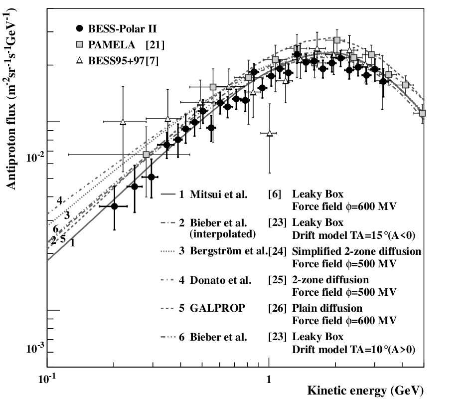
Table 1 gives the flux of ’s at TOA from 0.17 to 3.5 GeV with the statistical (first) and systematic (second) errors. The dominant systematics are atmospheric subtraction and detection efficiency. A rapid change in efficiency due to the ACC veto increases the systematic uncertainty in the two highest bins.
Fig. 2 shows the BESS-Polar II spectrum with BESS95+97 and PAMELA [21] measurements and solar-minimum secondary calculations [6, 22, 23, 24, 25, 26]. Curve 1 uses Mitsui et al. [6, 22] data with force-field modulation of 600 MV from the best fit to the BESS-Polar II proton spectrum. Curve 2 was generated by interpolating model calculations supplied by Bieber et al. [23] for negative solar magnetic field polarity (A0). The tilt angle of 15∘(A0) is the best fit to the BESS-Polar II proton data. Curve 6 is the published A0 solar-minimum calculation [23] for comparison to the BESS95+97 measurements. Curves 3 [24] and 4 [25] are also published solar-minimum calculations. Curve 5 was generated using the GALPROP model [26] with 600 MV force-field modulation. Improved statistical precision of the measured flux results from 14 and 30 times more events below 1 GeV than BESS95+97 and PAMELA, respectively. The BESS-Polar II and PAMELA spectra generally agree in shape, but differ in absolute flux. The weighted mean difference, with combined uncertainties, is 14 5%, calculated near 2 GeV to reduce modulation effects. Both are consistent with solar-minimum secondary calculations. Neither exhibits the flattening at low energies found by BESS95+97, although the differences are statistically small.

The evident differences among the calculations shown in Fig. 2 arise from several factors that can affect the normalization or shape of the spectrum: (1) definition of the primary proton and helium spectra, (2) incomplete knowledge of nuclear physics in propagation, (3) parameters and models of propagation in the Galaxy, and (4) modulation in the heliosphere. Variation in the absolute fluxes of interstellar protons and helium, for instance, affects the absolute flux of ’s, but not the spectral shape.
Precise measurement of the low-energy spectrum by BESS-Polar II allows secondary flux calculations to be evaluated by comparing observed and predicted spectral shapes, as shown in Fig. 3. The calculations are normalized to BESS-Polar II at 2 GeV to focus on their shapes. The calculated spectra and data points are also multiplied by to emphasize differences at low energies. The observed data are not normalized. Chi-square () calculated with BESS-Polar II data and the normalized secondary calculations in Fig. 3 are 0.61 (1), 0.61 (2), 1.32 (3), 1.70 (4), 0.67 (5). The shape variation from uncertainty in the level of solar modulation is illustrated by the lower shaded band, calculated with the Mitsui et al. model [6, 22] and modulation parameters of 500 MV (=0.81) and 700 MV (=0.52). The small sensitivity of drift calculations to tilt angle is shown by the upper shaded band using A0 Bieber et al. data [23] at 10∘ and 20∘ (interpolated). In both cases, the change in spectral shape is small compared to differences arising from propagation models, because of the peaked shape of the LIS secondary spectrum. BESS-Polar II results are more consistent with models (curves 1, 2, and 5) without low-energy ’s from tertiary interactions (curve 3) or a soft spectrum from diffusive reacceleration (curve 4).

The likelihood of primary ’s from PBH evaporation can be quantified by a model-dependent evaporation rate () determined by fitting a PBH model spectrum to the difference of a secondary calculation from the measured flux. is positive (physical) only if the measured flux exceeds the secondary prediction. To avoid bias from uncertainties in the predicted absolute flux, the secondary calculation is normalized to the measurements at the spectral peak (2 GeV) as in Fig. 3. Comparing the models shown in Fig. 3 to the measurements, only 1 and 5 give a significant, and almost identical, excess. We use curve 1, a slightly better fit to the measured spectrum, to calculate . Using the Maki et al. PBH model [5] with force-field modulation gives , as shown in Fig. 4. This excludes by more than 9 sigma the slight possibility of primary ’s suggested by from BESS95+97 data with the same models and modulation. We also find a 90% confidence level upper limit of . This is almost insensitive to modulation (500 MV: , 600 MV: , 700 MV: ).
The affects of charge-sign dependent modulation in the A0 and A0 solar magnetic field polarities on secondary and possible PBH primary fluxes differ considerably because of their spectral shapes. Curves 2 and 6 in Fig. 2 indicate that the differences in the solar-minimum secondary fluxes are small. However, the predicted LIS PBH spectrum peaks near the lower end of the BESS-Polar II energy range, and solar polarity would strongly affect the contribution of primaries to the measured low-energy flux. The primary flux should be suppressed for A0 and higher for A0. Thus, solar polarity cannot explain the excess reported by BESS95+97 or the negligible excess in the BESS-Polar II results reported here. Within statistics, the BESS-Polar II data show no evidence of primary ’s from PBH evaporation.
The BESS-Polar collaboration is supported in Japan by the Grant-in-Aid ‘KAKENHI’ for Specially Promoted and Basic Researches, MEXT-JSPS, and in the U.S. by NASA. Balloon flight operations were carried out by the NASA Columbia Scientific Balloon Facility and the National Science Foundation United States Antarctic Program. We would like to express our sincere thanks for their continuous professional support.
References
- [1] T. K. Gaisser and R. K. Schaefer, Astrophys. J. 394, 174 (1992).
- [2] K. Yoshimura, Adv. Space Res. 27, 693 (2001).
- [3] A. W. Strong, I. V. Moskalenko, and O. Reimer, Astrophys. J. 613, 962 (2004).
- [4] S. W. Hawking, Commun. Math. Phys. 43, 199 (1975).
- [5] K. Maki, T. Mitsui, and S. Orito, Phys. Rev. Lett. 76, 3474 (1996).
- [6] T. Mitsui, K. Maki, and S. Orito, Phys. Lett. B389, 169 (1996).
- [7] S. Orito et al., Phys. Rev. Lett. 84, 1078 (2000).
- [8] J. W. Mitchell et al., Nucl. Phys. (Proc. Suppl.) 134, 31 (2004).
- [9] A. Yamamoto et al., Adv. Space Res. 30, 1253 (2002).
- [10] T. Yoshida et al., Adv. Space Res. 33, 1755 (2004).
- [11] Y. Ajima et al., Nucl. Instrum. Meth. A443, 71 (2000).
- [12] S. Haino et al., Nucl. Instrum. Meth. A518, 167 (2004).
- [13] S. Haino et al., Phys. Lett. B594, 35 (2004).
- [14] A. Yamamoto et al., Adv. Space Res. 42, 442 (2008).
- [15] K. Yoshimura et al., Adv. Space Res. 42, 1664 (2008).
- [16] M. Sasaki et al., Adv. Space Res. 42, 450 (2008).
- [17] K. Abe et al., Phys. Lett. B670, 103 (2008).
- [18] Y. Asaoka et al., Nucl. Instrum. Meth. A416, 236 (1998).
- [19] S. A. Stephens, Astropart. Phys. 6, 229 (1999).
- [20] K. Yamato et al., Phys. Lett. B632, 475 (2006).
- [21] O. Adriani et al., Phys. Rev. Lett. 105, 121101 (2010).
- [22] T. Mitsui, Ph.D. thesis, University of Tokyo (1996).
- [23] J. W. Bieber et al., Phys. Rev. Lett. 83, 674 (1999); J. W. Bieber, private communication (2001).
- [24] L. Bergström, J. Edsjo, and P. Ullio, Astrophys. J. 526, 215 (1999).
- [25] F. Donato et al., Astrophys. J. 563, 172 (2001).
- [26] A. W. Strong and I. V. Moskalenko, Astrophys. J. 509, 212 (1998).