Nuclear energy density functional from
chiral two- and three-nucleon
interactions11
1
Work supported in part by BMBF, GSI and the DFG
cluster of excellence: Origin and Structure of the Universe.
J.W. Holt, N. Kaiser and W. Weise
Physik Department, Technische Universität München,
D-85747 Garching, Germany
email: nkaiser@ph.tum.de
PACS: 12.38.Bx, 21.30.Fe, 21.60.-n, 31.15.Ew
Keywords: Nuclear energy density functional; Density-matrix expansion;
Chiral two- and three-nucleon interactions
Abstract
An improved density-matrix expansion is used to calculate the nuclear energy density functional from chiral two- and three-nucleon interactions. The two-body interaction comprises long-range one- and two-pion exchange contributions and a set of contact terms contributing up to fourth power in momenta. In addition we employ the leading order chiral three-nucleon interaction with its parameters and fixed in calculations of nuclear few-body systems. With this input the nuclear energy density functional is derived to first order in the two- and three-nucleon interaction. We find that the strength functions and of the surface and spin-orbit terms compare in the relevant density range reasonably with results of phenomenological Skyrme forces. However, an improved description requires (at least) the treatment of the two-body interaction to second order. This observation is in line with the deficiencies in the nuclear matter equation of state that remain in the Hartree-Fock approximation with low-momentum two- and three-nucleon interactions.
1 Introduction
The nuclear energy density functional approach is the many-body method of choice in order to calculate the properties of medium-mass and heavy nuclei in a systematic manner [1, 2]. Parameterized non-relativistic Skyrme functionals [3, 4] as well as relativistic mean-field models [5, 6] have been widely and successfully used for such nuclear structure calculations. A complementary approach [7, 8, 9, 10] focuses less on the fitting of experimental data, but attempts to constrain the analytical form of the functional and the values of its couplings from many-body perturbation theory and the underlying two- and three-nucleon interaction. Switching from conventional hard-core NN-potentials to low-momentum interactions [11, 12] is essential in this respect, because the nuclear many-body problem formulated in terms of the latter becomes significantly more perturbative. Indeed, second-order perturbative calculations including also three-body forces give already a good account of the bulk correlations in infinite nuclear matter [13, 14] and in doubly-magic nuclei [15].
In many-body perturbation theory the contributions to the energy are written in terms of density-matrices convoluted with the finite-range interaction kernels, and are therefore highly non-local in both space and time. In order to make such functionals numerically tractable in heavy open-shell nuclei it is desirable to develop simplified approximations for these functionals in terms of local densities and currents only. In such a construction the density-matrix expansion comes prominently into play as it removes the non-local character of the exchange (Fock) contribution to the energy by mapping it onto a generalized Skyrme functional with density-dependent couplings. For some time the prototype for that has been the density-matrix expansion of Negele and Vautherin [16], but recently Gebremariam, Duguet and Bogner [17] have developed an improved version for spin-unsaturated nuclei. They have demonstrated that phase-space averaging techniques allow for a consistent expansion of both the spin-independent (scalar) part as well as the spin-dependent (vector) part of the density-matrix. The improved properties of the new phase-space averaged density-matrix expansion have been extensively studied via the Fock energy densities arising from schematic finite-range central, tensor and spin-orbit interactions for a large set of semi-magic nuclei (for further details see ref.[17]).
In order to match with these new developments, the nuclear energy density functional as it emerges from chiral pion-nucleon dynamics has been recalculated in ref.[18]. This calculation has treated for isospin-symmetric (i.e. ) nuclear systems the effects from -exchange, iterated -exchange, and irreducible -exchange with intermediate -isobar excitations, including Pauli-blocking corrections up to three-loop order. Among other things, it has been found that the two- and three-body contributions to the spin-orbit coupling strength , as generated by -exchange, tend to cancel each other in the relevant density range fm-3, thus leaving room for the short-range nuclear spin-orbit interaction. The short-range components of the NN-interaction together with the constraints on them provided by the elastic scattering data (i.e. NN-phase shifts etc.) have not been considered explicitly in ref.[18]. Furthermore, a similar calculation of a microscopically constrained nuclear energy density functional derived from the chiral NN-potential at next-to-next-to-leading order (N2LO) has been presented recently by Gebremariam, Bogner and Duguet in ref.[19]. They have proposed that the density-dependent couplings associated with the pion-exchange interactions should be added to a standard Skyrme functional (with several adjustable parameters). In the sequel it has been demonstrated in ref.[20] that this new energy density functional gives numerically stable results and that it exhibits a small but systematic reduction of the -measure compared to standard Skyrme functionals (without any pion-exchange terms).
The purpose of the present paper is to derive a nuclear energy density functional with improved (chiral) two- and three-nucleon interactions. We use for the two-body interaction the N3LO chiral NN-potential which reaches at this order the quality of a high-precision NN-potential (in reproducing empirical NN-shifts and deuteron properties). The N3LO chiral potential consists of long-range one- and two-pion exchange terms and two dozen low-energy constants which parameterize the short-distance part of the NN-interaction. The latter contact potential written in momentum space gives the most general contribution up to fourth power in momenta. In the actual calculation we will use the version N3LOW of the chiral NN-potential developed in refs.[21, 22] by lowering the cut-off scale to MeV. This value coincides with the resolution scale inherent to the universal low-momentum NN-potential [11, 12] to which all realistic NN-potentials flow after integrating out effects from momenta above the cut-off scale fm-1. The low-momentum two-body interaction N3LOW is supplemented by the leading order chiral three-nucleon interaction with its parameters , and determined in calculations of nuclear few-body systems [13, 23]. Our paper is organized as follows. In section 2 we recall the basic features of the (improved) density-matrix expansion and the nuclear energy density functional for isospin-symmetric systems. In section 3 we present the two-body contributions to the various density-dependent strength functions , , , and , separately for the finite-range pion-exchange and the zero-range contact interactions. In section 4, we collect the corresponding analytical expressions for the three-body contributions grouped into contact (), -exchange () and -exchange () terms. Section 5 is devoted to the discussion of our numerical results and sections 6 ends with a summary and an outlook.
2 Density-matrix expansion and energy density functional
The starting point for the construction of an explicit nuclear energy density functional is the density-matrix as given by a sum over the energy eigenfunctions representing occupied orbitals of the (non-relativistic) many-fermion system. According to Gebremariam, Duguet and Bogner [17] it can be expanded in relative and center-of-mass coordinates, and , as follows:
| (1) | |||||
with the spherical Bessel function . The quantities appearing on the right hand side of eq.(1) are: the (local) nucleon density , the (local) kinetic energy density and the (local) spin-orbit density . As shown in section 2 of ref.[18] the Fourier transform of the expanded density-matrix eq.(1) with respect to both coordinates and defines in momentum space a ”medium insertion”:
| (2) | |||||
for inhomogeneous many-nucleon systems characterized by the time-reversal-even fields , and . Note that the delta-function in eq.(2) gives weight to the momentum-dependent NN-interactions only in the vicinity of the local Fermi momentum, .
Up to second order in spatial gradients (i.e. deviations from homogeneity) the energy density functional relevant for even-even nuclei reads:
| (3) | |||||
Here, is the energy per particle of isospin-symmetric nuclear matter evaluated at the local nucleon density . The strength function introduces an effective (density-dependent) nucleon mass and it is related to the single-particle potential as follows:
| (4) |
with . The second equality establishes the equivalent relation to the spin and isospin independent p-wave Landau parameter . The strength function of the surface term has the decomposition [18]:
| (5) |
where comprises all those contributions for which the -factor originated directly from the momentum dependence of the interactions in an expansion up to order . Note that only the (fixed) nuclear matter piece of the density-matrix expansion goes into the derivation of the strength function . The second to last term in eq.(3) is responsible for the spin-orbit interaction in nuclei. The associated function measures therefore the strength of the nuclear spin-orbit coupling.
3 Two-body contributions
In this section we work out the two-body contributions to the various density-dependent strength functions which build up the nuclear energy density functional written in eq.(3). Ideally, one would like to use for this task the universal low-momentum NN-potential [12]. However, it is generally given in terms of (off-shell) partial wave matrix elements which makes its application to the density-matrix expansion rather cumbersome. An explicit representation of the momentum space NN-potential in terms of spin- and isospin-operators is much better suited for this purpose. For this reason we use (as a substitute for ) the chiral NN-potential N3LOW developed in refs.[21, 22] by lowering the cut-off scale to MeV. This value of coincides with the resolution scale inherent to the universal low-momentum NN-potential . The finite-range part of the N3LOW chiral NN-potential consists of one- and two-pion exchange pieces which can be summarized in the form:22 2 Note that we associate here the tensor interaction with the operator . This operator splits as into the genuine tensor operator and a spin-spin piece.
| (6) | |||||
where denotes the momentum transfer and the center-of-mass momentum. As usual, and are the spin- and isospin operators of the two nucleons. A special and simplifying feature of is that all the occurring potentials depend only on the momentum transfer and that a quadratic spin-orbit component is absent. The relativistic -correction to the -exchange [24] which does (partially) not share this property is so small that it can be safely neglected. In order to specify our sign and normalization convention, we give also the explicit expression for the -exchange, , with the parameters , MeV and MeV.


The solid and dashed lines in Figs. 1,2,3,4 show the finite-range isoscalar and isovector potentials extracted from the chiral NN-interaction N3LOW [22] in the central, spin-spin, tensor, and spin-orbit channel, respectively. In each figure the curves extend up to momentum transfers of MeV, corresponding to the region within which the interaction gets probed for nuclear densities up to fm-3. One notices in Fig. 3 the large negative values of (multiplied with in ) which result at small momentum transfers from -exchange.
In the (first-order) Hartree-Fock approximation the finite-range NN-potential leads in combination with the density matrix-expansion (i.e. by employing the product of two medium insertions ), to the following two-body contributions to the energy density functional :
| (7) | |||||
| (8) |
| (9) |
| (10) |
| (11) |
setting . The double-prime in eq.(9) denotes a second derivative and we have given the numerical value for resulting from the negative curvature of isoscalar central potential shown in Fig. 1. One can easily convince oneself that as given in eq.(11) stays finite in the limit . After expanding the integrand to linear order in , the constant integrates to zero.
In addition to the finite-range pieces written in eqs.(7-11) there are the two-body contributions from the zero-range contact potential of the chiral NN-interaction N3LOW. The corresponding expression in momentum space includes constant, quadratic, and quartic terms in momenta and it can be found in section 2.2 of ref.[25]. The Hartree-Fock contributions from the NN-contact potential to the nuclear energy density functional read:
| (12) |
| (13) |
| (14) |
| (15) |
| (16) |
The 24 low-energy constants , and are determined (at the cut-off scale of MeV) in fits to empirical NN-phase shifts and deuteron properties [22]. We have extracted their values from the pertinent NN-scattering code made available to us by R. Machleidt. The values of the low-energy constants for the pure contact terms are: , (in units GeV-2), those of the terms quadratic in momenta are: , , , , , , (in units GeV-4), and those of the terms quartic in momenta are: , , , , , , , , , , , , , , (in units GeV-6). Let us mention that the contributions proportional to and in eqs.(12-16) have also been worked out in appendix B of ref.[19] and we find agreement with their results. The terms proportional to as well as the master formulas eqs.(7-11) for the finite-range contributions are new. Note that we do not include an additional regulator function [22] since the NN-interactions are probed only at small momenta MeV.
4 Three-body contributions
In this section we work out the three-body contributions to the nuclear energy density functional . We employ the leading order chiral three-nucleon interaction [23] which consists of a contact piece (with parameter ), a -exchange component (with parameter ) and a -exchange component (with parameters , and ). In order to treat the three-body correlations in inhomogeneous nuclear many-body systems we follow ref.[18] and assume that the relevant product of density-matrices can be represented in momentum space in a factorized form by . Such a factorization ansatz respects by construction the correct nuclear matter limit, but it involves approximations in comparison to more sophisticated treatments outlined in section 4 of ref.[9]. Actually, our approach is similar to the method DME-I introduced in ref.[9].

4.1 -term
We start with the three-body contributions from the contact interaction as represented by the left diagram in Fig. 5. With three (inhomogeneous) medium insertions one finds the following contribution to the energy per particle:
| (17) |
which is quadratic in the density . Obviously, the contributions to the other strength functions vanish due to the momentum-independence of the contact interaction. For the choice of scale MeV the value has been determined in calculations of few-nucleon systems [13] (employing in addition for the two-body interaction).
4.2 -term
Next, we consider the three-body contributions from the -exchange component of the chiral 3N-interaction as represented by the right diagram in Fig. 5. Putting in three (inhomogeneous) medium insertions one finds the following analytical expressions:
| (18) |
| (19) |
| (20) |
| (21) |
with the abbreviation . For the parameter we take the value from ref.[13]. Note that there is no contribution to the spin-orbit coupling strength .
4.3 Hartree diagram proportional to
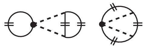
We continue with the three-body contributions from the -exchange Hartree diagram shown in the left part of Fig. 6. Again with three (inhomogeneous) medium insertions one derives the following analytical results:
| (22) | |||||
| (23) | |||||
| (24) | |||||
| (25) |
| (26) |
which depend only on the two isoscalar coupling constants and with values GeV-1 and GeV-1 [23]. Note that the expression for in eq.(25) gives the dominant part of the three-body spin-orbit coupling strength suggested originally by Fujita and Miyazawa [26]. Their proposed mechanism is based on the excitation of a -resonance. In the present approach the two-step process is replaced by an equivalent contact vertex proportional to .
4.4 Fock diagram proportional to
Finally, there are the three-body contributions from the -exchange Fock diagram shown in the right part of Fig. 6. With one single closed nucleon ring this diagram generates (for isospin-symmetric nuclear matter) also non-vanishing contributions from the isovector contact vertex proportional to . We take consistently the value GeV-1 used in few-body calculations by ref.[23]. In the case of the three-body Fock diagram not all of the occurring integrals over the three Fermi spheres can be solved analytically. Collecting all the emerging pieces, we find the following results for the Fock contributions to the nuclear energy density functional :
| (27) | |||||
| (28) | |||||
| (29) | |||||
| (30) | |||||
| (31) | |||||
Here we have introduced the auxiliary functions:
| (32) | |||||
| (33) | |||||
| (34) |
where . A good check of all formulas collected in this section is provided by their Taylor expansion in . Despite the superficial first appearance to the contrary, one can verify that the leading term in the -expansion is . In several cases it is even a higher power of .
5 Results and discussion

In this section we present and discuss our numerical results obtained by summing the series of two- and three-body contributions given in sections 3 and 4. The physical input parameters are: (nucleon axial vector coupling constant), MeV (pion decay constant) and MeV (average pion mass). The parameters , and corresponding to the 24 contact terms in the chiral NN-potential N3LOW [22] have already been listed at the end of section 3. For the sake of completeness we quote again the parameters pertinent to the chiral three-nucleon interaction: , , MeV, GeV-1, GeV-1 and GeV-1, taken from refs.[13, 23].
Fig.7 shows the contributions to the energy per particle of isospin-symmetric nuclear matter for densities up to fm-3. The dash-dotted line gives the (attractive) two-body contributions and the dashed line the (repulsive) three-body contributions. For comparison we have also included the Hartree-Fock contribution to the energy per particle as obtained from the universal low-momentum NN-potential [11, 12, 13] by summing and integrating its diagonal (on-shell) partial-wave matrix elements. One observes that our treatment of the NN-interaction via the chiral potential N3LOW reproduces these results fairly accurately. The sum of the two- and three-body contributions (full line in Fig. 7) shows a first tendency for saturation of nuclear matter. However, after inclusion of the kinetic energy the resulting minimum is still much too shallow. This observation (at the Hartree-Fock level) is consistent with refs.[13, 14]. An improved description of the nuclear matter equation of state can be achieved when treating the two-body interaction at least to second order.


Fig. 8 shows the contributions to the strength function . For the two-body part the results derived with and the chiral N3LOW potential lie closely together. The three-body part (shown by the dashed line in Fig. 8) comes out relatively small. At fm-3 it adds a correction of about . The expression multiplying the kinetic energy density in the nuclear energy density functional eq.(3) has the meaning of a reciprocal density-dependent effective nucleon mass:
| (35) |
It is identical to the so-called ”Landau”-mass introduced in Fermi-liquid theory, since it derives in the same way from the slope of the single-particle potential at the Fermi surface . The (small) correction term accounts for the relativistic increase of mass. Fig. 9 shows the ratio of effective to free nucleon mass as a function of the nuclear density . One observes a reduced effective nucleon mass which reaches the value at nuclear matter saturation density fm-3. This is compatible with the range spanned by phenomenological Skyrme forces [3, 4]. On the other hand it has been found recently in ref.[27] that second-order corrections from enhance the effective nucleon mass substantially.


Next, we show in Fig. 10 the strength function of the surface-term. The pronounced increase of the two-body contribution (dash-dotted line) at very low densities is caused by the -exchange and has also been observed in other calculations [18, 19]. The sizeable three-body contribution (dashed line) adds negatively to these initial values such that the total result for (shown by the full line in Fig. 10) decreases with increasing density . For comparison we have also included the band (of constant -values) spanned by phenomenological Skyrme forces [3, 4]. Taking this as a benchmark one sees that our Hartree-Fock result is somewhat too small at densities around fm-3, where the surface energy in nuclei gains most of its weight. The calculation of the iterated -exchange in ref.[18] suggests that a treatment of the low-momentum two-body interaction to second order will further increase the values of .
Of particular interest is the strength function of the spin-orbit coupling term . The two- and three-body contributions together with their total sum are shown in Fig. 11. The two-body part is dominated by the low-energy constant as indicated also by the weak variation of the dash-dotted line with density . The induced (density-dependent) three-body spin-orbit forces add sizeably to this initial value. The major contribution is provided by the Hartree term in eq.(23) proportional to GeV-1. With this given value of it is considerably larger than the -excitation mechanism proposed by Fujita and Miyazawa [26] which corresponds to GeV-1 (with MeV the delta-nucleon mass splitting). At densities around fm-3 where the spin-orbit interaction in nuclei receives most of its weight, our total Hartree-Fock result overshoots the empirical spin-orbit coupling strength MeVfm5 [3, 4] by about . This requires a compensating effect, and indeed it has been found in ref.[18] that the second-order -exchange tensor force generates a spin-orbit coupling of the ”wrong-sign”. Taking the value MeVfm5 (see Fig. 5 in ref.[18]) as indicative one can expect that the second-order effects from the low-momentum two-nucleon tensor potential will reduce the strength of the spin-orbit coupling to the correct amount.

Finally, we show in Fig. 12 the strength function of the squared spin-orbit density in the nuclear energy density functional . In contrast to all previous quantities, receives only a very small three-body contribution. On the other hand the two-body contribution is strongly density-dependent and it reaches quite large values at low densities. This prominent feature of has also been observed in previous calculations [18, 19]. Actually, the strong density dependence of originates from the dominant -exchange contribution which we reproduce separately in Fig. 12 by the upper dash-dotted line (for an explicit formula for , see eq.(11) in ref.[18]). At this point it should be kept in mind that the -term in the nuclear energy density functional represents the non-local Fock contributions from tensor forces etc. An outstanding -exchange contribution to the strength function is therefore not surprising.
6 Summary and outlook
In this work we have used the (improved) density-matrix expansion of ref.[17] to calculate the nuclear energy density functional from chiral two- and three-nucleon interactions. We have employed the low-momentum NN-potential N3LOW [22] which is composed of long-range multi-pion exchanges and a set of short-distance contact terms. The coefficients of the latter have been determined in fits to empirical NN-phase shifts. The leading order chiral three-nucleon interaction has been taken with its parameters and fixed in calculations of nuclear few-body systems [13, 23]. With this input the nuclear energy density functional has been derived to first order in many-body perturbation theory, i.e. in the Hartree-Fock approximation. For the effective nucleon mass and the strength functions and of the surface and spin-orbit terms we have found (in the relevant density range) reasonable agreement with results of phenomenological Skyrme forces. However, as indicated in particular by the nuclear matter equation of state , an improved description of the energy density functional requires at least the treatment of the two-nucleon interaction to second order in many-body perturbation theory. It is furthermore expected that tensor forces at second-order generate an additional ”wrong-sign” spin-orbit coupling [18] which compensates part of the strong three-body contribution to .
Such a consistent second-order calculation of the nuclear energy density functional represents a challenge, since a satisfactory generalization of the density-matrix expansion [19] to that situation has not yet been formulated. At second order one must properly account for the presence of energy denominators which induce further spatial and temporal non-localities and possibly even an orbital dependence of the resulting energy density functional. In a first simplified approach one could follow ref.[18] and approximate the energy denominators by the kinetic energies of free (on-shell) nucleons, eventually improved by the inclusion of an effective nucleon mass . In order to keep the second-order calculation manageable and in order to see leading effects, one would also restrict the low-momentum two-nucleon interaction to some dominant components, such as one-pion exchange with a suitable regularization of its strong tensor force at short distances. Studies along this line are underway.
Acknowledgement
We thank R. Machleidt for providing us the code for elastic NN-scattering with the chiral potential N3LOW.
References
- [1] M. Bender, P.H. Heenen and P.G. Reinhard, Rev. Mod. Phys. 75 (2003) 121.
- [2] J.R. Stone and P.G. Reinhard, Prog. Part. Nucl. Phys. 58 (2007) 587.
- [3] E. Chabanat et al., Nucl. Phys. A627 (1997) 710; A635 (1998) 231; and refs. therein.
- [4] N. Chamel, S. Goriely and J.M. Pearson, Nucl. Phys. A812 (2008) 72.
- [5] B.D. Serot and J.D. Walecka, Int. J. Mod. Phys. E6 (1997) 515.
- [6] T. Niksic, D. Vretenar and P. Ring, nucl-th/1102.4193; to be published in Prog. Part. Nucl. Phys. (2011).
- [7] T. Lesinski, T. Duguet, K. Bennaceur and J. Meyer, Eur. Phys. J. A40 (2009) 121.
- [8] J.E. Drut, R.J. Furnstahl and L. Platter, Prog. Part. Nucl. Phys. 64 (2010) 120; nucl-th/0906.1463.
- [9] S.K. Bogner, R.J. Furnstahl and L. Platter, Eur. Phys. J. A39 (2009) 219.
- [10] J.E. Drut and L. Platter, nucl-th/1104.4357.
- [11] S.K. Bogner, R.J. Furnstahl and A. Schwenk, Prog. Part. Nucl. Phys. 65 (2010) 94.
- [12] S.K. Bogner, T.T.S. Kuo and A. Schwenk, Phys. Reports 386 (2003) 1.
- [13] S.K. Bogner, R.J. Furnstahl, A. Nogga and A. Schwenk, Nucl. Phys. A763 (2005) 59.
- [14] K. Hebeler et al, Phys. Rev. C83 (2011) 031301.
- [15] R. Roth et al., Phys. Rev. C73 (2006) 044312.
- [16] J.W. Negele and D. Vautherin, Phys. Rev. C5 (1972) 1472.
- [17] B. Gebremariam, T. Duguet and S.K. Bogner, Phys. Rev. C82 (2010) 014305.
- [18] N. Kaiser and W. Weise, Nucl. Phys. A836 (2010) 256.
- [19] B. Gebremariam, S.K. Bogner and T. Duguet, Nucl. Phys. A851 (2011) 17.
- [20] M. Stoitsov et al., Phys. Rev. C82 (2010) 054307.
- [21] R. Machleidt and D.R. Entem, Phys. Reports 503 (2011) 1.
- [22] L. Coraggio et al., Phys. Rev. C75 (2007) 024311.
- [23] A. Nogga, S.K. Bogner and A. Schwenk, Phys. Rev. C70 (2004) 061002.
- [24] N. Kaiser, Phys. Rev. C65 (2002) 017001.
- [25] E. Epelbaum, W. Glöckle and Ulf-G. Meißner, Nucl. Phys. A747 (2005) 362.
- [26] J. Fujita and H. Miyawawa, Prog. Theor. Phys. 17 (1957) 366.
- [27] J.W. Holt, N. Kaiser and W. Weise, nucl-th/1106.5702.