跳到论文正文
W Papers独立论文阅读器 arXiv:1107.5925 论文正文 计算阅读时间 · 0%
引用这篇论文根据当前论文元数据生成,正式投稿前建议核对。


License: arXiv.org perpetual non-exclusive license
arXiv:1107.5925v2 [hep-ph] 27 Nov 2011

Light cone QCD sum rules study of the semileptonic heavy ΞQ\Xi_{Q} and ΞQ′\Xi^{\prime}_{Q} transitions to Ξ\Xi and Σ\Sigma baryons

   K. Azizi  , Y. Sarac   , H. Sundu ††thanks: e-mail: kazizi@dogus.edu.tr††thanks: e-mail: ysoymak@atilim.edu.tr††thanks: e-mail: hayriye.sundu@kocaeli.edu.tr Affiliation:  Physics Department, Doğuş University, Acıbadem-Kadıköy, 34722 Istanbul, Turkey Affiliation:  Electrical and Electronics Engineering Department, Atilim University, 06836 Ankara, Turkey Affiliation:  Department of Physics, Kocaeli University, 41380 Izmit, Turkey

The semileptonic decays of heavy spin–1/2, Ξb⁡(c)\Xi_{b(c)} and Ξb⁡(c)′\Xi^{\prime}_{b(c)} baryons to the light spin– 1/2, Ξ\Xi and Σ\Sigma baryons are investigated in the framework of light cone QCD sum rules. In particular, using the most general form of the interpolating currents for the heavy baryons as well as the distribution amplitudes of the Ξ\Xi and Σ\Sigma baryons, we calculate all form factors entering the matrix elements of the corresponding effective Hamiltonians in full QCD. Having calculated the responsible form factors, we evaluate the decay rates and branching fractions of the related transitions.

PACS number(s): 11.55.Hx, 13.30.Ce, 14.20.Mr, 14.20.Lq

1 Introduction

Almost all of the anti-triplet states Λc+,Ξc+,Ξc0\Lambda_{c}^{+},~\Xi_{c}^{+},~\Xi_{c}^{0} [ Λc+​(2593)\Lambda_{c}^{+}(2593), Ξc+​(2790),Ξc0​(2790)\Xi_{c}^{+}(2790),~\Xi_{c}^{0}(2790)] with JP=12+J^{P}={1\over 2}^{+} [ 12−{1\over 2}^{-}] and containing single heavy charm quark as well as the 12+{1\over 2}^{+} [ 32+{3\over 2}^{+}] sextet Ωc,Σc,Ξc′\Omega_{c},\Sigma_{c},\Xi^{\prime}_{c} [Ωc∗,Σc∗,Ξc∗\Omega_{c}^{\ast},\Sigma_{c}^{\ast},\Xi_{c}^{\ast}] states have been detected in the experiments [1]. Among the S–wave bottom baryons, the Λb,Σb,Σb∗,Ξb\Lambda_{b},~\Sigma_{b},~\Sigma_{b}^{\ast},~\Xi_{b} and Ωb\Omega_{b} states have also been observed. It is expected that the LHC not only will open new horizons in the discovery of the excited bottom baryons but also it will provide possibility to study properties of heavy baryons as well as their electromagnetic, weak and strong decays.

Such an experimental progress stimulates the theoretical studies on properties of the heavy baryons as well as their electromagnetic, weak and strong transitions. The mass spectrum of the heavy baryons has been studied using various methods including heavy quark effective theory [2], QCD sum rules [3, 4, 5, 6] and some other phenomenological models [7, 8, 9, 10, 11, 12]. Some electromagnetic properties of the heavy baryons and their radiative decays have been investigated in different frameworks in [6, 13, 14, 15, 16, 17, 18, 19, 20, 21, 22, 23, 24]. The strong decays of the heavy baryons have also been in the focus of much attention, theoretically (see for instance [25, 26, 27] and references therein).

However, the weak and semileptonic decays of heavy baryons are very important frameworks not only in obtaining information about their internal structure, precise calculation of the main ingredients of standard model (SM) such as Kabbibbo-Kobayashi-Maskawa (CKM) matrix elements and answering to some fundamental questions like nature of the CP violation, but also in looking for new physics beyond the SM. The loop level semileptonic transitions of the heavy baryons containing single heavy quark to light baryons induced by the flavor changing neutral currents (FCNC) are useful tools, for instance, to look for the supersymmetric particles, light dark matter, fourth generation of the quarks and extra dimensions etc. [28, 29]. Some semileptonic decay channels of the heavy baryons have been previously investigated in different frameworks (see for instance [30, 31, 32, 33, 34, 35, 36, 37, 38] and references therein).

The present work deals with the semileptonic decays of heavy Ξb⁡(c)\Xi_{b(c)} and Ξb⁡(c)′\Xi^{\prime}_{b(c)} baryons to the light Ξ\Xi and Σ\Sigma baryons. The considered channels are either at loop level described by twelve form factors in full QCD or at tree level analyzed by six form factors entering the transition matrix elements of the corresponding low energy Hamiltonian. Here, we should mention that by the “full QCD“ we refer to the QCD theory without any approximation like heavy quark effective theory (HQET) so we take the mass of heavy quarks finite. In HQET approximation, the number of form factors describing the considered transitions reduce to only two form factors [39, 40]. The considered processes take place in low energies far from the perturbative region, so to calculate the form factors as the main ingredients, we should consult some nonperturbative methods. One of the most powerful, applicable and attractive nonperturbative methods is QCD sum rules [41, 42] and its extension light cone sum rules (LCSR) (see for instance [43]). We apply the LCSR method to calculate the corresponding form factors in full theory. In this approach, the time ordering multiplication of the most general form of the interpolating currents for considered heavy baryons with transition currents are expanded in terms of the distribution amplitudes (DA’s) of the light Ξ\Xi and Σ\Sigma baryons. Using the obtained form factors, we calculate the decay rate and branching ratio for the considered channels.

The introduction is followed by section 2 which presents the details of the application of the LCSR method to find the QCD sum rules for the form factors. Section 3 is devoted to the numerical analysis of the form factors as well as evaluation of the decay widths and branching fractions. Finally, section 4 encompasses our conclusion.

2 LCSR for transition form factors

This section is dedicated to the details of calculations of the form factors. As we previously mentioned, the considered transitions can be classified as loop FCNC and tree level decays. The loop level transitions include the semileptonic Ξb→Ξ​l+​l−\Xi_{b}\rightarrow\Xi l^{+}l^{-}, Ξb→Σ​l+​l−\Xi_{b}\rightarrow\Sigma l^{+}l^{-}, Ξc→Σ​l+​l−\Xi_{c}\rightarrow\Sigma l^{+}l^{-} Ξb′→Ξ​l+​l−\Xi^{\prime}_{b}\rightarrow\Xi l^{+}l^{-}, Ξb′→Σ​l+​l−\Xi^{\prime}_{b}\rightarrow\Sigma l^{+}l^{-} and Ξc′→Σ​l+​l−\Xi^{\prime}_{c}\rightarrow\Sigma l^{+}l^{-} decays. Considering the quark contents and charges of the participant baryons, these channels proceed via FCNC b→sb\rightarrow s, b→db\rightarrow d or c→uc\rightarrow u transitions at quark level. The low energy effective Hamiltonian describing the above transitions is written as:

ℋe​f​fl​o​o​p\displaystyle{\cal H}^{loop}_{eff}\!\!\! =\displaystyle= GFαe​mVQ′​QVQ′​q∗2​2​π{C9e​f​fq¯γμ(1−γ5)Ql¯γμl+C10q¯γμ(1−γ5)Ql¯γμγ5l\displaystyle\!\!\!\frac{G_{F}~\alpha_{em}V_{Q^{\prime}Q}~V_{Q^{\prime}q}^{{}^{*}}}{2\sqrt{2}~\pi}\Bigg\{\vphantom{\int_{0}^{x_{2}}}C_{9}^{eff}~\bar{q}\gamma_{\mu}(1-\gamma_{5})Q\bar{l}\gamma^{\mu}l+C_{10}~\bar{q}\gamma_{\mu}(1-\gamma_{5})Q\bar{l}\gamma^{\mu}\gamma_{5}l (1)
−\displaystyle- 2mQC7e​f​f1q2q¯iσμ​νqν(1+γ5)Ql¯γμl},\displaystyle\!\!\!2m_{Q}~C_{7}^{eff}\frac{1}{q^{2}}~\bar{q}i\sigma_{\mu\nu}q^{\nu}(1+\gamma_{5})Q\bar{l}\gamma^{\mu}l\Bigg\}~,

where QQ corresponds to bb or cc quark, Q′Q^{\prime} represents the tt or bb quark and qq denotes the ss, dd or uu quark with respect to the transition under consideration. The tree level transitions include the channels, Ξc→Ξ​l​ν\Xi_{c}\rightarrow\Xi l\nu, Ξc→Σ​l​ν\Xi_{c}\rightarrow\Sigma l\nu, Ξc′→Ξ​l​ν\Xi^{\prime}_{c}\rightarrow\Xi l\nu and Ξc′→Σ​l​ν\Xi^{\prime}_{c}\rightarrow\Sigma l\nu, which proceed via c→sc\rightarrow s or c→dc\rightarrow d depending on the quark contents and charges of the initial and final baryons. The effective Hamiltonian representing the considered tree level transitions has the following form:

ℋe​f​ft​r​e​e=GF2​Vq​c​q¯​γμ​(1−γ5)​c​l¯​γμ​(1−γ5)​ν,\displaystyle{\cal H}^{tree}_{eff}=\frac{G_{F}}{\sqrt{2}}V_{qc}~\bar{q}\gamma_{\mu}(1-\gamma_{5})c\bar{l}\gamma^{\mu}(1-\gamma_{5})\nu, (2)

where qq can be either ss or dd quark, GFG_{F} is the Fermi coupling constant, and VQ′​QV_{Q^{\prime}Q} , VQ′​qV_{Q^{\prime}q} and Vq​cV_{qc} are elements of the CKM matrix.

In order to get the amplitudes, we need to sandwich the effective Hamiltonians between the initial and final states. Looking at the effective Hamiltonians, we see that we have two transition currents, Jμt​r,I=q¯​γμ​(1−γ5)​QJ_{\mu}^{tr,I}=\bar{q}\gamma_{\mu}(1-\gamma_{5})Q and Jμt​r,I​I=q¯​i​σμ​ν​qν​(1−γ5)​QJ_{\mu}^{tr,II}=\bar{q}i\sigma_{\mu\nu}q^{\nu}(1-\gamma_{5})Q. The matrix elements of the transition currents are parameterized in terms of form factors in the following way:

⟨B(p)\displaystyle\langle B(p)\!\!\!\! ∣\displaystyle\mid Jμt​r,I∣BQ(p+q,s)⟩=u¯B(p)[γμf1(Q2)+iσμ​νqνf2(Q2)+qμf3(Q2)\displaystyle\!\!\!\!J_{\mu}^{tr,I}\mid B_{Q}(p+q,s)\rangle=\bar{u}_{B}(p)\Big[\gamma_{\mu}f_{1}(Q^{2})+{i}\sigma_{\mu\nu}q^{\nu}f_{2}(Q^{2})+q^{\mu}f_{3}(Q^{2}) (3)
−\displaystyle- γμγ5g1(Q2)−iσμ​νγ5qνg2(Q2)−qμγ5g3(Q2)]uBQ(p+q,s),\displaystyle\!\!\!\gamma_{\mu}\gamma_{5}g_{1}(Q^{2})-{i}\sigma_{\mu\nu}\gamma_{5}q^{\nu}g_{2}(Q^{2})-q^{\mu}\gamma_{5}g_{3}(Q^{2})\vphantom{\int_{0}^{x_{2}}}\Big]u_{B_{Q}}(p+q,s)~,

and

⟨B(p)\displaystyle\langle B(p)\!\!\!\! ∣\displaystyle\mid Jμt​r,I​I∣BQ(p+q,s)⟩=u¯B(p)[γμf1T(Q2)+iσμ​νqνf2T(Q2)+qμf3T(Q2)\displaystyle\!\!\!\!J_{\mu}^{tr,II}\mid B_{Q}(p+q,s)\rangle=\bar{u}_{B}(p)\Big[\gamma_{\mu}f_{1}^{T}(Q^{2})+{i}\sigma_{\mu\nu}q^{\nu}f_{2}^{T}(Q^{2})+q^{\mu}f_{3}^{T}(Q^{2}) (4)
+\displaystyle+ γμγ5g1T(Q2)+iσμ​νγ5qνg2T(Q2)+qμγ5g3T(Q2)]uBQ(p+q,s),\displaystyle\!\!\!\gamma_{\mu}\gamma_{5}g_{1}^{T}(Q^{2})+{i}\sigma_{\mu\nu}\gamma_{5}q^{\nu}g_{2}^{T}(Q^{2})+q^{\mu}\gamma_{5}g_{3}^{T}(Q^{2})\vphantom{\int_{0}^{x_{2}}}\Big]u_{B_{Q}}(p+q,s)~,

where Q2=−q2Q^{2}=-q^{2}, fif_{i}, gig_{i}, fiTf^{T}_{i} and giTg^{T}_{i} are transition form factors, and uBQu_{B_{Q}} and uBu_{B} are spinors of the initial and final states. The BQ​(p+q,s)B_{Q}(p+q,s) stands for particles with momentum p+qp+q and spin ss. From the explicit expressions of the effective Hamiltonians, it is clear that the loop level transitions contain both transition matrix elements having twelve form factors while the tree level channels include only the transition current I that corresponds to six form factors.

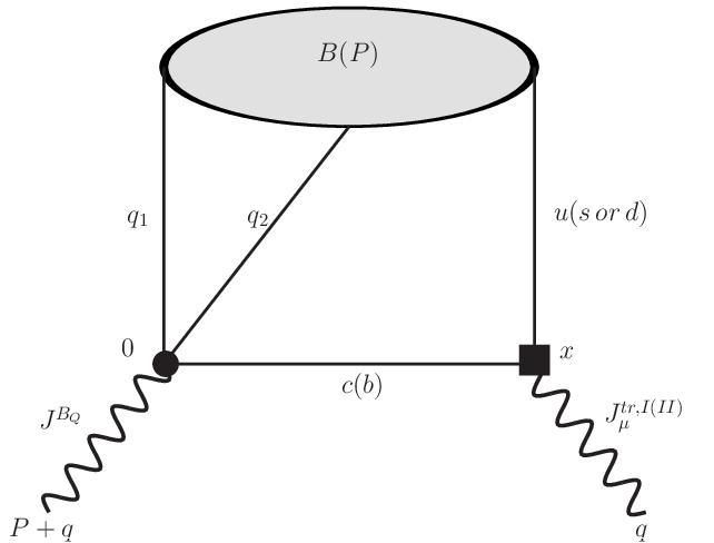
Refer to caption
Refer to caption
Figure 1: Diagrammatic representations of the correlation functions given in Eq. (5). The left (right) diagram belongs to the tree (loop) level transitions. The ovals (wavy lines) in diagrams stand for the DA’s of Ξ\Xi or Σ\Sigma baryons (external currents). In each graph, the q1q_{1} and q2q_{2} are light spectator quarks.

Our main task in the present work is to calculate the transition form factors. According to the philosophy of the QCD sum rules approach, we start with the following correlation functions as the main building blocks of the method:

ΠμI​(p,q)=i​∫d4​x​ei​q​x​⟨B⁡(p)∣T⁡{Jμt​r,I​(x),J¯BQ​(0)}∣0⟩,\displaystyle\Pi^{I}_{\mu}(p,q)=i\int d^{4}xe^{iqx}\langle B(p)\mid T\{J_{\mu}^{tr,I}(x),\bar{J}^{B_{Q}}(0)\}\mid 0\rangle~,
ΠμI​I​(p,q)=i​∫d4​x​ei​q​x​⟨B⁡(p)∣T⁡{Jμt​r,I​I​(x),J¯BQ​(0)}∣0⟩,\displaystyle\Pi^{II}_{\mu}(p,q)=i\int d^{4}xe^{iqx}\langle B(p)\mid T\{J_{\mu}^{tr,II}(x),\bar{J}^{B_{Q}}(0)\}\mid 0\rangle~, (5)

where JBQJ^{B_{Q}} is the interpolating current carrying the quantum numbers of the ΞQ​(ΞQ′)\Xi_{Q}(\Xi^{\prime}_{Q}) baryons. The diagrammatic representations of these correlation functions are presented in Figure 1. The interpolating currents for the considered baryons have the following general forms (see for instance [44]):

JΞQ′\displaystyle J^{\Xi^{\prime}_{Q}}\!\!\! =\displaystyle= −12​ϵa​b​c​{(q1a​T​C​Qb)​γ5​q2c+β⁡(q1a​T​C​γ5​Qb)​q2c−[(Qa​T​C​q2b)​γ5​q1c+β⁡(Qa​T​C​γ5​q2b)​q1c]},\displaystyle\!\!\!-{1\over\sqrt{2}}\epsilon^{abc}\Big\{\Big(q_{1}^{aT}CQ^{b}\Big)\gamma_{5}q_{2}^{c}+\beta\Big(q_{1}^{aT}C\gamma_{5}Q^{b}\Big)q_{2}^{c}-\Big[\Big(Q^{aT}Cq_{2}^{b}\Big)\gamma_{5}q_{1}^{c}+\beta\Big(Q^{aT}C\gamma_{5}q_{2}^{b}\Big)q_{1}^{c}\Big]\Big\}~,
JΞQ\displaystyle J^{\Xi_{Q}}\!\!\! =\displaystyle= 16ϵa​b​c{2(q1a​TCq2b)γ5Qc+2β(q1a​TCγ5q2b)Qc+(q1a​TCQb)γ5q2c+β(q1a​TCγ5Qb)q2c\displaystyle\!\!\!{1\over\sqrt{6}}\epsilon^{abc}\Big\{2\Big(q_{1}^{aT}Cq_{2}^{b}\Big)\gamma_{5}Q^{c}+2\beta\Big(q_{1}^{aT}C\gamma_{5}q_{2}^{b}\Big)Q^{c}+\Big(q_{1}^{aT}CQ^{b}\Big)\gamma_{5}q_{2}^{c}+\beta\Big(q_{1}^{aT}C\gamma_{5}Q^{b}\Big)q_{2}^{c} (6)
+\displaystyle+ (Qa​TCq2b)γ5q1c+β(Qa​TCγ5q2b)q1c},\displaystyle\!\!\!\Big(Q^{aT}Cq_{2}^{b}\Big)\gamma_{5}q_{1}^{c}+\beta\Big(Q^{aT}C\gamma_{5}q_{2}^{b}\Big)q_{1}^{c}\Big\}~,

where CC is the charge conjugation operator, aa, bb and cc are color indices and the light quarks q1q_{1} and q2q_{2} are given in Table 1. The β\beta is an arbitrary parameter and the value β=−1\beta=-1 corresponds to the Ioffe current.

Ξb⁡(c)−(0)\Xi^{-(0)}_{b(c)} Ξb⁡(c)0​(+)\Xi^{0(+)}_{b(c)} Ξb⁡(c)′−(0)\Xi^{\prime-(0)}_{b(c)} Ξb⁡(c)′0​(+)\Xi^{\prime 0(+)}_{b(c)}
q1q_{1} d u d u
q2q_{2} s s s s
Table 1: The light quark contents of the heavy baryons ΞQ\Xi_{Q} and ΞQ′\Xi_{Q}^{\prime}.

The correlation functions given above can be calculated in two different ways. From the phenomenological or physical side, they are calculated inserting complete sets of hadronic states having the same quantum numbers as the chosen interpolating fields. The results of this side appear in terms of hadronic degrees of freedom. On the other side, the QCD or theoretical side of the correlation functions are calculated in terms of the BB baryon DA’s via operator product expansion (OPE). Then, we match these two different representations to relate the hadronic parameters to fundamental QCD degrees of freedom which leads to QCD sum rules for the considered form factors. To suppress contribution of the higher states and continuum, we apply Borel transformation with respect to the initial momentum squared to both sides of the sum rules and use the quark-hadron duality assumption.

Inserting complete set of hadronic state into correlation functions and isolating the contribution of the ground state, we obtain the following representations from physical side:

ΠμI​(p,q)\displaystyle\Pi_{\mu}^{I}(p,q) =\displaystyle= ∑s⟨B⁡(p)∣Jμt​r,I∣BQ​(p+q,s)⟩​⟨BQ​(p+q,s)​∣J¯BQ​(0)∣​0⟩mBQ2−(p+q)2+⋯,\displaystyle\sum_{s}\frac{\langle B(p)\mid J^{tr,I}_{\mu}\mid B_{Q}(p+q,s)\rangle\langle B_{Q}(p+q,s)\mid\bar{J}^{B_{Q}}(0)\mid 0\rangle}{m_{B_{Q}}^{2}-(p+q)^{2}}+\cdots~, (7)
ΠμI​I​(p,q)\displaystyle\Pi_{\mu}^{II}(p,q) =\displaystyle= ∑s⟨B⁡(p)∣Jμt​r,I​I∣BQ​(p+q,s)⟩​⟨BQ​(p+q,s)​∣J¯BQ​(0)∣​0⟩mBQ2−(p+q)2+⋯,\displaystyle\sum_{s}\frac{\langle B(p)\mid J^{tr,II}_{\mu}\mid B_{Q}(p+q,s)\rangle\langle B_{Q}(p+q,s)\mid\bar{J}^{B_{Q}}(0)\mid 0\rangle}{m_{B_{Q}}^{2}-(p+q)^{2}}+\cdots~, (8)

where the ... stands for the contributions of the higher states and continuum. To proceed, besides the transition matrix elements, we need also to know the matrix element ⟨BQ​(p+q,s)∣J¯BQ​(0)∣0⟩\langle B_{Q}(p+q,s)\mid\bar{J}^{B_{Q}}(0)\mid 0\rangle defined in terms of the residue λBQ\lambda_{B_{Q}},

⟨BQ​(p+q,s)∣J¯BQ​(0)∣0⟩=λBQ​u¯BQ​(p+q,s).\displaystyle\langle B_{Q}(p+q,s)\mid\bar{J}^{B_{Q}}(0)\mid 0\rangle=\lambda_{B_{Q}}\bar{u}_{B_{Q}}(p+q,s)~. (9)

Putting all definitions in Eqs. (7) and (8) and using the completeness relation for Dirac particle as

∑suBQ​(p+q,s)​u¯BQ​(p+q,s)=​p+​q+mBQ,\displaystyle\sum_{s}u_{B_{Q}}(p+q,s)\overline{u}_{B_{Q}}(p+q,s)=\not\!p+\not\!q+m_{B_{Q}}~, (10)

we get the following final representations of the correlation functions in physical side:

ΠμI​(p,q)\displaystyle\Pi_{\mu}^{I}(p,q)\!\!\! =\displaystyle= λBQ​uB​(p)mBQ2−(p+q)2{2f1(Q2)pμ+2f2(Q2)pμq+[f2(Q2)+f3(Q2)]qμq\displaystyle\!\!\!\frac{\lambda_{B_{Q}}u_{B}(p)}{m_{B_{Q}}^{2}-(p+q)^{2}}\Big\{2f_{1}(Q^{2})p_{\mu}+2f_{2}(Q^{2})p_{\mu}\not\!q+\Big[f_{2}(Q^{2})+f_{3}(Q^{2})\Big]q_{\mu}\not\!q (11)
+\displaystyle+ 2​g1​(Q2)​pμ​γ5+2​g2​(Q2)​pμ​​q​γ5+[g2​(Q2)+g3​(Q2)]​qμ​​q​γ5\displaystyle\!\!\!2g_{1}(Q^{2})p_{\mu}\gamma_{5}+2g_{2}(Q^{2})p_{\mu}\not\!q\gamma_{5}+\Big[g_{2}(Q^{2})+g_{3}(Q^{2})\vphantom{\int_{0}^{x_{2}}}\Big]q_{\mu}\not\!q\gamma_{5}
+\displaystyle+ other structures}+…,\displaystyle\!\!\!\mbox{\rm other structures}\Big\}+...~,
ΠμI​I​(p,q)\displaystyle\Pi_{\mu}^{II}(p,q)\!\!\! =\displaystyle= λBQ​uB​(p)mBQ2−(p+q)2{2f1T(Q2)pμ+2f2T(Q2)pμq+[f2T(Q2)+f3T(Q2)]qμq\displaystyle\!\!\!\frac{\lambda_{B_{Q}}u_{B}(p)}{m_{B_{Q}}^{2}-(p+q)^{2}}\Big\{2f_{1}^{T}(Q^{2})p_{\mu}+2f_{2}^{T}(Q^{2})p_{\mu}\not\!q+\Big[f_{2}^{T}(Q^{2})+f_{3}^{T}(Q^{2})\Big]q_{\mu}\not\!q (12)
−\displaystyle- 2​g1T​(Q2)​pμ​γ5−2​g2T​(Q2)​pμ​​q​γ5−[g2T​(Q2)+g3T​(Q2)]​qμ​​q​γ5\displaystyle\!\!\!2g_{1}^{T}(Q^{2})p_{\mu}\gamma_{5}-2g_{2}^{T}(Q^{2})p_{\mu}\not\!q\gamma_{5}-\Big[g_{2}^{T}(Q^{2})+g_{3}^{T}(Q^{2})\Big]q_{\mu}\not\!q\gamma_{5}
+\displaystyle+ other structures}+…,\displaystyle\!\!\!\mbox{\rm other structures}\Big\}+...~,

where we choose the represented structures to obtain sum rules for the form factors or their combinations. Here, we should comment that besides the presented structures, there are other structures which one can select to find the form factors. However, our calculations show that the selected structures lead to the more reliable results having good convergence of sum rules, i.e. in the coefficients of the selected structures, contribution of the higher twists is less than those of the lower twists.

Now, we turn our attention to calculate the QCD sides of the aforesaid correlation functions. They are calculated in deep Euclidean region, where −(p+q)2→∞-(p+q)^{2}\rightarrow\infty. Using the explicit expressions of the interpolating currents and contracting out the quark pairs using the Wick’s theorem, we find

ΠμI\displaystyle\Pi^{I}_{\mu} =\displaystyle= i6ϵa​b​c∫d4xe−i​q​x{([2(C)ϕ​η(γ5)ρ​β+(C)ϕ​β(γ5)ρ​η+(C)β​η(γ5)ρ​ϕ]+β[2(Cγ5)ϕ​η(I)ρ​β\displaystyle\frac{i}{\sqrt{6}}\epsilon^{abc}\int d^{4}xe^{-iqx}\Bigg\{\Bigg(\Big[2(C)_{\phi\eta}(\gamma_{5})_{\rho\beta}+(C)_{\phi\beta}(\gamma_{5})_{\rho\eta}+(C)_{\beta\eta}(\gamma_{5})_{\rho\phi}\Big]+\beta\Bigg[2(C\gamma_{5})_{\phi\eta}(I)_{\rho\beta}
+\displaystyle+ (Cγ5)ϕ​β(I)ρ​η+(Cγ5)β​η(I)ρ​ϕ])[γμ(1−γ5)]σ​θ}Sb(−x)β​σ⟨0|sηa(0)sθb(x)uϕc(0)|Ξ(p)⟩,\displaystyle(C\gamma_{5})_{\phi\beta}(I)_{\rho\eta}+(C\gamma_{5})_{\beta\eta}(I)_{\rho\phi}\Bigg]\Bigg)\Big[\gamma_{\mu}(1-\gamma_{5})\Big]_{\sigma\theta}\Bigg\}S_{b}(-x)_{\beta\sigma}\langle 0|s_{\eta}^{a}(0)s_{\theta}^{b}(x)u_{\phi}^{c}(0)|\Xi(p)\rangle~,
ΠμI​I\displaystyle\Pi^{II}_{\mu} =\displaystyle= −i6ϵa​b​c∫d4xe−i​q​x{([2(C)ϕ​η(γ5)ρ​β+(C)ϕ​β(γ5)ρ​η+(C)β​η(γ5)ρ​ϕ]+β[2(Cγ5)ϕ​η(I)ρ​β\displaystyle\frac{-i}{\sqrt{6}}\epsilon^{abc}\int d^{4}xe^{-iqx}\Bigg\{\Bigg(\Big[2(C)_{\phi\eta}(\gamma_{5})_{\rho\beta}+(C)_{\phi\beta}(\gamma_{5})_{\rho\eta}+(C)_{\beta\eta}(\gamma_{5})_{\rho\phi}\Big]+\beta\Bigg[2(C\gamma_{5})_{\phi\eta}(I)_{\rho\beta}
+\displaystyle+ (Cγ5)ϕ​β(I)ρ​η+(Cγ5)β​η(I)ρ​ϕ])[iσμ​νqν(1−γ5)]σ​θ}Sb(−x)β​σ⟨0|sηa(0)sθb(x)uϕc(0)|Ξ(p)⟩,\displaystyle(C\gamma_{5})_{\phi\beta}(I)_{\rho\eta}+(C\gamma_{5})_{\beta\eta}(I)_{\rho\phi}\Bigg]\Bigg)\Big[i\sigma_{\mu\nu}q^{\nu}(1-\gamma_{5})\Big]_{\sigma\theta}\Bigg\}S_{b}(-x)_{\beta\sigma}\langle 0|s_{\eta}^{a}(0)s_{\theta}^{b}(x)u_{\phi}^{c}(0)|\Xi(p)\rangle~,

for Ξb→Ξ​l+​l−\Xi_{b}\rightarrow\Xi l^{+}l^{-},

ΠμI\displaystyle\Pi^{I}_{\mu} =\displaystyle= i6ϵa​b​c∫d4xe−i​q​x{([2(C)ϕ​η(γ5)ρ​β+(C)ϕ​β(γ5)ρ​η+(C)β​η(γ5)ρ​ϕ]+β[2(Cγ5)ϕ​η(I)ρ​β\displaystyle\frac{i}{\sqrt{6}}\epsilon^{abc}\int d^{4}xe^{-iqx}\Bigg\{\Bigg(\Big[2(C)_{\phi\eta}(\gamma_{5})_{\rho\beta}+(C)_{\phi\beta}(\gamma_{5})_{\rho\eta}+(C)_{\beta\eta}(\gamma_{5})_{\rho\phi}\Big]+\beta\Bigg[2(C\gamma_{5})_{\phi\eta}(I)_{\rho\beta}
+\displaystyle+ (Cγ5)ϕ​β(I)ρ​η+(Cγ5)β​η(I)ρ​ϕ])[γμ(1−γ5)]σ​θ}Sb(−x)β​σ⟨0|uηa(0)sθb(x)dϕc(0)|Σ(p)⟩,\displaystyle(C\gamma_{5})_{\phi\beta}(I)_{\rho\eta}+(C\gamma_{5})_{\beta\eta}(I)_{\rho\phi}\Bigg]\Bigg)\Big[\gamma_{\mu}(1-\gamma_{5})\Big]_{\sigma\theta}\Bigg\}S_{b}(-x)_{\beta\sigma}\langle 0|u_{\eta}^{a}(0)s_{\theta}^{b}(x)d_{\phi}^{c}(0)|\Sigma(p)\rangle~,
ΠμI​I\displaystyle\Pi^{II}_{\mu} =\displaystyle= −i6ϵa​b​c∫d4xe−i​q​x{([2(C)ϕ​η(γ5)ρ​β+(C)ϕ​β(γ5)ρ​η+(C)β​η(γ5)ρ​ϕ]+β[2(Cγ5)ϕ​η(I)ρ​β\displaystyle\frac{-i}{\sqrt{6}}\epsilon^{abc}\int d^{4}xe^{-iqx}\Bigg\{\Bigg(\Big[2(C)_{\phi\eta}(\gamma_{5})_{\rho\beta}+(C)_{\phi\beta}(\gamma_{5})_{\rho\eta}+(C)_{\beta\eta}(\gamma_{5})_{\rho\phi}\Big]+\beta\Bigg[2(C\gamma_{5})_{\phi\eta}(I)_{\rho\beta}
+\displaystyle+ (Cγ5)ϕ​β(I)ρ​η+(Cγ5)β​η(I)ρ​ϕ])[iσμ​νqν(1−γ5)]σ​θ}Sb(−x)β​σ⟨0|uηa(0)sθb(x)dϕc(0)|Σ(p)⟩,\displaystyle(C\gamma_{5})_{\phi\beta}(I)_{\rho\eta}+(C\gamma_{5})_{\beta\eta}(I)_{\rho\phi}\Bigg]\Bigg)\Big[i\sigma_{\mu\nu}q^{\nu}(1-\gamma_{5})\Big]_{\sigma\theta}\Bigg\}S_{b}(-x)_{\beta\sigma}\langle 0|u_{\eta}^{a}(0)s_{\theta}^{b}(x)d_{\phi}^{c}(0)|\Sigma(p)\rangle~,

for Ξb→Σ​l+​l−\Xi_{b}\rightarrow\Sigma l^{+}l^{-},

ΠμI\displaystyle\Pi^{I}_{\mu} =\displaystyle= i6ϵa​b​c∫d4xe−i​q​x{([2(C)ϕ​η(γ5)ρ​β+(C)ϕ​β(γ5)ρ​η+(C)β​η(γ5)ρ​ϕ]+β[2(Cγ5)ϕ​η(I)ρ​β\displaystyle\frac{i}{\sqrt{6}}\epsilon^{abc}\int d^{4}xe^{-iqx}\Bigg\{\Bigg(\Big[2(C)_{\phi\eta}(\gamma_{5})_{\rho\beta}+(C)_{\phi\beta}(\gamma_{5})_{\rho\eta}+(C)_{\beta\eta}(\gamma_{5})_{\rho\phi}\Big]+\beta\Bigg[2(C\gamma_{5})_{\phi\eta}(I)_{\rho\beta}
+\displaystyle+ (Cγ5)ϕ​β(I)ρ​η+(Cγ5)β​η(I)ρ​ϕ])[γμ(1−γ5)]σ​θ}Sb(−x)β​σ⟨0|uηa(0)sθb(x)dϕc(0)|Σ(p)⟩,\displaystyle(C\gamma_{5})_{\phi\beta}(I)_{\rho\eta}+(C\gamma_{5})_{\beta\eta}(I)_{\rho\phi}\Bigg]\Bigg)\Big[\gamma_{\mu}(1-\gamma_{5})\Big]_{\sigma\theta}\Bigg\}S_{b}(-x)_{\beta\sigma}\langle 0|u_{\eta}^{a}(0)s_{\theta}^{b}(x)d_{\phi}^{c}(0)|\Sigma(p)\rangle~,
ΠμI​I\displaystyle\Pi^{II}_{\mu} =\displaystyle= −i6ϵa​b​c∫d4xe−i​q​x{([2(C)ϕ​η(γ5)ρ​β+(C)ϕ​β(γ5)ρ​η+(C)β​η(γ5)ρ​ϕ]+β[2(Cγ5)ϕ​η(I)ρ​β\displaystyle\frac{-i}{\sqrt{6}}\epsilon^{abc}\int d^{4}xe^{-iqx}\Bigg\{\Bigg(\Big[2(C)_{\phi\eta}(\gamma_{5})_{\rho\beta}+(C)_{\phi\beta}(\gamma_{5})_{\rho\eta}+(C)_{\beta\eta}(\gamma_{5})_{\rho\phi}\Big]+\beta\Bigg[2(C\gamma_{5})_{\phi\eta}(I)_{\rho\beta}
+\displaystyle+ (Cγ5)ϕ​β(I)ρ​η+(Cγ5)β​η(I)ρ​ϕ])[iσμ​νqν(1−γ5)]σ​θ}Sb(−x)β​σ⟨0|uηa(0)sθb(x)dϕc(0)|Σ(p)⟩,\displaystyle(C\gamma_{5})_{\phi\beta}(I)_{\rho\eta}+(C\gamma_{5})_{\beta\eta}(I)_{\rho\phi}\Bigg]\Bigg)\Big[i\sigma_{\mu\nu}q^{\nu}(1-\gamma_{5})\Big]_{\sigma\theta}\Bigg\}S_{b}(-x)_{\beta\sigma}\langle 0|u_{\eta}^{a}(0)s_{\theta}^{b}(x)d_{\phi}^{c}(0)|\Sigma(p)\rangle~,

for Ξc→Σ​l+​l−\Xi_{c}\rightarrow\Sigma l^{+}l^{-},

ΠμI\displaystyle\Pi^{I}_{\mu} =\displaystyle= −i2ϵa​b​c∫d4xe−i​q​x{([(C)ϕ​β(γ5)ρ​η−(C)β​η(γ5)ρ​ϕ]+β[(Cγ5)ϕ​β(I)ρ​η\displaystyle\frac{-i}{\sqrt{2}}\epsilon^{abc}\int d^{4}xe^{-iqx}\Bigg\{\Bigg(\Big[(C)_{\phi\beta}(\gamma_{5})_{\rho\eta}-(C)_{\beta\eta}(\gamma_{5})_{\rho\phi}\Big]+\beta\Bigg[(C\gamma_{5})_{\phi\beta}(I)_{\rho\eta}
−\displaystyle- (Cγ5)β​η(I)ρ​ϕ])[γμ(1−γ5)]σ​θ}Sb(−x)β​σ⟨0|sηa(0)sθb(x)uϕc(0)|Ξ(p)⟩,\displaystyle(C\gamma_{5})_{\beta\eta}(I)_{\rho\phi}\Bigg]\Bigg)\Big[\gamma_{\mu}(1-\gamma_{5})\Big]_{\sigma\theta}\Bigg\}S_{b}(-x)_{\beta\sigma}\langle 0|s_{\eta}^{a}(0)s_{\theta}^{b}(x)u_{\phi}^{c}(0)|\Xi(p)\rangle~,
ΠμI​I\displaystyle\Pi^{II}_{\mu} =\displaystyle= i2ϵa​b​c∫d4xe−i​q​x{([(C)ϕ​β(γ5)ρ​η−(C)β​η(γ5)ρ​ϕ]+β[(Cγ5)ϕ​β(I)ρ​η\displaystyle\frac{i}{\sqrt{2}}\epsilon^{abc}\int d^{4}xe^{-iqx}\Bigg\{\Bigg(\Big[(C)_{\phi\beta}(\gamma_{5})_{\rho\eta}-(C)_{\beta\eta}(\gamma_{5})_{\rho\phi}\Big]+\beta\Bigg[(C\gamma_{5})_{\phi\beta}(I)_{\rho\eta}
−\displaystyle- (Cγ5)β​η(I)ρ​ϕ])[iσμ​νqν(1−γ5)]σ​θ}Sb(−x)β​σ⟨0|sηa(0)sθb(x)uϕc(0)|Ξ(p)⟩,\displaystyle(C\gamma_{5})_{\beta\eta}(I)_{\rho\phi}\Bigg]\Bigg)\Big[i\sigma_{\mu\nu}q^{\nu}(1-\gamma_{5})\Big]_{\sigma\theta}\Bigg\}S_{b}(-x)_{\beta\sigma}\langle 0|s_{\eta}^{a}(0)s_{\theta}^{b}(x)u_{\phi}^{c}(0)|\Xi(p)\rangle~,

for Ξb′→Ξ​l+​l−\Xi^{\prime}_{b}\rightarrow\Xi l^{+}l^{-},

ΠμI\displaystyle\Pi^{I}_{\mu} =\displaystyle= −i2ϵa​b​c∫d4xe−i​q​x{([(C)ϕ​β(γ5)ρ​η−(C)β​η(γ5)ρ​ϕ]+β[(Cγ5)ϕ​β(I)ρ​η\displaystyle\frac{-i}{\sqrt{2}}\epsilon^{abc}\int d^{4}xe^{-iqx}\Bigg\{\Bigg(\Big[(C)_{\phi\beta}(\gamma_{5})_{\rho\eta}-(C)_{\beta\eta}(\gamma_{5})_{\rho\phi}\Big]+\beta\Bigg[(C\gamma_{5})_{\phi\beta}(I)_{\rho\eta}
−\displaystyle- (Cγ5)β​η(I)ρ​ϕ])[γμ(1−γ5)]σ​θ}Sb(−x)β​σ⟨0|dηa(0)sθb(x)dϕc(0)|Σ(p)⟩,\displaystyle(C\gamma_{5})_{\beta\eta}(I)_{\rho\phi}\Bigg]\Bigg)\Big[\gamma_{\mu}(1-\gamma_{5})\Big]_{\sigma\theta}\Bigg\}S_{b}(-x)_{\beta\sigma}\langle 0|d_{\eta}^{a}(0)s_{\theta}^{b}(x)d_{\phi}^{c}(0)|\Sigma(p)\rangle~,
ΠμI​I\displaystyle\Pi^{II}_{\mu} =\displaystyle= i2ϵa​b​c∫d4xe−i​q​x{([(C)ϕ​β(γ5)ρ​η−(C)β​η(γ5)ρ​ϕ]+β[(Cγ5)ϕ​β(I)ρ​η\displaystyle\frac{i}{\sqrt{2}}\epsilon^{abc}\int d^{4}xe^{-iqx}\Bigg\{\Bigg(\Big[(C)_{\phi\beta}(\gamma_{5})_{\rho\eta}-(C)_{\beta\eta}(\gamma_{5})_{\rho\phi}\Big]+\beta\Bigg[(C\gamma_{5})_{\phi\beta}(I)_{\rho\eta}
−\displaystyle- (Cγ5)β​η(I)ρ​ϕ])[iσμ​νqν(1−γ5)]σ​θ}Sb(−x)β​σ⟨0|dηa(0)sθb(x)dϕc(0)|Σ(p)⟩,\displaystyle(C\gamma_{5})_{\beta\eta}(I)_{\rho\phi}\Bigg]\Bigg)\Big[i\sigma_{\mu\nu}q^{\nu}(1-\gamma_{5})\Big]_{\sigma\theta}\Bigg\}S_{b}(-x)_{\beta\sigma}\langle 0|d_{\eta}^{a}(0)s_{\theta}^{b}(x)d_{\phi}^{c}(0)|\Sigma(p)\rangle~,

for Ξb′→Σ​l+​l−\Xi^{\prime}_{b}\rightarrow\Sigma l^{+}l^{-},

ΠμI\displaystyle\Pi^{I}_{\mu} =\displaystyle= −i2ϵa​b​c∫d4xe−i​q​x{([(C)ϕ​β(γ5)ρ​η−(C)β​η(γ5)ρ​ϕ]+β[(Cγ5)ϕ​β(I)ρ​η\displaystyle\frac{-i}{\sqrt{2}}\epsilon^{abc}\int d^{4}xe^{-iqx}\Bigg\{\Bigg(\Big[(C)_{\phi\beta}(\gamma_{5})_{\rho\eta}-(C)_{\beta\eta}(\gamma_{5})_{\rho\phi}\Big]+\beta\Bigg[(C\gamma_{5})_{\phi\beta}(I)_{\rho\eta}
−\displaystyle- (Cγ5)β​η(I)ρ​ϕ])[γμ(1−γ5)]σ​θ}Sc(−x)β​σ⟨0|uηa(0)sθb(x)dϕc(0)|Σ(p)⟩,\displaystyle(C\gamma_{5})_{\beta\eta}(I)_{\rho\phi}\Bigg]\Bigg)\Big[\gamma_{\mu}(1-\gamma_{5})\Big]_{\sigma\theta}\Bigg\}S_{c}(-x)_{\beta\sigma}\langle 0|u_{\eta}^{a}(0)s_{\theta}^{b}(x)d_{\phi}^{c}(0)|\Sigma(p)\rangle~,
ΠμI​I\displaystyle\Pi^{II}_{\mu} =\displaystyle= i2ϵa​b​c∫d4xe−i​q​x{([(C)ϕ​β(γ5)ρ​η−(C)β​η(γ5)ρ​ϕ]+β[(Cγ5)ϕ​β(I)ρ​η\displaystyle\frac{i}{\sqrt{2}}\epsilon^{abc}\int d^{4}xe^{-iqx}\Bigg\{\Bigg(\Big[(C)_{\phi\beta}(\gamma_{5})_{\rho\eta}-(C)_{\beta\eta}(\gamma_{5})_{\rho\phi}\Big]+\beta\Bigg[(C\gamma_{5})_{\phi\beta}(I)_{\rho\eta}
−\displaystyle- (Cγ5)β​η(I)ρ​ϕ])[iσμ​νqν(1−γ5)]σ​θ}Sc(−x)β​σ⟨0|uηa(0)sθb(x)dϕc(0)|Σ(p)⟩,\displaystyle(C\gamma_{5})_{\beta\eta}(I)_{\rho\phi}\Bigg]\Bigg)\Big[i\sigma_{\mu\nu}q^{\nu}(1-\gamma_{5})\Big]_{\sigma\theta}\Bigg\}S_{c}(-x)_{\beta\sigma}\langle 0|u_{\eta}^{a}(0)s_{\theta}^{b}(x)d_{\phi}^{c}(0)|\Sigma(p)\rangle~,

for Ξc′→Σ​l+​l−\Xi^{\prime}_{c}\rightarrow\Sigma l^{+}l^{-},

Πμ\displaystyle\Pi_{\mu} =\displaystyle= i6ϵa​b​c∫d4xe−i​q​x{[2(C)ϕ​η(γ5)ρ​β+(C)ϕ​β(γ5)ρ​η+(C)β​η(γ5)ρ​ϕ]+β[2(Cγ5)ϕ​η(I)ρ​β\displaystyle\frac{i}{\sqrt{6}}\epsilon^{abc}\int d^{4}xe^{-iqx}\Bigg\{\Big[2(C)_{\phi\eta}(\gamma_{5})_{\rho\beta}+(C)_{\phi\beta}(\gamma_{5})_{\rho\eta}+(C)_{\beta\eta}(\gamma_{5})_{\rho\phi}\Big]+\beta\Bigg[2(C\gamma_{5})_{\phi\eta}(I)_{\rho\beta}
+\displaystyle+ (Cγ5)ϕ​β(I)ρ​η+(Cγ5)β​η(I)ρ​ϕ]}[γμ(1−γ5)]σ​θSc(−x)β​σ⟨0|sηa(0)sθb(x)dϕc(0)|Ξ(p)⟩,\displaystyle(C\gamma_{5})_{\phi\beta}(I)_{\rho\eta}+(C\gamma_{5})_{\beta\eta}(I)_{\rho\phi}\Bigg]\Bigg\}\Big[\gamma_{\mu}(1-\gamma_{5})\Big]_{\sigma\theta}S_{c}(-x)_{\beta\sigma}\langle 0|s_{\eta}^{a}(0)s_{\theta}^{b}(x)d_{\phi}^{c}(0)|\Xi(p)\rangle,

for Ξc→Ξ​l​ν\Xi_{c}\rightarrow\Xi l\nu,

Πμ\displaystyle\Pi_{\mu} =\displaystyle= i6ϵa​b​c∫d4xe−i​q​x{[2(C)ϕ​η(γ5)ρ​β+(C)ϕ​β(γ5)ρ​η+(C)β​η(γ5)ρ​ϕ]+β[2(Cγ5)ϕ​η(I)ρ​β\displaystyle\frac{i}{\sqrt{6}}\epsilon^{abc}\int d^{4}xe^{-iqx}\Bigg\{\Big[2(C)_{\phi\eta}(\gamma_{5})_{\rho\beta}+(C)_{\phi\beta}(\gamma_{5})_{\rho\eta}+(C)_{\beta\eta}(\gamma_{5})_{\rho\phi}\Big]+\beta\Bigg[2(C\gamma_{5})_{\phi\eta}(I)_{\rho\beta}
+\displaystyle+ (Cγ5)ϕ​β(I)ρ​η+(Cγ5)β​η(I)ρ​ϕ]}[γμ(1−γ5)]σ​θSc(−x)β​σ⟨0|uηa(0)sθb(x)dϕc(0)|Σ(p)⟩,\displaystyle(C\gamma_{5})_{\phi\beta}(I)_{\rho\eta}+(C\gamma_{5})_{\beta\eta}(I)_{\rho\phi}\Bigg]\Bigg\}\Big[\gamma_{\mu}(1-\gamma_{5})\Big]_{\sigma\theta}S_{c}(-x)_{\beta\sigma}\langle 0|u_{\eta}^{a}(0)s_{\theta}^{b}(x)d_{\phi}^{c}(0)|\Sigma(p)\rangle,

for Ξc→Σ​l​ν\Xi_{c}\rightarrow\Sigma l\nu,

Πμ\displaystyle\Pi_{\mu} =\displaystyle= −i2​ϵa​b​c​∫d4​x​e−i​q​x​{[(C)ϕ​β​(γ5)ρ​η−(C)β​η​(γ5)ρ​ϕ]+β⁡[(C​γ5)ϕ​β​(I)ρ​η−(C​γ5)β​η​(I)ρ​ϕ]}\displaystyle\frac{-i}{\sqrt{2}}\epsilon^{abc}\int d^{4}xe^{-iqx}\Bigg\{\Big[(C)_{\phi\beta}(\gamma_{5})_{\rho\eta}-(C)_{\beta\eta}(\gamma_{5})_{\rho\phi}\Big]+\beta\Bigg[(C\gamma_{5})_{\phi\beta}(I)_{\rho\eta}-(C\gamma_{5})_{\beta\eta}(I)_{\rho\phi}\Bigg]\Bigg\}
[γμ​(1−γ5)]σ​θ​Sc​(−x)β​σ​⟨0|sηa​(0)​sθb​(x)​uϕc​(0)|Ξ⁡(p)⟩,\displaystyle\Big[\gamma_{\mu}(1-\gamma_{5})\Big]_{\sigma\theta}S_{c}(-x)_{\beta\sigma}\langle 0|s_{\eta}^{a}(0)s_{\theta}^{b}(x)u_{\phi}^{c}(0)|\Xi(p)\rangle,

for Ξc′→Ξ​l​ν\Xi^{\prime}_{c}\rightarrow\Xi l\nu, and

Πμ\displaystyle\Pi_{\mu} =\displaystyle= −i2​ϵa​b​c​∫d4​x​e−i​q​x​{[(C)ϕ​β​(γ5)ρ​η−(C)β​η​(γ5)ρ​ϕ]+β⁡[(C​γ5)ϕ​β​(I)ρ​η−(C​γ5)β​η​(I)ρ​ϕ]}\displaystyle\frac{-i}{\sqrt{2}}\epsilon^{abc}\int d^{4}xe^{-iqx}\Bigg\{\Big[(C)_{\phi\beta}(\gamma_{5})_{\rho\eta}-(C)_{\beta\eta}(\gamma_{5})_{\rho\phi}\Big]+\beta\Bigg[(C\gamma_{5})_{\phi\beta}(I)_{\rho\eta}-(C\gamma_{5})_{\beta\eta}(I)_{\rho\phi}\Bigg]\Bigg\}
[γμ​(1−γ5)]σ​θ​Sc​(−x)β​σ​⟨0|uηa​(0)​sθb​(x)​dϕc​(0)|Σ⁡(p)⟩,\displaystyle\Big[\gamma_{\mu}(1-\gamma_{5})\Big]_{\sigma\theta}S_{c}(-x)_{\beta\sigma}\langle 0|u_{\eta}^{a}(0)s_{\theta}^{b}(x)d_{\phi}^{c}(0)|\Sigma(p)\rangle,

for Ξc′→Σ​l​ν\Xi^{\prime}_{c}\rightarrow\Sigma l\nu, where SQ​(x)S_{Q}(x) is the heavy quark propagator which is given by [45]:

SQ​(x)\displaystyle S_{Q}(x) =\displaystyle= SQf​r​e​e(x)−igs∫d4​k(2​π)4e−i​k​x∫01dv[​k+mQ(mQ2−k2)2Gμ​ν(vx)σμ​ν\displaystyle S_{Q}^{free}(x)-ig_{s}\int\frac{d^{4}k}{(2\pi)^{4}}e^{-ikx}\int_{0}^{1}dv\Bigg[\frac{\not\!k+m_{Q}}{(m_{Q}^{2}-k^{2})^{2}}G^{\mu\nu}(vx)\sigma_{\mu\nu} (29)
+\displaystyle+ 1mQ2−k2vxμGμ​νγν],\displaystyle\!\!\!\frac{1}{m_{Q}^{2}-k^{2}}vx_{\mu}G^{\mu\nu}\gamma_{\nu}\Bigg]~,

and,

SQf​r​e​e\displaystyle S^{free}_{Q}\!\!\! =\displaystyle= mQ24​π2​K1​(mb​−x2)−x2−i​mQ2​​x4​π2​x2​K2​(mb​−x2),\displaystyle\!\!\!\frac{m_{Q}^{2}}{4\pi^{2}}\frac{K_{1}(m_{b}\sqrt{-x^{2}})}{\sqrt{-x^{2}}}-i\frac{m_{Q}^{2}\not\!x}{4\pi^{2}x^{2}}K_{2}(m_{b}\sqrt{-x^{2}})~, (30)

with KiK_{i} being the Bessel functions. In Eq. (29), the SQf​r​e​eS_{Q}^{free} corresponds to the free propagation of the heavy quark. The interaction of the heavy quark with the external gluon field is represented by the remaining terms. However calculation of these types of interactions requires knowledge of the currently unknown four-and five-particle baryonic DA’s. The contribution of such terms are expected to be small [46, 47, 48], hence, in the present work we ignore their contributions.

To complete the calculations in QCD side, we need also the wave functions of the Ξ\Xi and Σ\Sigma baryons, i.e., ϵa​b​c​⟨0|​sηa​(0)​sθb​(x)​uϕc​(0)​|Ξ⁡(p)⟩\epsilon^{abc}\langle 0|s_{\eta}^{a}(0)s_{\theta}^{b}(x)u_{\phi}^{c}(0)|\Xi(p)\rangle and ϵa​b​c​⟨0|u​(d)ηa​(0)​sθb​(x)​dϕc​(0)|Σ⁡(p)⟩\epsilon^{abc}\langle 0|u(d)_{\eta}^{a}(0)s_{\theta}^{b}(x)d_{\phi}^{c}(0)|\Sigma(p)\rangle. These wave functions are expanded in terms of DA’s having different twists which are calculated in [49] and [50]. For completeness, we present the explicit forms of the wave functions together with the DA’s in the Appendix. Using the wave functions and heavy quark propagator we obtain the correlation functions in QCD side.

To obtain sum rules for the form factors, we match the coefficients of the same Dirac structures from both sides of the correlation functions. We also apply Borel transformation and continuum subtraction to suppress the contribution of the higher states and continuum. These processes bring us two auxiliary parameters, namely Borel mass parameter M2M^{2} and continuum threshold s0s_{0} which we will find the working regions for these quantities in the next section. In the meanwhile, we need also the residues λΞQ​(ΞQ′)\lambda_{\Xi_{Q}(\Xi^{\prime}_{Q})} whose explicit forms are given in [24]. The explicit forms of sum rules for the form factors are very lengthy and we do not present their explicit expressions here, but we will give their fit functions in terms of q2q^{2} in next section.

3 Numerical Results

In this section, we numerically analyze the form factors and obtain their behavior in terms of q2q^{2}. Using the fit functions of the form factors, we also calculate the decay rates for all considered channels and branching ratios for the channels in which the lifetime of initial particle is known. Some input parameters used in the numerical calculations are: mΞb0=(5790.5±2.7)m_{\Xi_{b}^{0}}=(5790.5\pm 2.7) MeV, mΞ′b=(5790.5±2.7)m_{\Xi^{{}^{\prime}}_{b}}=(5790.5\pm 2.7) MeV, mΞ0=(1314.86±0.20)m_{\Xi^{0}}=(1314.86\pm 0.20) MeV, mΞc0=(2470.88−0.80+0.34)m_{\Xi_{c}^{0}}=(2470.88^{+0.34}_{-0.80}) MeV, mΞ′⁣+c=(2575.6±3.1)m_{\Xi^{{}^{\prime+}}_{c}}=(2575.6\pm 3.1) MeV, mΞ′0c=(2577.9±2.9)m_{\Xi^{{}^{\prime 0}}_{c}}=(2577.9\pm 2.9) MeV, mΣ0=(1192.642±0.024)m_{\Sigma^{0}}=(1192.642\pm 0.024) MeV, mΣ−=(1197.449±0.030)m_{\Sigma^{-}}=(1197.449\pm 0.030) MeV, mb=(4.7±0.1)m_{b}=(4.7\pm 0.1) GeV, mc=(1.27−0.09+0.07)m_{c}=(1.27^{+0.07}_{-0.09}) GeV, |Vc​s|=1.023±0.036|V_{cs}|=1.023\pm 0.036, |Vc​d|=0.230±0.011|V_{cd}|=0.230\pm 0.011, |Vt​bVtd∗|=8.27×10⁻³|V_{tb}V_{td*}|=8.27\times 10^{-3}, |Vt​bVts∗|=0.041|V_{tb}V_{ts*}|=0.041 , Vb​c=(41.2±1.1)×10−3V_{bc}=(41.2\pm 1.1)\times 10^{-3}, Vb​u=(3.93±0.36)×10−3V_{bu}=(3.93\pm 0.36)\times 10^{-3} [1], C7e​f​f=−0.313C_{7}^{eff}=-0.313, C9e​f​f=4.344C_{9}^{eff}=4.344 and C10=−4.669C_{10}=-4.669 [51].

The main input parameters of the LCSR for form factors are the DA’s of the Ξ\Xi and Σ\Sigma baryons presented in the Appendix. These DA’s contain also four independent parameters. These parameters in the case of Ξ\Xi baryon are given as [49]:

fΞ\displaystyle f_{\Xi} =\displaystyle= (9.9±0.4)×10−3GeV2,λ1=−(2.8±0.1)×10−2GeV2,\displaystyle(9.9\pm 0.4)\times 10^{-3}\;\mbox{GeV}^{2},\hskip 71.13188pt\lambda_{1}=-(2.8\pm 0.1)\times 10^{-2}\;\mbox{GeV}^{2},
λ2\displaystyle\lambda_{2} =\displaystyle= (5.2±0.2)×10−2​GeV2,λ3=(1.7±0.1)×10−2​GeV2,\displaystyle(5.2\pm 0.2)\times 10^{-2}\;\mbox{GeV}^{2},\hskip 71.13188pt\lambda_{3}=(1.7\pm 0.1)\times 10^{-2}\;\mbox{GeV}^{2}, (31)

and for Σ\Sigma baryon, they take the values [50]:

fΣ\displaystyle f_{\Sigma} =\displaystyle= (9.4±0.4)×10−3GeV2,λ1=−(2.5±0.1)×10−2GeV2,\displaystyle(9.4\pm 0.4)\times 10^{-3}\;\mbox{GeV}^{2},\hskip 71.13188pt\lambda_{1}=-(2.5\pm 0.1)\times 10^{-2}\;\mbox{GeV}^{2},
λ2\displaystyle\lambda_{2} =\displaystyle= (4.4±0.1)×10−2​GeV2,λ3=(2.0±0.1)×10−2​GeV2.\displaystyle(4.4\pm 0.1)\times 10^{-2}\;\mbox{GeV}^{2},\hskip 71.13188pt\lambda_{3}=(2.0\pm 0.1)\times 10^{-2}\;\mbox{GeV}^{2}. (32)

The LCSR for form factors contain also three auxiliary parameters. Borel mass parameter M2M^{2} and continuum threshold s0s_{0} are two of them coming from the Borel transformation and continuum subtraction, respectively. The general parameter β\beta is the third parameter entering the calculations from the general form of the interpolating currents for BQB_{Q} baryons. According to the standard criteria in QCD sum rules, the results of form factors should be independent of these auxiliary parameters. Hence, we should look for working regions of these parameters such that the dependence of the results on these parameters are weak. The working region for the Borel mass parameter is determined requiring that not only the higher states and continuum contributions constitute a small percentage of the total dispersion integral but also the series of the light cone expansion with increasing twist should converge. This leads to the interval 15​GeV2≤M2≤30​GeV215~\mbox{GeV}^{2}\leq M^{2}\leq 30~\mbox{GeV}^{2} for bottom baryons and 4​GeV2≤M2≤10​GeV24~\mbox{GeV}^{2}\leq M^{2}\leq 10~\mbox{GeV}^{2} for charmed baryons. The continuum threshold s0s_{0} is not totally arbitrary but it is related to the energy of the first excited state. Our numerical calculations show that in the region (mBQ+0.3)2​GeV2≤s0≤(mBQ+0.7)2​GeV2(m_{B_{Q}}+0.3)^{2}~\mbox{GeV}^{2}\leq s_{0}\leq(m_{B_{Q}}+0.7)^{2}~\mbox{GeV}^{2}, the results of the form factors exhibit very weak dependency on this parameter. Our numerical calculations also lead to the working region −0.6≤cos⁡θ≤0.3-0.6\leq\cos\theta\leq 0.3 with tan⁡θ=β\tan\theta=\beta for the general parameter β\beta. As an example, we present the dependence of the form factor f2f_{2} for Ξb→Ξ​ℓ+​ℓ−\Xi_{b}\rightarrow\Xi\ell^{+}\ell^{-} on cos⁡θ\cos\theta and M2M^{2} in Figures 2 and 3, respectively. From these figures, we see that the form factor f2f_{2} depends weakly on the M2M^{2} and s0s_{0} compared to the cos⁡θ\cos\theta. However, the dependence of the f2f_{2} on cos⁡θ\cos\theta in the above mentioned working region is minimal compared to the intervals out of the working region.

Refer to caption
Figure 2: Form factor f2f_{2} as a function of cos⁡θ\cos\theta for Ξb→Ξ​ℓ+​ℓ−\Xi_{b}\rightarrow\Xi\ell^{+}\ell^{-} decay at q2=13​G​e​V2q^{2}=13~GeV^{2} and working region of M2M^{2} .
Refer to caption
Figure 3: Form factor f2f_{2} as a function of Borel mass parameter M2M^{2} for Ξb→Ξ​l+​l−\Xi_{b}\rightarrow\Xi l^{+}l^{-} decay at q2=13​G​e​V2q^{2}=13~GeV^{2} and working region of β\beta.

Now, we proceed to find the q2q^{2} dependence of the form factors in whole physical region, i.e. 4​mℓ2≤q2≤(mBQ−mB)24m_{\ell}^{2}\leq q^{2}\leq(m_{B_{Q}}-m_{B})^{2} for loop level and mℓ2≤q2≤(mBQ−mB)2m_{\ell}^{2}\leq q^{2}\leq(m_{B_{Q}}-m_{B})^{2} for tree level transitions. However, unfortunately the sum rules for form factors are truncated at some points and are not reliable in the whole physical region. This point for instance for the Ξb→Ξ​l+​l−\Xi_{b}\rightarrow\Xi l^{+}l^{-} transition is roughly at q2=15​G​e​V2q^{2}=15~GeV^{2}. To extend the results to whole physical region, we look for parametrization of the form factors such that in the reliable region, the results obtained from fit parametrization coincide with the sum rules predictions. Using the above working regions for the auxiliary parameters as well as other input parameters, we find that the form factors are well extrapolated by the fit parametrization,

fi​(q2)​[gi​(q2)]=a(1−q2mf​i​t2)+b(1−q2mf​i​t2)2.\displaystyle f_{i}(q^{2})[g_{i}(q^{2})]=\frac{a}{(1-\frac{q^{2}}{m_{fit}^{2}})}+\frac{b}{(1-\frac{q^{2}}{m_{fit}^{2}})^{2}}. (33)

The central values for the fit parameters aa, bb, and mf​i​tm_{fit} as well as values of the form factors at q2=0q^{2}=0 are presented in Tables 7-16. The errors in the values of the form factors at q2=0q^{2}=0 are due to the variation of the auxiliary parameters M2M^{2}, s0s_{0}, and β\beta in their working regions as well as the errors in the other input parameters. To see how the results obtained from the fit function coincide well with the sum rules predictions at reliable region, we depict the dependence of the form factors f2f_{2} and f2Tf_{2}^{T}, as examples, on q2q^{2} in figures 4 and 5. From these figures, we see that the results obtained from the fit parametrization describe well the sum rules results in the reliable region.

Refer to caption
Figure 4: Form factor f2f_{2} as a function of q2q^{2} for Ξb→Ξ​l+​l−\Xi_{b}\rightarrow\Xi l^{+}l^{-} decay at working regions of auxiliary parameters. The boxes show the sum rules predictions and the solid line belongs to the result obtained from fit parametrization.
Refer to caption
Figure 5: Form factor f2Tf^{T}_{2} as a function of q2q^{2} for Ξb→Ξ​l+​l−\Xi_{b}\rightarrow\Xi l^{+}l^{-} decay at working regions of auxiliary parameters. The boxes show the sum rules predictions and the solid line belongs to the result obtained from fit parametrization.

Our last task is to calculate the decay rates and branching ratios of the considered channels using the fit functions of the form factors. Considering the amplitudes of the transitions and definitions of the transition matrix elements in terms of form factors, the differential decay rate for loop level transitions is obtained as [37] :

d​Γd​s=GF2​αe​m2​mBQ8192​π5​|VQ′​Q​VQ′​q∗|2​v​λ​[Θ⁡(s)+13​Δ​(s)],\displaystyle\frac{d\Gamma}{ds}=\frac{G_{F}^{2}\alpha^{2}_{em}m_{B_{Q}}}{8192\pi^{5}}|V_{Q^{\prime}Q}V_{Q^{\prime}q}^{*}|^{2}v\sqrt{\lambda}\,\Bigg[\Theta(s)+\frac{1}{3}\Delta(s)\Bigg]~, (34)

where s=q2/mBQ2s=q^{2}/m^{2}_{B_{Q}}, GF=1.17×10⁻⁵G_{F}=1.17\times 10^{-5} GeV-2, λ=λ⁡(1,r,s)\lambda=\lambda(1,r,s) with λ⁡(a,b,c)=a2+b2+c2−2​a​b−2​a​c−2​b​c\lambda(a,b,c)=a^{2}+b^{2}+c^{2}-2ab-2ac-2bc and v=1−4​mℓ2q2v=\sqrt{1-\frac{4m_{\ell}^{2}}{q^{2}}} is the lepton velocity. The functions Θ⁡(s)\Theta(s) and Δ⁡(s)\Delta(s) are given as:

Θ⁡(s)\displaystyle\Theta(s)\!\!\! =\displaystyle= 32​mℓ2​mBQ4​s​(1+r−s)​(|D3|2+|E3|2)\displaystyle\!\!\!32m_{\ell}^{2}m_{B_{Q}}^{4}s(1+r-s)\left(\left|D_{3}\right|^{2}+\left|E_{3}\right|^{2}\right) (35)
+\displaystyle+ 64​mℓ2​mBQ3​(1−r−s)​Re​[D1∗​E3+D3​E1∗]\displaystyle\!\!\!64m_{\ell}^{2}m_{B_{Q}}^{3}(1-r-s)\,\mbox{\rm Re}[D_{1}^{\ast}E_{3}+D_{3}E_{1}^{\ast}]
+\displaystyle+ 64​mBQ2​r​(6​mℓ2−mBQ2​s)​Re​[D1∗​E1]\displaystyle\!\!\!64m_{B_{Q}}^{2}\sqrt{r}(6m_{\ell}^{2}-m_{B_{Q}}^{2}s){\rm Re}[D_{1}^{\ast}E_{1}]
+\displaystyle+ 64​mℓ2​mBQ3​r​(2​mBQ​s​Re​[D3∗​E3]+(1−r+s)​Re​[D1∗​D3+E1∗​E3])\displaystyle\!\!\!64m_{\ell}^{2}m_{B_{Q}}^{3}\sqrt{r}\Big(2m_{B_{Q}}s{\rm Re}[D_{3}^{\ast}E_{3}]+(1-r+s){\rm Re}[D_{1}^{\ast}D_{3}+E_{1}^{\ast}E_{3}]\Big)
+\displaystyle+ 32mBQ2(2mℓ2+mBQ2s){(1−r+s)mBQrRe[A1∗A2+B1∗B2]\displaystyle\!\!\!32m_{B_{Q}}^{2}(2m_{\ell}^{2}+m_{B_{Q}}^{2}s)\Big\{(1-r+s)m_{B_{Q}}\sqrt{r}\,\mbox{\rm Re}[A_{1}^{\ast}A_{2}+B_{1}^{\ast}B_{2}]
−\displaystyle- mBQ(1−r−s)Re[A1∗B2+A2∗B1]−2r(Re[A1∗B1]+mBQ2sRe[A2∗B2])}\displaystyle\!\!\!m_{B_{Q}}(1-r-s)\,\mbox{\rm Re}[A_{1}^{\ast}B_{2}+A_{2}^{\ast}B_{1}]-2\sqrt{r}\Big(\mbox{\rm Re}[A_{1}^{\ast}B_{1}]+m_{B_{Q}}^{2}s\,\mbox{\rm Re}[A_{2}^{\ast}B_{2}]\Big)\Big\}
+\displaystyle+ 8​mBQ2​{4​mℓ2​(1+r−s)+mBQ2​[(1−r)2−s2]}​(|A1|2+|B1|2)\displaystyle\!\!\!8m_{B_{Q}}^{2}\Big\{4m_{\ell}^{2}(1+r-s)+m_{B_{Q}}^{2}\Big[(1-r)^{2}-s^{2}\Big]\Big\}\left(\left|A_{1}\right|^{2}+\left|B_{1}\right|^{2}\right)
+\displaystyle+ 8​mBQ4​{4​mℓ2​[λ+(1+r−s)​s]+mBQ2​s​[(1−r)2−s2]}​(|A2|2+|B2|2)\displaystyle\!\!\!8m_{B_{Q}}^{4}\Big\{4m_{\ell}^{2}\Big[\lambda+(1+r-s)s\Big]+m_{B_{Q}}^{2}s\Big[(1-r)^{2}-s^{2}\Big]\Big\}\left(\left|A_{2}\right|^{2}+\left|B_{2}\right|^{2}\right)
−\displaystyle- 8​mBQ2​{4​mℓ2​(1+r−s)−mBQ2​[(1−r)2−s2]}​(|D1|2+|E1|2)\displaystyle\!\!\!8m_{B_{Q}}^{2}\Big\{4m_{\ell}^{2}(1+r-s)-m_{B_{Q}}^{2}\Big[(1-r)^{2}-s^{2}\Big]\Big\}\left(\left|D_{1}\right|^{2}+\left|E_{1}\right|^{2}\right)
+\displaystyle+ 8mBQ5sv2{−8mBQsrRe[D2∗E2]+4(1−r+s)rRe[D1∗D2+E1∗E2]\displaystyle\!\!\!8m_{B_{Q}}^{5}sv^{2}\Big\{-8m_{B_{Q}}s\sqrt{r}\,\mbox{\rm Re}[D_{2}^{\ast}E_{2}]+4(1-r+s)\sqrt{r}\,\mbox{\rm Re}[D_{1}^{\ast}D_{2}+E_{1}^{\ast}E_{2}]
−\displaystyle- 4(1−r−s)Re[D1∗E2+D2∗E1]+mBQ[(1−r)2−s2](|D2|2+|E2|2)},\displaystyle\!\!\!4(1-r-s)\,\mbox{\rm Re}[D_{1}^{\ast}E_{2}+D_{2}^{\ast}E_{1}]+m_{B_{Q}}\Big[(1-r)^{2}-s^{2}\Big]\left(\left|D_{2}\right|^{2}+\left|E_{2}\right|^{2}\right)\Big\}~,
Δ⁡(s)\displaystyle\Delta\left(s\right)\!\!\! =\displaystyle= −8​mBQ4​v2​λ​(|A1|2+|B1|2+|D1|2+|E1|2)\displaystyle\!\!\!-8m_{B_{Q}}^{4}v^{2}\lambda\left(\left|A_{1}\right|^{2}+\left|B_{1}\right|^{2}+\left|D_{1}\right|^{2}+\left|E_{1}\right|^{2}\right) (36)
+\displaystyle+ 8​mBQ6​s​v2​λ​(|A2|2+|B2|2+|D2|2+|E2|2),\displaystyle\!\!\!8m_{B_{Q}}^{6}sv^{2}\lambda\Big(\left|A_{2}\right|^{2}+\left|B_{2}\right|^{2}+\left|D_{2}\right|^{2}+\left|E_{2}\right|^{2}\Big)~,

where r=mB2/mBQ2r=m^{2}_{B}/m^{2}_{B_{Q}} and

A1\displaystyle A_{1}\!\!\! =\displaystyle= 1q2​(f1T+g1T)​(−2​mQ​C7)+(f1−g1)​C9e​f​f\displaystyle\!\!\!\frac{1}{q^{2}}\left(f_{1}^{T}+g_{1}^{T}\right)\left(-2m_{Q}C_{7}\right)+\left(f_{1}-g_{1}\right)C_{9}^{eff}
A2\displaystyle A_{2}\!\!\! =\displaystyle= A1​(1→2),\displaystyle\!\!\!A_{1}\left(1\rightarrow 2\right)~,
A3\displaystyle A_{3}\!\!\! =\displaystyle= A1​(1→3),\displaystyle\!\!\!A_{1}\left(1\rightarrow 3\right)~,
B1\displaystyle B_{1}\!\!\! =\displaystyle= A1(g1→−g1;g1T→−g1T),\displaystyle\!\!\!A_{1}\left(g_{1}\rightarrow-g_{1};~g_{1}^{T}\rightarrow-g_{1}^{T}\right)~,
B2\displaystyle B_{2}\!\!\! =\displaystyle= B1​(1→2),\displaystyle\!\!\!B_{1}\left(1\rightarrow 2\right)~,
B3\displaystyle B_{3}\!\!\! =\displaystyle= B1​(1→3),\displaystyle\!\!\!B_{1}\left(1\rightarrow 3\right)~,
D1\displaystyle D_{1}\!\!\! =\displaystyle= (f1−g1)​C10,\displaystyle\!\!\!\left(f_{1}-g_{1}\right)C_{10}~,
D2\displaystyle D_{2}\!\!\! =\displaystyle= D1​(1→2),\displaystyle\!\!\!D_{1}\left(1\rightarrow 2\right)~,
D3\displaystyle D_{3}\!\!\! =\displaystyle= D1​(1→3),\displaystyle\!\!\!D_{1}\left(1\rightarrow 3\right)~,
E1\displaystyle E_{1}\!\!\! =\displaystyle= D1​(g1→−g1),\displaystyle\!\!\!D_{1}\left(g_{1}\rightarrow-g_{1}\right)~,
E2\displaystyle E_{2}\!\!\! =\displaystyle= E1​(1→2),\displaystyle\!\!\!E_{1}\left(1\rightarrow 2\right)~,
E3\displaystyle E_{3}\!\!\! =\displaystyle= E1​(1→3).\displaystyle\!\!\!E_{1}\left(1\rightarrow 3\right)~. (37)

Integrating the differential decay rate over ss in whole physical region, 4​mℓ2/mBQ2≤s≤(1−r)24m_{\ell}^{2}/m^{2}_{B_{Q}}\leq s\leq(1-\sqrt{r})^{2}, one can obtain the total decay rate.

For the tree level transitions, the formula for the decay width is given by [52, 53]:

Γ=GF2384π3mΞ(′)c3​|Vcs⁡(d)|2​∫ml2δ2d​q2​(1−ml2/q2)2​(σ2−q2)​(δ2−q2)​N​(q2)\displaystyle\Gamma=\frac{G_{F}^{2}}{384\pi^{3}m_{\Xi^{(^{\prime})}_{c}}^{3}}\ |V_{\rm cs(d)}|^{2}\,\,\int\limits_{m_{l}^{2}}^{\delta^{2}}dq^{2}\ (1-m_{l}^{2}/q^{2})^{2}\ \sqrt{(\sigma^{2}-q^{2})(\delta^{2}-q^{2})}\ N(q^{2}) (38)

where

N⁡(q2)\displaystyle N(q^{2}) =\displaystyle= F12​(q2)​(δ2​(4​q2−ml2)+2​σ2​δ2​(1+2​ml2/q2)−(σ2+2​q2)​(2​q2+ml2))\displaystyle F_{1}^{2}(q^{2})(\delta^{2}(4q^{2}-m_{l}^{2})+2\sigma^{2}\delta^{2}(1+2m_{l}^{2}/q^{2})-(\sigma^{2}+2q^{2})(2q^{2}+m_{l}^{2}))
+\displaystyle+ F22(q2)(δ2−q2)(2σ2+q2)(2q2+ml2)/mΞ(′)c2+3F32(q2)ml2(σ2−q2)q2/mΞ(′)c2\displaystyle F_{2}^{2}(q^{2})(\delta^{2}-q^{2})(2\sigma^{2}+q^{2})(2q^{2}+m_{l}^{2})/m_{\Xi^{(^{\prime})}_{c}}^{2}+3F_{3}^{2}(q^{2})m_{l}^{2}(\sigma^{2}-q^{2})q^{2}/m_{\Xi^{(^{\prime})}_{c}}^{2}
+\displaystyle+ 6F1(q2)F2(q2)(δ2−q2)(2q2+ml2)σ/mΞ(′)c−6F1(q2)F3(q2)ml2(σ2−q2)δ/mΞ(′)c\displaystyle 6F_{1}(q^{2})F_{2}(q^{2})(\delta^{2}-q^{2})(2q^{2}+m_{l}^{2})\sigma/m_{\Xi^{(^{\prime})}_{c}}-6F_{1}(q^{2})F_{3}(q^{2})m_{l}^{2}(\sigma^{2}-q^{2})\delta/m_{\Xi^{(^{\prime})}_{c}}
+\displaystyle+ G12​(q2)​(σ2​(4​q2−ml2)+2​σ2​δ2​(1+2​ml2/q2)−(δ2+2​q2)​(2​q2+ml2))\displaystyle G_{1}^{2}(q^{2})(\sigma^{2}(4q^{2}-m_{l}^{2})+2\sigma^{2}\delta^{2}(1+2m_{l}^{2}/q^{2})-(\delta^{2}+2q^{2})(2q^{2}+m_{l}^{2}))
+\displaystyle+ G22(q2)(σ2−q2)(2δ2+q2)(2q2+ml2)/mΞ(′)c2+3G32(q2)ml2(δ2−q2)q2/mΞ(′)c2\displaystyle G_{2}^{2}(q^{2})(\sigma^{2}-q^{2})(2\delta^{2}+q^{2})(2q^{2}+m_{l}^{2})/m_{\Xi^{(^{\prime})}_{c}}^{2}+3G_{3}^{2}(q^{2})m_{l}^{2}(\delta^{2}-q^{2})q^{2}/m_{\Xi^{(^{\prime})}_{c}}^{2}
−\displaystyle- 6G1(q2)G2(q2)(σ2−q2)(2q2+ml2)δ/mΞ(′)c+6G1(q2)G3(q2)ml2(δ2−q2)σ/mΞ(′)c,\displaystyle 6G_{1}(q^{2})G_{2}(q^{2})(\sigma^{2}-q^{2})(2q^{2}+m_{l}^{2})\delta/m_{\Xi^{(^{\prime})}_{c}}+6G_{1}(q^{2})G_{3}(q^{2})m_{l}^{2}(\delta^{2}-q^{2})\sigma/m_{\Xi^{(^{\prime})}_{c}}\,,

with F1​(q2)=f1​(q2)F_{1}(q^{2})=f_{1}(q^{2}), F2(q2)=mΞ(′)cf2(q2)F_{2}(q^{2})=m_{\Xi^{(^{\prime})}_{c}}f_{2}(q^{2}), F3(q2)=mΞ(′)cf3(q2)F_{3}(q^{2})=m_{\Xi^{(^{\prime})}_{c}}f_{3}(q^{2}), G1​(q2)=g1​(q2)G_{1}(q^{2})=g_{1}(q^{2}), G2(q2)=mΞ(′)cg2(q2)G_{2}(q^{2})=m_{\Xi^{(^{\prime})}_{c}}g_{2}(q^{2}), G3(q2)=mΞ(′)cg3(q2)G_{3}(q^{2})=m_{\Xi^{(^{\prime})}_{c}}g_{3}(q^{2}), σ=mΞ(′)c+mB\sigma=m_{\Xi^{(^{\prime})}_{c}}+m_{B}, δ=mΞ(′)c−mB\delta=m_{\Xi^{(^{\prime})}_{c}}-m_{B} and mlm_{l} is the lepton’s mass. The numerical results of decay width for considered channels are presented in Table 17. Finally, for the channels which we know the lifetime of the initial particles [1], we calculate the branching ratios as presented in Table 18. The orders of branching fractions for most of the channels presented in Table 18 show that these channels are accessible at LHC.

4 Conclusion

In the present study, we have considered various loop level and tree level semileptonic decays of heavy Ξb⁡(c)′\Xi^{\prime}_{b(c)} and Ξb⁡(c)\Xi_{b(c)} baryons to the light Ξ\Xi and Σ\Sigma baryons in the framework of the light cone QCD sum rules. The most general form of the interpolating currents for the considered heavy baryons as well as the recently available distribution amplitudes of the Ξ\Xi and Σ\Sigma baryons have been used to calculate twelve form factors for loop level and six form factors for tree level transitions in full theory of QCD. Using the sum rules for the form factors, then, we have evaluated the decay rates of the related transitions. For those transitions with known lifetime, we have also calculated their branching fractions. The orders of branching fractions for tree level Ξc→Σ​l+​νl\Xi_{c}\rightarrow\Sigma~l^{+}\nu_{l} and Ξc→Ξ​l+​νl\Xi_{c}\rightarrow\Xi~l^{+}\nu_{l} (with l=el=e or μ\mu) as well as rare loop level Ξb→Ξ​l+​l−\Xi_{b}\rightarrow\Xi~l^{+}l^{-} and Ξb→Σ​l+​l−\Xi_{b}\rightarrow\Sigma~l^{+}l^{-} (with l=el=e or μ\mu or τ\tau) transitions show that these channels can be detected at LHC. The similar baryonic Λb→Λ​μ+​μ−\Lambda_{b}\rightarrow\Lambda~\mu^{+}\mu^{-} has been observed very recently by CDF Collaboration [54] and they reported the branching ratio of [1.73±0.42([1.73\pm 0.42(statOPEN)±0.55​(CLOSE)\pm 0.55(syst)]×10−6)]\times 10^{-6} which is in good consistency with our previous work [37]. Any measurement on the considered channels in the present work and comparison of the obtained data with our results can help us understand better the internal structures of the considered heavy baryons as well as obtain useful information about the distribution amplitudes of the Ξ\Xi and Σ\Sigma baryons. Such comparison in FCNC channels can help us also in the course of searching for new physics effects beyond the SM.

5 Acknowledgment

Two of the authors (K. A. and H. S.) would like to thank TUBITAK, for their partial financial support provided under the project No.110T284.

References

  • [1] K. Nakamura et al., J. Phys. G 37 , (2010) 075021.
  • [2] A. G. Grozin, O. I. Yakovlev, Phys. Lett. B 285 (1992) 254; Y. B. Dai, C. S. Huang, C. Liu, C. D. Lu, Phys. Lett. B 371 (1996) 99; D. W. Wang, M. Q. Huang, C. Z. Li, Phys. Rev. D 65 (2002) 094036.
  • [3] D. W. Wang, M. Q. Huang, Phys. Rev. D 68 (2003) 034019; Z. G. Wang, Eur. Phys. J. C 54 (2008) 231; F. O. Duraes, M. Nielsen, Phys. Lett. B 658 (2007) 40; X. Liu, H. X. Chen, Y. R. Liu, A. Hosaka, S. L. Zhu, Phys. Rev. D 77 (2008) 014031.
  • [4] E. V. Shuryak, Nucl. Phys. B 198 (1982) 83.
  • [5] Zhi-Gang Wang, Phys. Lett. B 685 (2010) 59.
  • [6] T. M. Aliev, K. Azizi, A. Ozpineci, Nucl. Phys. B 808, (2009) 137.
  • [7] M. Karliner, H. J. Lipkin, Phys. Lett. B 660 (2008) 539.
  • [8] M. Karliner, B. Kereu-Zura, H. J. Lipkin, J. L. Rosner, arXiv:0706.2163 [hep-ph].
  • [9] D. Ebert, R. N. Faustov, V. O. Galkin, Phys. Rev. D 72 (2005) 034026.
  • [10] N. Mathur, R. Lewis , R. M. Woloshyn, Phys. Rev. D 66 (2002) 014502.
  • [11] J. L. Rosner, Phys. Rev. D 75 (2007) 013009.
  • [12] Qiao-Yan Zhao, Dan Zhang, Qiu-Yang Zhang, Chin. Phys. Lett. 28, (2011) 071201.
  • [13] A. L. Choudhury, V. Joshi, Phys. Rev. D 13 (1976) 3115.
  • [14] D. B. Lichtenberg, Phys. Rev. D 15 (1977) 345.
  • [15] R. J. Johnson, M. Shah-Jahan, Phys. Rev. D 15 (1977) 1400.
  • [16] S. K. Bose, L. P. Singh, Phys. Rev. D 22 (1980) 773.
  • [17] L. Y. Glozman, D. O. Riska, Nucl. Phys. A 603 (1996) 326.
  • [18] B. Julia-Diaz, D. O. Riska, Nucl. Phys. A 739 (2004) 69.
  • [19] S. Scholl, H. Weigel, Nucl. Phys. A 735 (2004) 163.
  • [20] Y. S. Oh, B. Y. Park, Mod. Phys. Lett. A 11 (1996) 653.
  • [21] A. Faessler et. al, Phys. Rev. D 73 (2006) 094013.
  • [22] S. L. Zhu, W. Y. Hwang, Z. S. Yang, Phys. Rev. D 56 (1997) 7273.
  • [23] T. M. Aliev, K. Azizi, A. Ozpineci, Phys. Rev. D 77 (2008) 114006.
  • [24] T. M. Aliev, K. Azizi, A. Ozpineci, Phys. Rev. D 79, (2009) 056005.
  • [25] T. M. Aliev, K. Azizi, M. Savci, Phys. Lett. B 696 (2011) 220.
  • [26] T. M. Aliev, K. Azizi, M. Savci, Nucl. Phys. A 852 (2011) 141
  • [27] T. M. Aliev, K. Azizi, M. Savci, V. S. Zamiralov, Phys. Rev. D 83, (2011) 096007.
  • [28] G. Buchalla, G. Hiller and G. Isidori, Phys. Rev. D 63 (2000) 014015.
  • [29] C. Bird, P. Jackson, R. Kowalewski, M. Pospelov, Phys. Rev. Lett. 93 (2004) 201803.
  • [30] D. Ebert, R. N. Faustov, and V. O. Galkin, Phys. Rev. D 73, (2006) 094002.
  • [31] Ming-Qiu Huang, Dao-Wei Wang, Phys. Rev. D 69, (2004) 094003; arXiv:0608170v2 (hep-ph).
  • [32] C. Albertus, E. Hernandez, and J. Nieves, Phys. Rev. D 71, (2005) 014012.
  • [33] Ruben Flores-Mendieta, J.J. Torres, M. Neri, A. Martinez, A. Garcia, Phys. Rev. D 71, (2005) 034023.
  • [34] Muslema Pervin, Winston Roberts, and Simon Capstick, Phys. Rev. C 72, (2005) 035201.
  • [35] K. Azizi, M. Bayar, A. Ozpineci, Y. Sarac, Phys. Rev. D 80, (2009) 036007.
  • [36] K. Azizi, M. Bayar, Y. Sarac, H. Sundu, Phys. Rev. D 80, (2009) 096007.
  • [37] T. M. Aliev, K. Azizi, M. Savci, Phys. Rev. D 81, (2010) 056006.
  • [38] K. Azizi, M. Bayar, M. T. Zeyrek, J. Phys. G: Nucl. Part. Phys. 37, (2010) 085002.
  • [39] T. Mannel, W. Roberts and Z. Ryzak, Nucl. Phys. B 355 (1991) 38.
  • [40] T. M. Aliev, A. Ozpineci, M. Savci, Phys. Rev. D 65 (2002) 115002.
  • [41] M. A. Shifman, A. I. Vainshtein and V. I. Zakharov, Nucl. Phys. B 147, 385 (1979).
  • [42] M. A. Shifman, A. I. Vainstein, V. I. Zakharov, Nucl. Phys. B 147, 448 (1979).
  • [43] I. I. Balitsky, V. M. Braun, A. V. Kolesnichenko, Nucl. Phys. B 312 (1989) 509.
  • [44] E. Bagan, M. Chabab, H. G. Dosch, S. Narison, Phys. Lett. B 278, (1992) 369.
  • [45] I. I. Balitsky, V. M. Braun, Nucl. Phys. B 311 (1989) 541.
  • [46] V. M. Braun, A. Lenz, M. Wittmann, Phys. Rev. D 73 (2006) 094019.
  • [47] V. M. Braun, A. Lenz, N. Mahnke, E. Stein, Phys. Rev. D 65 (2002) 074011; A. Lenz, M. Wittmann and E. Stein, Phys. Lett. B 581, 199 (2004).
  • [48] V. Braun, R. J. Fries, N. Mahnke and E. Stein, Nucl. Phys. B 589 (2000) 381.
  • [49] Yong-Lu Liu, Ming-Qiu Huang, Phys. Rev. D 80, (2009) 055015.
  • [50] Y. L. Liu, M. Q. Huang, Nucl. Phys. A 821, (2009) 80.
  • [51] A. J. Buras, M. Muenz Phys. Rev. D52 (1995) 186.
  • [52] A. Faessler, T. Gutsche, B. R. Holstein, M. A. Ivanov, J. G. Korner, V. E. Lyubovitskij, Phys. Rev. D 78, (2008) 094005.
  • [53] H. Pietschmann, Acta Phys. Austriaca Suppl. 12, (1974) 1.
  • [54] T. Aaltonen et al. (CDF Collaboration), Phys. Rev. Lett. 107, 201802 (2011).

Appendix A

In this Appendix, we present the general decomposition of the wave functions of the baryons in final states, i.e., ϵa​b​c​⟨0|​q1ηa​(0)​q2θb​(x)​q3ϕc​(0)​|B⁡(p)⟩\epsilon^{abc}\langle 0|{q_{1}}_{\eta}^{a}(0){q_{2}}_{\theta}^{b}(x){q_{3}}_{\phi}^{c}(0)|B(p)\rangle and DA’s of the Ξ\Xi and Σ\Sigma baryons [49, 50]:

4​⟨0|ϵa​b​c​q1αa​(a1​x)​q2βb​(a2​x)​q3γc​(a3​x)|B⁡(p)⟩\displaystyle 4\langle 0|\epsilon^{abc}{q_{1}}_{\alpha}^{a}(a_{1}x){q_{2}}_{\beta}^{b}(a_{2}x){q_{3}}_{\gamma}^{c}(a_{3}x)|B(p)\rangle
=\displaystyle= 𝒮1​mB​Cα​β​(γ5​B)γ+𝒮2​mB2​Cα​β​(/​x​γ5​B)γ\displaystyle\!\!\!\mathcal{S}_{1}m_{B}C_{\alpha\beta}(\gamma_{5}B)_{\gamma}+\mathcal{S}_{2}m_{B}^{2}C_{\alpha\beta}(\hbox to0.0pt{/\hss}x\gamma_{5}B)_{\gamma}
+\displaystyle+ 𝒫1​mB​(γ5​C)α​β​Bγ+𝒫2​mB2​(γ5​C)α​β​(/​x​B)γ+(𝒱1+x2​mB24​𝒱1M)​(/​p​C)α​β​(γ5​B)γ\displaystyle\!\!\!\mathcal{P}_{1}m_{B}(\gamma_{5}C)_{\alpha\beta}B_{\gamma}+\mathcal{P}_{2}m_{B}^{2}(\gamma_{5}C)_{\alpha\beta}(\hbox to0.0pt{/\hss}xB)_{\gamma}+(\mathcal{V}_{1}+\frac{x^{2}m_{B}^{2}}{4}\mathcal{V}_{1}^{M})(\hbox to0.0pt{/\hss}pC)_{\alpha\beta}(\gamma_{5}B)_{\gamma}
+\displaystyle+ 𝒱2​mB​(/​p​C)α​β​(/​x​γ5​B)γ+𝒱3​mB​(γμ​C)α​β​(γμ​γ5​B)γ+𝒱4​mB2​(/​x​C)α​β​(γ5​B)γ\displaystyle\!\!\!\mathcal{V}_{2}m_{B}(\hbox to0.0pt{/\hss}pC)_{\alpha\beta}(\hbox to0.0pt{/\hss}x\gamma_{5}B)_{\gamma}+\mathcal{V}_{3}m_{B}(\gamma_{\mu}C)_{\alpha\beta}(\gamma^{\mu}\gamma_{5}B)_{\gamma}+\mathcal{V}_{4}m_{B}^{2}(\hbox to0.0pt{/\hss}xC)_{\alpha\beta}(\gamma_{5}B)_{\gamma}
+\displaystyle+ 𝒱5​mB2​(γμ​C)α​β​(i​σμ​ν​xν​γ5​B)γ+𝒱6​mB3​(/​x​C)α​β​(/​x​γ5​B)γ+(𝒜1CLOSE\displaystyle\!\!\!\mathcal{V}_{5}m_{B}^{2}(\gamma_{\mu}C)_{\alpha\beta}(i\sigma^{\mu\nu}x_{\nu}\gamma_{5}B)_{\gamma}+\mathcal{V}_{6}m_{B}^{3}(\hbox to0.0pt{/\hss}xC)_{\alpha\beta}(\hbox to0.0pt{/\hss}x\gamma_{5}B)_{\gamma}+(\mathcal{A}_{1}
+\displaystyle+ OPENx2​mB24​𝒜1M)​(/​p​γ5​C)α​β​Bγ+𝒜2​mB​(/​p​γ5​C)α​β​(/​x​B)γ+𝒜3​mB​(γμ​γ5​C)α​β​(γμ​B)γ\displaystyle\!\!\!\frac{x^{2}m_{B}^{2}}{4}\mathcal{A}_{1}^{M})(\hbox to0.0pt{/\hss}p\gamma_{5}C)_{\alpha\beta}B_{\gamma}+\mathcal{A}_{2}m_{B}(\hbox to0.0pt{/\hss}p\gamma_{5}C)_{\alpha\beta}(\hbox to0.0pt{/\hss}xB)_{\gamma}+\mathcal{A}_{3}m_{B}(\gamma_{\mu}\gamma_{5}C)_{\alpha\beta}(\gamma^{\mu}B)_{\gamma}
+\displaystyle+ 𝒜4​mB2​(/​x​γ5​C)α​β​Bγ+𝒜5​mB2​(γμ​γ5​C)α​β​(i​σμ​ν​xν​B)γ+𝒜6​mB3​(/​x​γ5​C)α​β​(/​x​B)γ\displaystyle\!\!\!\mathcal{A}_{4}m_{B}^{2}(\hbox to0.0pt{/\hss}x\gamma_{5}C)_{\alpha\beta}B_{\gamma}+\mathcal{A}_{5}m_{B}^{2}(\gamma_{\mu}\gamma_{5}C)_{\alpha\beta}(i\sigma^{\mu\nu}x_{\nu}B)_{\gamma}+\mathcal{A}_{6}m_{B}^{3}(\hbox to0.0pt{/\hss}x\gamma_{5}C)_{\alpha\beta}(\hbox to0.0pt{/\hss}xB)_{\gamma}
+\displaystyle+ (𝒯1+x2​mB24​𝒯1M)​(pν​i​σμ​ν​C)α​β​(γμ​γ5​B)γ+𝒯2​mB​(xμ​pν​i​σμ​ν​C)α​β​(γ5​B)γ\displaystyle\!\!\!(\mathcal{T}_{1}+\frac{x^{2}m_{B}^{2}}{4}\mathcal{T}_{1}^{M})(p^{\nu}i\sigma_{\mu\nu}C)_{\alpha\beta}(\gamma^{\mu}\gamma_{5}B)_{\gamma}+\mathcal{T}_{2}m_{B}(x^{\mu}p^{\nu}i\sigma_{\mu\nu}C)_{\alpha\beta}(\gamma_{5}B)_{\gamma}
+\displaystyle+ 𝒯3​mB​(σμ​ν​C)α​β​(σμ​ν​γ5​B)γ+𝒯4​mB​(pν​σμ​ν​C)α​β​(σμ​ρ​xρ​γ5​B)γ\displaystyle\!\!\!\mathcal{T}_{3}m_{B}(\sigma_{\mu\nu}C)_{\alpha\beta}(\sigma^{\mu\nu}\gamma_{5}B)_{\gamma}+\mathcal{T}_{4}m_{B}(p^{\nu}\sigma_{\mu\nu}C)_{\alpha\beta}(\sigma^{\mu\rho}x_{\rho}\gamma_{5}B)_{\gamma}
+\displaystyle+ 𝒯5​mB2​(xν​i​σμ​ν​C)α​β​(γμ​γ5​B)γ+𝒯6​mB2​(xμ​pν​i​σμ​ν​C)α​β​(/​x​γ5​B)γ\displaystyle\!\!\!\mathcal{T}_{5}m_{B}^{2}(x^{\nu}i\sigma_{\mu\nu}C)_{\alpha\beta}(\gamma^{\mu}\gamma_{5}B)_{\gamma}+\mathcal{T}_{6}m_{B}^{2}(x^{\mu}p^{\nu}i\sigma_{\mu\nu}C)_{\alpha\beta}(\hbox to0.0pt{/\hss}x\gamma_{5}B)_{\gamma}
+\displaystyle+ 𝒯7​mB2​(σμ​ν​C)α​β​(σμ​ν​/​x​γ5​B)γ+𝒯8​mB3​(xν​σμ​ν​C)α​β​(σμ​ρ​xρ​γ5​B)γ.(A​.1)\displaystyle\!\!\!\mathcal{T}_{7}m_{B}^{2}(\sigma_{\mu\nu}C)_{\alpha\beta}(\sigma^{\mu\nu}\hbox to0.0pt{/\hss}x\gamma_{5}B)_{\gamma}+\mathcal{T}_{8}m_{B}^{3}(x^{\nu}\sigma_{\mu\nu}C)_{\alpha\beta}(\sigma^{\mu\rho}x_{\rho}\gamma_{5}B)_{\gamma}~.~~~~~~~~~~~~~~~~~~~~~~~(A.1)

The calligraphic functions in the above expression have not definite twists but they can be written in terms of the BB distribution amplitudes (DA’s) with definite and increasing twists via the scalar product p​xpx. The relationship between the calligraphic functions appearing in the above equation and scalar, pseudo-scalar, vector, axial vector and tensor DA’s for B baryon are given in Tables 2, 3, 4, 5 and 6, respectively.

𝒮1=S1\mathcal{S}_{1}=S_{1}
2​p​x​𝒮2=S1−S22px\mathcal{S}_{2}=S_{1}-S_{2}
Table 2: Relations between the calligraphic functions and B scalar DA’s.
𝒫1=P1\mathcal{P}_{1}=P_{1}
2​p​x​𝒫2=P1−P22px\mathcal{P}_{2}=P_{1}-P_{2}
Table 3: Relations between the calligraphic functions and B pseudo-scalar DA’s.
𝒱1=V1\mathcal{V}_{1}=V_{1}
2​p​x​𝒱2=V1−V2−V32px\mathcal{V}_{2}=V_{1}-V_{2}-V_{3}
2​𝒱3=V32\mathcal{V}_{3}=V_{3}
4​p​x​𝒱4=−2​V1+V3+V4+2​V54px\mathcal{V}_{4}=-2V_{1}+V_{3}+V_{4}+2V_{5}
4​p​x​𝒱5=V4−V34px\mathcal{V}_{5}=V_{4}-V_{3}
4​(p​x)2​𝒱6=−V1+V2+V3+V4+V5−V64(px)^{2}\mathcal{V}_{6}=-V_{1}+V_{2}+V_{3}+V_{4}+V_{5}-V_{6}
Table 4: Relations between the calligraphic functions and B vector DA’s.
𝒜1=A1\mathcal{A}_{1}=A_{1}
2​p​x​𝒜2=−A1+A2−A32px\mathcal{A}_{2}=-A_{1}+A_{2}-A_{3}
2​𝒜3=A32\mathcal{A}_{3}=A_{3}
4​p​x​𝒜4=−2​A1−A3−A4+2​A54px\mathcal{A}_{4}=-2A_{1}-A_{3}-A_{4}+2A_{5}
4​p​x​𝒜5=A3−A44px\mathcal{A}_{5}=A_{3}-A_{4}
4​(p​x)2​𝒜6=A1−A2+A3+A4−A5+A64(px)^{2}\mathcal{A}_{6}=A_{1}-A_{2}+A_{3}+A_{4}-A_{5}+A_{6}
Table 5: Relations between the calligraphic functions and B axial vector DA’s.
𝒯1=T1\mathcal{T}_{1}=T_{1}
2​p​x​𝒯2=T1+T2−2​T32px\mathcal{T}_{2}=T_{1}+T_{2}-2T_{3}
2​𝒯3=T72\mathcal{T}_{3}=T_{7}
2​p​x​𝒯4=T1−T2−2​T72px\mathcal{T}_{4}=T_{1}-T_{2}-2T_{7}
2​p​x​𝒯5=−T1+T5+2​T82px\mathcal{T}_{5}=-T_{1}+T_{5}+2T_{8}
4​(p​x)2​𝒯6=2​T2−2​T3−2​T4+2​T5+2​T7+2​T84(px)^{2}\mathcal{T}_{6}=2T_{2}-2T_{3}-2T_{4}+2T_{5}+2T_{7}+2T_{8}
4​p​x​𝒯7=T7−T84px\mathcal{T}_{7}=T_{7}-T_{8}
4​(p​x)2​𝒯8=−T1+T2+T5−T6+2​T7+2​T84(px)^{2}\mathcal{T}_{8}=-T_{1}+T_{2}+T_{5}-T_{6}+2T_{7}+2T_{8}
Table 6: Relations between the calligraphic functions and B tensor DA’s.

Every distribution amplitude, FF= S1,2S_{1,2}, P1,2P_{1,2}, V1→6V_{1\rightarrow 6}, A1→6A_{1\rightarrow 6}, T1→8T_{1\rightarrow 8} can be represented as:

F⁡(ai​p​x)=∫d​x1​d​x2​d​x3​δ​(x1+x2+x3−1)​e−i​p​x​(∑j=13xj​aj)​F​(xi).(A​.2)\displaystyle F(a_{i}px)=\int dx_{1}dx_{2}dx_{3}\delta(x_{1}+x_{2}+x_{3}-1)e^{-ipx(\sum_{j=1}^{3}~x_{j}a_{j})}F(x_{i})~.~~~~~~~~~~~~~~~~~~~~~~~~~~~~~~(A.2)

where, xix_{i} with i=1,2i=1,~2 or 33 are longitudinal momentum fractions carried by the participating quarks.

The explicit expressions for the DA’s of the BB baryon up to twists six are given as [49, 50]:
Twist-33 distribution amplitudes:

V1​(xi)\displaystyle V_{1}(x_{i}) =\displaystyle= 120​x1​x2​x3​ϕ30,A1​(xi)=0,\displaystyle 120x_{1}x_{2}x_{3}\phi_{3}^{0}\,,\hskip 71.13188ptA_{1}(x_{i})=0\,,
T1​(xi)\displaystyle T_{1}(x_{i}) =\displaystyle= 120​x1​x2​x3​ϕ30′.\displaystyle 120x_{1}x_{2}x_{3}\phi_{3}^{{}^{\prime}0}\,. (40)

Twist-44 distribution amplitudes:

S1​(xi)\displaystyle S_{1}(x_{i}) =\displaystyle= 6​(x2−x1)​x3​(ξ40+ξ40′),P1​(xi)=6​(x2−x1)​x3​(ξ40−ξ40′),\displaystyle 6(x_{2}-x_{1})x_{3}(\xi_{4}^{0}+\xi_{4}^{{}^{\prime}0})\,,\hskip 45.52458ptP_{1}(x_{i})=6(x_{2}-x_{1})x_{3}(\xi_{4}^{0}-\xi_{4}^{{}^{\prime}0})\,,
V2​(xi)\displaystyle V_{2}(x_{i}) =\displaystyle= 24​x1​x2​ϕ40,A2​(xi)=0,\displaystyle 24x_{1}x_{2}\phi_{4}^{0}\,,\hskip 110.96556ptA_{2}(x_{i})=0\,,
V3​(xi)\displaystyle V_{3}(x_{i}) =\displaystyle= 12​x3​(1−x3)​ψ40,A3​(xi)=−12​x3​(x1−x2)​ψ40,\displaystyle 12x_{3}(1-x_{3})\psi_{4}^{0}\,,\hskip 79.6678ptA_{3}(x_{i})=-12x_{3}(x_{1}-x_{2})\psi_{4}^{0}\,,
T2​(xi)\displaystyle T_{2}(x_{i}) =\displaystyle= 24​x1​x2​ϕ40′,T3​(xi)=6​x3​(1−x3)​(ξ40+ξ40′),\displaystyle 24x_{1}x_{2}\phi_{4}^{{}^{\prime}0}\,,\hskip 110.96556ptT_{3}(x_{i})=6x_{3}(1-x_{3})(\xi_{4}^{0}+\xi_{4}^{{}^{\prime}0})\,,
T7​(xi)\displaystyle T_{7}(x_{i}) =\displaystyle= 6​x3​(1−x3)​(ξ40′−ξ40).\displaystyle 6x_{3}(1-x_{3})(\xi_{4}^{{}^{\prime}0}-\xi_{4}^{0})\,. (41)

Twist-55 distribution amplitudes:

S2​(xi)\displaystyle S_{2}(x_{i}) =\displaystyle= 32​(x1−x2)​(ξ50+ξ50′),P2​(xi)=32​(x1−x2)​(ξ50−ξ50′),\displaystyle\frac{3}{2}(x_{1}-x_{2})(\xi_{5}^{0}+\xi_{5}^{{}^{\prime}0})\,,\hskip 42.67912ptP_{2}(x_{i})=\frac{3}{2}(x_{1}-x_{2})(\xi_{5}^{0}-\xi_{5}^{{}^{\prime}0})\,,
V4​(xi)\displaystyle V_{4}(x_{i}) =\displaystyle= 3​(1−x3)​ψ50,A4​(xi)=3​(x1−x2)​ψ50,\displaystyle 3(1-x_{3})\psi_{5}^{0}\,,\hskip 83.93553ptA_{4}(x_{i})=3(x_{1}-x_{2})\psi_{5}^{0}\,,
V5​(xi)\displaystyle V_{5}(x_{i}) =\displaystyle= 6​x3​ϕ50,A5​(xi)=0,\displaystyle 6x_{3}\phi_{5}^{0}\,,\hskip 115.23373ptA_{5}(x_{i})=0\,,
T4​(xi)\displaystyle T_{4}(x_{i}) =\displaystyle= −32​(x1+x2)​(ξ50′+ξ50),T5​(xi)=6​x3​ϕ50′,\displaystyle-\frac{3}{2}(x_{1}+x_{2})(\xi_{5}^{{}^{\prime}0}+\xi_{5}^{0})\,,\hskip 35.56593ptT_{5}(x_{i})=6x_{3}\phi_{5}^{{}^{\prime}0}\,,
T8​(xi)\displaystyle T_{8}(x_{i}) =\displaystyle= 32​(x1+x2)​(ξ50′−ξ50).\displaystyle\frac{3}{2}(x_{1}+x_{2})(\xi_{5}^{{}^{\prime}0}-\xi_{5}^{0})\,. (42)

Twist-66 distribution amplitudes:

V6​(xi)\displaystyle V_{6}(x_{i}) =\displaystyle= 2​ϕ60,A6​(xi)=0,\displaystyle 2\phi_{6}^{0}\,,\hskip 71.13188ptA_{6}(x_{i})=0\,,
T6​(xi)\displaystyle T_{6}(x_{i}) =\displaystyle= 2​ϕ60′.\displaystyle 2\phi_{6}^{{}^{\prime}0}\,. (43)

where,

ϕ30\displaystyle\phi_{3}^{0} =\displaystyle= ϕ60=fB,ψ40=ψ50=12​(fB−λ1),\displaystyle\phi_{6}^{0}=f_{B},\hskip 79.6678pt\psi_{4}^{0}=\psi_{5}^{0}=\frac{1}{2}(f_{B}-\lambda_{1})\,,
ϕ40\displaystyle\phi_{4}^{0} =\displaystyle= ϕ50=12​(fB+λ1),ϕ3′0=ϕ6′0=−ξ50=16​(4​λ3−λ2),\displaystyle\phi_{5}^{0}=\frac{1}{2}(f_{B}+\lambda_{1}),\hskip 36.98866pt\phi_{3}^{\prime 0}=\phi_{6}^{\prime 0}=-\xi_{5}^{0}=\frac{1}{6}(4\lambda_{3}-\lambda_{2})\,,
ϕ4′0\displaystyle\phi_{4}^{\prime 0} =\displaystyle= ξ40=16​(8​λ3−3​λ2),ϕ5′0=−ξ5′0=16​λ2,\displaystyle\xi_{4}^{0}=\frac{1}{6}(8\lambda_{3}-3\lambda_{2}),\hskip 34.14322pt\phi_{5}^{\prime 0}=-\xi_{5}^{\prime 0}=\frac{1}{6}\lambda_{2}\,,
ξ4′0\displaystyle\xi_{4}^{\prime 0} =\displaystyle= 16​(12​λ3−5​λ2).\displaystyle\frac{1}{6}(12\lambda_{3}-5\lambda_{2})\,. (44)
abmf​i​tq2=0f10.166−0.0245.350.142±0.036f20.028−0.0485.31−0.020±0.005f3−0.004−0.0065.37−0.010±0.002g10.1060.0545.240.160±0.042g2−0.005−0.0045.28−0.009±0.002g30.003−0.0064.70−0.003±0.001f1T0.127−0.1295.10−0.0020±0.0005f2T0.0720.0855.400.157±0.041f3T−0.0030.0495.230.046±0.011g1T0.288−0.3124.80−0.024±0.006g2T0.0360.1194.700.155±0.040g3T0.024−0.0955.33−0.071±0.018\begin{array}[]{|c|c|c|c|c|}\hline\cr\hline\cr&\mbox{a}&\mbox{b}&m_{fit}&q^{2}=0\\ \hline\cr f_{1}&0.166&-0.024&5.35&0.142\pm 0.036\\ f_{2}&0.028&-0.048&5.31&-0.020\pm 0.005\\ f_{3}&-0.004&-0.006&5.37&-0.010\pm 0.002\\ g_{1}&0.106&0.054&5.24&0.160\pm 0.042\\ g_{2}&-0.005&-0.004&5.28&-0.009\pm 0.002\\ g_{3}&0.003&-0.006&4.70&-0.003\pm 0.001\\ f_{1}^{T}&0.127&-0.129&5.10&-0.0020\pm 0.0005\\ f_{2}^{T}&0.072&0.085&5.40&0.157\pm 0.041\\ f_{3}^{T}&-0.003&0.049&5.23&0.046\pm 0.011\\ g_{1}^{T}&0.288&-0.312&4.80&-0.024\pm 0.006\\ g_{2}^{T}&0.036&0.119&4.70&0.155\pm 0.040\\ g_{3}^{T}&0.024&-0.095&5.33&-0.071\pm 0.018\\ \hline\cr\hline\cr\end{array}
Table 7: Parameters appearing in the fit function of the form factors and the values of the form factors at q2=0q^{2}=0 for Ξb→Ξ​ℓ+​ℓ−\Xi_{b}\rightarrow\Xi\ell^{+}\ell^{-}.
abmf​i​tq2=0f10.0350.0115.160.046±0.011f20.027−0.0605.32−0.033±0.008f30.086−0.1105.38−0.024±0.006g10.0470.0205.340.067±0.017g2−0.003−0.0215.25−0.024±0.006g3−0.003−0.0245.39−0.027±0.006f1T0.045−0.0475.29−0.0020±0.0005f2T0.0340.0155.250.049±0.012f3T−0.1450.1685.170.023±0.006g1T0.006−0.0124.67−0.006±0.001g2T−0.0410.0545.380.013±0.003g3T0.049−0.0715.36−0.022±0.005\begin{array}[]{|c|c|c|c|c|}\hline\cr\hline\cr&\mbox{a}&\mbox{b}&m_{fit}&q^{2}=0\\ \hline\cr f_{1}&0.035&0.011&5.16&0.046\pm 0.011\\ f_{2}&0.027&-0.060&5.32&-0.033\pm 0.008\\ f_{3}&0.086&-0.110&5.38&-0.024\pm 0.006\\ g_{1}&0.047&0.020&5.34&0.067\pm 0.017\\ g_{2}&-0.003&-0.021&5.25&-0.024\pm 0.006\\ g_{3}&-0.003&-0.024&5.39&-0.027\pm 0.006\\ f_{1}^{T}&0.045&-0.047&5.29&-0.0020\pm 0.0005\\ f_{2}^{T}&0.034&0.015&5.25&0.049\pm 0.012\\ f_{3}^{T}&-0.145&0.168&5.17&0.023\pm 0.006\\ g_{1}^{T}&0.006&-0.012&4.67&-0.006\pm 0.001\\ g_{2}^{T}&-0.041&0.054&5.38&0.013\pm 0.003\\ g_{3}^{T}&0.049&-0.071&5.36&-0.022\pm 0.005\\ \hline\cr\hline\cr\end{array}
Table 8: Parameters appearing in the fit function of the form factors and the values of the form factors at q2=0q^{2}=0 for Ξb→Σ​ℓ+​ℓ−\Xi_{b}\rightarrow\Sigma\ell^{+}\ell^{-}.
abmf​i​tq2=0f10.526−0.1161.530.409±0.106f2−0.5500.0261.58−0.524±0.136f3−0.204−0.5821.57−0.786±0.204g10.1830.1541.550.337±0.088g2−0.4310.0451.63−0.386±0.100g3−0.190−0.2851.63−0.475±0.123f1T0.042−0.0481.56−0.006±0.001f2T0.585−0.1251.520.460±0.120f3T−0.4491.1271.590.678±0.176g1T0.058−0.0621.58−0.004±0.001g2T0.730−0.2011.570.529±0.260g3T−0.531−0.1481.61−0.679±0.176\begin{array}[]{|c|c|c|c|c|}\hline\cr\hline\cr&\mbox{a}&\mbox{b}&m_{fit}&q^{2}=0\\ \hline\cr f_{1}&0.526&-0.116&1.53&0.409\pm 0.106\\ f_{2}&-0.550&0.026&1.58&-0.524\pm 0.136\\ f_{3}&-0.204&-0.582&1.57&-0.786\pm 0.204\\ g_{1}&0.183&0.154&1.55&0.337\pm 0.088\\ g_{2}&-0.431&0.045&1.63&-0.386\pm 0.100\\ g_{3}&-0.190&-0.285&1.63&-0.475\pm 0.123\\ f_{1}^{T}&0.042&-0.048&1.56&-0.006\pm 0.001\\ f_{2}^{T}&0.585&-0.125&1.52&0.460\pm 0.120\\ f_{3}^{T}&-0.449&1.127&1.59&0.678\pm 0.176\\ g_{1}^{T}&0.058&-0.062&1.58&-0.004\pm 0.001\\ g_{2}^{T}&0.730&-0.201&1.57&0.529\pm 0.260\\ g_{3}^{T}&-0.531&-0.148&1.61&-0.679\pm 0.176\\ \hline\cr\hline\cr\end{array}
Table 9: Parameters appearing in the fit function of the form factors and the values of the form factors at q2=0q^{2}=0 for Ξc→Σ​ℓ+​ℓ−\Xi_{c}\rightarrow\Sigma\ell^{+}\ell^{-}.
abmf​i​tq2=0f10.092−0.0035.300.089±0.022f2−0.010−0.0215.32−0.031±0.007f30.015−0.0585.73−0.043±0.010g1−0.4210.4775.200.056±0.014g2−0.012−0.0085.10−0.020±0.005g3−0.0350.0015.00−0.034±0.008f1T−1.1261.1245.40−0.0020±0.0005f2T0.0280.0814.800.109±0.028f3T0.0350.1325.260.167±0.043g1T0.645−0.6455.400.000±0.000g2T0.0220.0024.800.024±0.006g3T−0.210−0.0585.32−0.268±0.070\begin{array}[]{|c|c|c|c|c|}\hline\cr\hline\cr&\mbox{a}&\mbox{b}&m_{fit}&q^{2}=0\\ \hline\cr f_{1}&0.092&-0.003&5.30&0.089\pm 0.022\\ f_{2}&-0.010&-0.021&5.32&-0.031\pm 0.007\\ f_{3}&0.015&-0.058&5.73&-0.043\pm 0.010\\ g_{1}&-0.421&0.477&5.20&0.056\pm 0.014\\ g_{2}&-0.012&-0.008&5.10&-0.020\pm 0.005\\ g_{3}&-0.035&0.001&5.00&-0.034\pm 0.008\\ f_{1}^{T}&-1.126&1.124&5.40&-0.0020\pm 0.0005\\ f_{2}^{T}&0.028&0.081&4.80&0.109\pm 0.028\\ f_{3}^{T}&0.035&0.132&5.26&0.167\pm 0.043\\ g_{1}^{T}&0.645&-0.645&5.40&0.000\pm 0.000\\ g_{2}^{T}&0.022&0.002&4.80&0.024\pm 0.006\\ g_{3}^{T}&-0.210&-0.058&5.32&-0.268\pm 0.070\\ \hline\cr\hline\cr\end{array}
Table 10: Parameters appearing in the fit function of the form factors and the values of the form factors at q2=0q^{2}=0 for Ξb′→Ξ​ℓ+​ℓ−\Xi^{\prime}_{b}\rightarrow\Xi\ell^{+}\ell^{-}.
abmf​i​tq2=0f10.0340.0565.130.090±0.022f20.046−0.1045.34−0.058±0.014f30.055−0.1045.27−0.049±0.012g1−0.2370.2755.360.038±0.010g20.008−0.0495.34−0.041±0.011g3−0.006−0.0395.31−0.045±0.011f1T0.458−0.4585.150.000±0.000f2T−0.5410.6795.350.138±0.036f3T−0.2810.4945.380.213±0.055g1T0.722−0.7255.08−0.003±0.001g2T−0.1060.1915.280.085±0.021g3T0.025−0.3275.32−0.302±0.078\begin{array}[]{|c|c|c|c|c|}\hline\cr\hline\cr&\mbox{a}&\mbox{b}&m_{fit}&q^{2}=0\\ \hline\cr f_{1}&0.034&0.056&5.13&0.090\pm 0.022\\ f_{2}&0.046&-0.104&5.34&-0.058\pm 0.014\\ f_{3}&0.055&-0.104&5.27&-0.049\pm 0.012\\ g_{1}&-0.237&0.275&5.36&0.038\pm 0.010\\ g_{2}&0.008&-0.049&5.34&-0.041\pm 0.011\\ g_{3}&-0.006&-0.039&5.31&-0.045\pm 0.011\\ f_{1}^{T}&0.458&-0.458&5.15&0.000\pm 0.000\\ f_{2}^{T}&-0.541&0.679&5.35&0.138\pm 0.036\\ f_{3}^{T}&-0.281&0.494&5.38&0.213\pm 0.055\\ g_{1}^{T}&0.722&-0.725&5.08&-0.003\pm 0.001\\ g_{2}^{T}&-0.106&0.191&5.28&0.085\pm 0.021\\ g_{3}^{T}&0.025&-0.327&5.32&-0.302\pm 0.078\\ \hline\cr\hline\cr\end{array}
Table 11: Parameters appearing in the fit function of the form factors and the values of the form factors at q2=0q^{2}=0 for Ξ′b→Σℓ+ℓ−\Xi^{{}^{\prime}}_{b}\rightarrow\Sigma\ell^{+}\ell^{-}.
abmf​i​tq2=0f1−0.5640.6401.520.076±0.019f2−0.426−0.2581.55−0.684±0.178f3−0.642−0.2971.58−0.939±0.244g1−0.0920.2121.620.120±0.031g2−0.265−0.0811.60−0.346±0.090g30.238−0.3491.55−0.111±0.029f1T0.272−0.2931.60−0.021±0.005f2T0.4320.1121.530.544±0.141f3T−0.4330.6051.620.172±0.045g1T0.258−0.2651.72−0.007±0.002g2T0.401−0.0131.500.388±0.101g3T0.153−0.5101.63−0.357±0.093\begin{array}[]{|c|c|c|c|c|}\hline\cr\hline\cr&\mbox{a}&\mbox{b}&m_{fit}&q^{2}=0\\ \hline\cr f_{1}&-0.564&0.640&1.52&0.076\pm 0.019\\ f_{2}&-0.426&-0.258&1.55&-0.684\pm 0.178\\ f_{3}&-0.642&-0.297&1.58&-0.939\pm 0.244\\ g_{1}&-0.092&0.212&1.62&0.120\pm 0.031\\ g_{2}&-0.265&-0.081&1.60&-0.346\pm 0.090\\ g_{3}&0.238&-0.349&1.55&-0.111\pm 0.029\\ f_{1}^{T}&0.272&-0.293&1.60&-0.021\pm 0.005\\ f_{2}^{T}&0.432&0.112&1.53&0.544\pm 0.141\\ f_{3}^{T}&-0.433&0.605&1.62&0.172\pm 0.045\\ g_{1}^{T}&0.258&-0.265&1.72&-0.007\pm 0.002\\ g_{2}^{T}&0.401&-0.013&1.50&0.388\pm 0.101\\ g_{3}^{T}&0.153&-0.510&1.63&-0.357\pm 0.093\\ \hline\cr\hline\cr\end{array}
Table 12: Parameters appearing in the fit function of the form factors and the values of the form factors at q2=0q^{2}=0 for Ξ′c→Σℓ+ℓ−\Xi^{{}^{\prime}}_{c}\rightarrow\Sigma\ell^{+}\ell^{-}.
abmf​i​tq2=0f1−0.41420.6081.520.194±0.050f2−0.320−0.0361.60−0.356±0.092f31.068−1.5301.55−0.462±0.120g1−0.6240.9351.580.311±0.081g20.010−0.1611.63−0.151±0.038g31.398−1.7101.61−0.312±0.081\begin{array}[]{|c|c|c|c|c|}\hline\cr\hline\cr&\mbox{a}&\mbox{b}&m_{fit}&q^{2}=0\\ \hline\cr f_{1}&-0.4142&0.608&1.52&0.194\pm 0.050\\ f_{2}&-0.320&-0.036&1.60&-0.356\pm 0.092\\ f_{3}&1.068&-1.530&1.55&-0.462\pm 0.120\\ g_{1}&-0.624&0.935&1.58&0.311\pm 0.081\\ g_{2}&0.010&-0.161&1.63&-0.151\pm 0.038\\ g_{3}&1.398&-1.710&1.61&-0.312\pm 0.081\\ \hline\cr\hline\cr\end{array}
Table 13: Parameters appearing in the fit function of the form factors and the values of the form factors at q2=0q^{2}=0 for Ξc→Ξ​ℓ​ν\Xi_{c}\rightarrow\Xi\ell\nu.
abmf​i​tq2=0f10.528−0.1191.520.409±0.106f2−0.5640.0061.58−0.558±0.145f3−0.598−0.1331.57−0.731±0.190g10.448−0.0311.550.417±0.104g2−0.4930.0961.61−0.397±0.099g3−0.295−0.3291.63−0.624±0.150\begin{array}[]{|c|c|c|c|c|}\hline\cr\hline\cr&\mbox{a}&\mbox{b}&m_{fit}&q^{2}=0\\ \hline\cr f_{1}&0.528&-0.119&1.52&0.409\pm 0.106\\ f_{2}&-0.564&0.006&1.58&-0.558\pm 0.145\\ f_{3}&-0.598&-0.133&1.57&-0.731\pm 0.190\\ g_{1}&0.448&-0.031&1.55&0.417\pm 0.104\\ g_{2}&-0.493&0.096&1.61&-0.397\pm 0.099\\ g_{3}&-0.295&-0.329&1.63&-0.624\pm 0.150\\ \hline\cr\hline\cr\end{array}
Table 14: Parameters appearing in the fit function of the form factors and the values of the form factors at q2=0q^{2}=0 for Ξc→Σ​ℓ​ν\Xi_{c}\rightarrow\Sigma\ell\nu.
abmf​i​tq2=0f1−1.4982.0751.600.577±0.150f2−0.359−0.1421.66−0.501±0.130f3−0.7600.0821.70−0.678±0.176g10.1590.2921.570.451±0.113g2−0.317−0.0241.62−0.341±0.089g30.976−1.2181.62−0.242±0.061\begin{array}[]{|c|c|c|c|c|}\hline\cr\hline\cr&\mbox{a}&\mbox{b}&m_{fit}&q^{2}=0\\ \hline\cr f_{1}&-1.498&2.075&1.60&0.577\pm 0.150\\ f_{2}&-0.359&-0.142&1.66&-0.501\pm 0.130\\ f_{3}&-0.760&0.082&1.70&-0.678\pm 0.176\\ g_{1}&0.159&0.292&1.57&0.451\pm 0.113\\ g_{2}&-0.317&-0.024&1.62&-0.341\pm 0.089\\ g_{3}&0.976&-1.218&1.62&-0.242\pm 0.061\\ \hline\cr\hline\cr\end{array}
Table 15: Parameters appearing in the fit function of the form factors and the values of the form factors at q2=0q^{2}=0 for Ξc′→Ξ​ℓ​ν\Xi^{\prime}_{c}\rightarrow\Xi\ell\nu.
abmf​i​tq2=0f1−0.5640.6401.520.076±0.020f2−0.226−0.4271.55−0.653±0.169f3−1.0070.1121.58−0.895±0.232g1−0.0170.0541.620.037±0.009g2−0.265−0.0811.60−0.346±0.089g30.238−0.3491.55−0.111±0.028\begin{array}[]{|c|c|c|c|c|}\hline\cr\hline\cr&\mbox{a}&\mbox{b}&m_{fit}&q^{2}=0\\ \hline\cr f_{1}&-0.564&0.640&1.52&0.076\pm 0.020\\ f_{2}&-0.226&-0.427&1.55&-0.653\pm 0.169\\ f_{3}&-1.007&0.112&1.58&-0.895\pm 0.232\\ g_{1}&-0.017&0.054&1.62&0.037\pm 0.009\\ g_{2}&-0.265&-0.081&1.60&-0.346\pm 0.089\\ g_{3}&0.238&-0.349&1.55&-0.111\pm 0.028\\ \hline\cr\hline\cr\end{array}
Table 16: Parameters appearing in the fit function of the form factors and the values of the form factors at q2=0q^{2}=0 for Ξ′c→Σℓν\Xi^{{}^{\prime}}_{c}\rightarrow\Sigma\ell\nu.
Γ⁡(G​e​V)Ξb→Ξ​e+​e−(9.941±2.982)×10−19Ξb→Ξ​μ+​μ−(9.872±3.455)×10−19Ξb→Ξ​τ+​τ−(1.611±0.483)×10−19Ξb→Σ​e+​e−(6.359±2.225)×10−20Ξb→Σ​μ+​μ−(6.194±2.167)×10−20Ξb→Σ​τ+​τ−(4.338±1.518)×10−20Ξc→Σ​e+​e−(2.162±0.757)×10−25Ξc→Σ​μ+​μ−(2.152±0.753)×10−25Ξc→Ξ​e+​νe(4.264±1.49)×10−13Ξc→Ξ​μ+​νμ(4.202±1.26)×10−13Ξc→Σ​e+​νe(2.204±0.771)×10−14Ξc→Σ​μ+​νμ(2.183±0.764)×10−14Ξb′→Ξ​e+​e−(2.411±0.843)×10−17Ξb′→Ξ​μ+​μ−(2.407±0.842)×10−17Ξb′→Ξ​τ+​τ−(1.199±0.419)×10−17Ξc′→Ξ​μ+​νμ(1.009±0.303)×10−12Ξc′→Ξ​e+​νe(1.109±0.388)×10−12Ξc′→Σ​e+​νe(8.425±2.948)×10−14Ξc′→Σ​μ+​νμ(8.340±2.919)×10−14Ξc′→Σ​e+​e−(1.718±0.515)×10−24Ξc′→Σ​μ+​μ−(1.666±0.499)×10−24Ξb′→Σ​e+​e−(3.815±1.335)×10−19Ξb′→Σ​μ+​μ−(3.813±1.334)×10−19Ξb′→Σ​τ+​τ−(2.783±0.974)×10−19\begin{array}[]{|c|c|c|c|}\hline\cr\hline\cr&\Gamma(GeV)\\ \hline\cr\Xi_{b}\rightarrow\Xi e^{+}e^{-}&(9.941\pm 2.982)\times 10^{-19}\\ \hline\cr\Xi_{b}\rightarrow\Xi\mu^{+}\mu^{-}&(9.872\pm 3.455)\times 10^{-19}\\ \hline\cr\Xi_{b}\rightarrow\Xi\tau^{+}\tau^{-}&(1.611\pm 0.483)\times 10^{-19}\\ \hline\cr\Xi_{b}\rightarrow\Sigma e^{+}e^{-}&(6.359\pm 2.225)\times 10^{-20}\\ \hline\cr\Xi_{b}\rightarrow\Sigma\mu^{+}\mu^{-}&(6.194\pm 2.167)\times 10^{-20}\\ \hline\cr\Xi_{b}\rightarrow\Sigma\tau^{+}\tau^{-}&(4.338\pm 1.518)\times 10^{-20}\\ \hline\cr\Xi_{c}\rightarrow\Sigma e^{+}e^{-}&(2.162\pm 0.757)\times 10^{-25}\\ \hline\cr\Xi_{c}\rightarrow\Sigma\mu^{+}\mu^{-}&(2.152\pm 0.753)\times 10^{-25}\\ \hline\cr\Xi_{c}\rightarrow\Xi e^{+}\nu_{e}&(4.264\pm 1.49)\times 10^{-13}\\ \hline\cr\Xi_{c}\rightarrow\Xi\mu^{+}\nu_{\mu}&(4.202\pm 1.26)\times 10^{-13}\\ \hline\cr\Xi_{c}\rightarrow\Sigma e^{+}\nu_{e}&(2.204\pm 0.771)\times 10^{-14}\\ \hline\cr\Xi_{c}\rightarrow\Sigma\mu^{+}\nu_{\mu}&(2.183\pm 0.764)\times 10^{-14}\\ \hline\cr\Xi^{\prime}_{b}\rightarrow\Xi e^{+}e^{-}&(2.411\pm 0.843)\times 10^{-17}\\ \hline\cr\Xi^{\prime}_{b}\rightarrow\Xi\mu^{+}\mu^{-}&(2.407\pm 0.842)\times 10^{-17}\\ \hline\cr\Xi^{\prime}_{b}\rightarrow\Xi\tau^{+}\tau^{-}&(1.199\pm 0.419)\times 10^{-17}\\ \hline\cr\Xi^{\prime}_{c}\rightarrow\Xi\mu^{+}\nu_{\mu}&(1.009\pm 0.303)\times 10^{-12}\\ \hline\cr\Xi^{\prime}_{c}\rightarrow\Xi e^{+}\nu_{e}&(1.109\pm 0.388)\times 10^{-12}\\ \hline\cr\Xi^{\prime}_{c}\rightarrow\Sigma e^{+}\nu_{e}&(8.425\pm 2.948)\times 10^{-14}\\ \hline\cr\Xi^{\prime}_{c}\rightarrow\Sigma\mu^{+}\nu_{\mu}&(8.340\pm 2.919)\times 10^{-14}\\ \hline\cr\Xi^{\prime}_{c}\rightarrow\Sigma e^{+}e^{-}&(1.718\pm 0.515)\times 10^{-24}\\ \hline\cr\Xi^{\prime}_{c}\rightarrow\Sigma\mu^{+}\mu^{-}&(1.666\pm 0.499)\times 10^{-24}\\ \hline\cr\Xi^{\prime}_{b}\rightarrow\Sigma e^{+}e^{-}&(3.815\pm 1.335)\times 10^{-19}\\ \hline\cr\Xi^{\prime}_{b}\rightarrow\Sigma\mu^{+}\mu^{-}&(3.813\pm 1.334)\times 10^{-19}\\ \hline\cr\Xi^{\prime}_{b}\rightarrow\Sigma\tau^{+}\tau^{-}&(2.783\pm 0.974)\times 10^{-19}\\ \hline\cr\end{array}
Table 17: The values of the decay rates in full theory for different leptons.
B​RΞb→Ξ​e+​e−(2.25±0.78)×10−6Ξb→Ξ​μ+​μ−(2.23±0.67)×10−6Ξb→Ξ​τ+​τ−(0.36±0.11)×10−6Ξb→Σ​e+​e−(1.44±0.50)×10−7Ξb→Σ​μ+​μ−(1.40±0.49)×10−7Ξb→Σ​τ+​τ−(0.98±0.29)×10−7Ξc→Σ​e+​e−(3.68±1.29)×10−14Ξc→Σ​μ+​μ−(3.66±1.28)×10−14Ξc→Ξ​e+​νe(7.26±2.54)×10−2Ξc→Ξ​μ+​νμ(7.15±2.50)×10−2Ξc→Σ​e+​νe(1.48±0.52)×10−2Ξc→Σ​μ+​νμ(1.47±0.51)×10−2\begin{array}[]{|c|c|c|c|}\hline\cr\hline\cr&BR\\ \hline\cr\Xi_{b}\rightarrow\Xi e^{+}e^{-}&(2.25\pm 0.78)\times 10^{-6}\\ \hline\cr\Xi_{b}\rightarrow\Xi\mu^{+}\mu^{-}&(2.23\pm 0.67)\times 10^{-6}\\ \hline\cr\Xi_{b}\rightarrow\Xi\tau^{+}\tau^{-}&(0.36\pm 0.11)\times 10^{-6}\\ \hline\cr\Xi_{b}\rightarrow\Sigma e^{+}e^{-}&(1.44\pm 0.50)\times 10^{-7}\\ \hline\cr\Xi_{b}\rightarrow\Sigma\mu^{+}\mu^{-}&(1.40\pm 0.49)\times 10^{-7}\\ \hline\cr\Xi_{b}\rightarrow\Sigma\tau^{+}\tau^{-}&(0.98\pm 0.29)\times 10^{-7}\\ \hline\cr\Xi_{c}\rightarrow\Sigma e^{+}e^{-}&(3.68\pm 1.29)\times 10^{-14}\\ \hline\cr\Xi_{c}\rightarrow\Sigma\mu^{+}\mu^{-}&(3.66\pm 1.28)\times 10^{-14}\\ \hline\cr\Xi_{c}\rightarrow\Xi e^{+}\nu_{e}&(7.26\pm 2.54)\times 10^{-2}\\ \hline\cr\Xi_{c}\rightarrow\Xi\mu^{+}\nu_{\mu}&(7.15\pm 2.50)\times 10^{-2}\\ \hline\cr\Xi_{c}\rightarrow\Sigma e^{+}\nu_{e}&(1.48\pm 0.52)\times 10^{-2}\\ \hline\cr\Xi_{c}\rightarrow\Sigma\mu^{+}\nu_{\mu}&(1.47\pm 0.51)\times 10^{-2}\\ \hline\cr\end{array}
Table 18: The values of the branching ratios in full theory for different leptons.