Towards a Formulation of Quantum Theory as a Causally Neutral Theory of Bayesian Inference
Abstract
Quantum theory can be viewed as a generalization of classical probability theory, but the analogy as it has been developed so far is not complete. Whereas the manner in which inferences are made in classical probability theory is independent of the causal relation that holds between the conditioned variable and the conditioning variable, in the conventional quantum formalism, there is a significant difference between how one treats experiments involving two systems at a single time and those involving a single system at two times. In this article, we develop the formalism of quantum conditional states, which provides a unified description of these two sorts of experiment. In addition, concepts that are distinct in the conventional formalism become unified: channels, sets of states, and positive operator valued measures are all seen to be instances of conditional states; the action of a channel on a state, ensemble averaging, the Born rule, the composition of channels, and nonselective state-update rules are all seen to be instances of belief propagation. Using a quantum generalization of Bayes’ theorem and the associated notion of Bayesian conditioning, we also show that the remote steering of quantum states can be described within our formalism as a mere updating of beliefs about one system given new information about another, and retrodictive inferences can be expressed using the same belief propagation rule as is used for predictive inferences. Finally, we show that previous arguments for interpreting the projection postulate as a quantum generalization of Bayesian conditioning are based on a misleading analogy and that it is best understood as a combination of belief propagation (corresponding to the nonselective state-update map) and conditioning on the measurement outcome.
Keywords:
quantum conditional probability, quantum dynamics, quantum measurement, retrodiction, steeringpacs
03.65.Ca, 03.65.Ta, 03.67.-aI Introduction
Quantum theory can be understood as a non-commutative generalization of classical probability theory wherein probability measures are replaced by density operators. Much of quantum information theory, especially quantum Shannon theory, can be viewed as the systematic application of this generalization of probability theory to information theory.
However, despite the power of this point of view, the conventional formalism for quantum theory is a poor analogue to classical probability theory because, in quantum theory, the appropriate mathematical description of an experiment depends on its causal structure. For example, experiments involving a pair of systems at space-like separation are described differently from those that involve a single system at two different times. The former are described by a joint state on the tensor product of two Hilbert spaces, and the latter by an input state and a dynamical map on a single Hilbert space. Classical probability works at a more abstract level than this. It specifies how to represent uncertainty prior to, and independently of, causal structure. For example, our uncertainty about two random variables is always described by a joint probability distribution, regardless of whether the variables represent two space-like separated systems or the input and output of a classical channel. Although channels represent time evolution, they are described mathematically by conditional probability distributions. The input state specifies a marginal distribution, and thus we have the ingredients to define a joint probability distribution over the input and output variables. This joint probability distribution could equally well be used to describe two space-like separated variables. Therefore, we do not need to know how the variables are embedded in space-time in advance in order to apply classical probability theory. This has the advantage that it cleanly separates the concept of correlation from that of causation. The former is the proper subject of probabilistic inference and statistics. Within the subjective Bayesian approach to probability, independence of inference and causality has been emphasized by de Finetti ([1], Preface pp. x–xi):
Probabilistic reasoning—always to be understood as subjective—merely stems from our being uncertain about something. It makes no difference whether the uncertainty relates to an unforeseeable future, or to an unnoticed past, or to a past doubtfully reported or forgotten; it may even relate to something more or less knowable (by means of a computation, a logical deduction, etc.) but for which we are not willing to make the effort; and so on.
Thus, in order to build a quantum theory of Bayesian inference, we need a formalism that is even-handed in its treatment of different causal scenarios. There are some clues that this might be possible. Several authors have noted that that there are close connections, and often isomorphisms, between the statistics that can be obtained from quantum experiments with distinct causal arrangements [2, 3, 4, 5, 6, 7, 8]. Time reversal symmetry is an example of this, but it is also possible to relate experiments involving two systems at the same time with those involving a single system at two times. The equivalence [9] of prepare-and-measure [10] and entanglement-based [11] quantum key distribution protocols is an example of this, and provides the basis for proofs of the security of the former [12]. Such equivalences suggest that it may be possible to obtain a causally neutral formalism for quantum theory by describing such isomorphic experiments by similar mathematical objects.
One of the main goals of this work is to provide this unification for the case of experiments involving two distinct quantum systems at one time and those involving a single quantum system at two times, and to provide a framework for making probabilistic inferences that is independent of this causal structure. Both types of experiment can be described by operators on a tensor product of Hilbert spaces, differing from one another only by a partial transpose. Probabilistic inference is achieved using a quantum generalization of Bayesian conditioning applied to quantum conditional states, which are the main objects of study of this work.
Quantum conditional states are a generalization of classical conditional probability distributions. Conditional probability plays a key role in classical probability theory, not least due to its role in Bayesian inference, and there have been attempts to generalize it to the quantum case. The most relevant to quantum information are perhaps the quantum conditional expectation [13] (see [14, 15] for a basic introduction and [16] for a review) and the Cerf-Adami conditional density operator [17, 18, 19]. To date, these have not seen widespread application in quantum information, which casts some doubt on whether they are really the most useful generalization of conditional probability from the point of view of practical applications. Quantum conditional states, which have previously appeared in [20, 21, 4], provide an alternative approach to this problem. We show that they are useful for drawing out the analogies between classical probability and quantum theory, they can be used to describe both space-like and time-like correlations, and they unify concepts that look distinct in the conventional formalism.
The remainder of the introduction summarizes the contents of this article. It is meant to provide a broad overview of the conditional states formalism, its motivations, and its applications, while introducing only a minimum of the technical details found in the rest of the paper.
I.1 Irrelevance of causal structure to the rules of inference
Unifying the quantum description of experiments involving two distinct systems at one time with the description of those involving a single system at two distinct times requires some modifications to the way that the Hilbert space formalism of quantum theory is usually set up. Conventionally, a Hilbert space describes a system, labelled , that persists through time. Given two such systems, and , the joint system is described by the tensor product . In the present work, a Hilbert space and its associated label should rather be thought of as representing a localized region of space-time. Specifically, an elementary region is a small space-time region in which an agent might possibly make a single intervention in the course of an experiment, for example by making a measurement or by preparing a specific state. Each elementary region is associated with a label and a Hilbert space, for instance, and .
Generally, a region will refer to a collection of elementary regions. A region that is composed of a pair of disjoint regions, labelled and , is ascribed the tensor product Hilbert space . In contrast to the usual formalism, this applies regardless of whether and describe independent systems or the same system at two different times. Because of this, if an experiment involves a system that does persist through time, then a different label is given to each region it inhabits, e.g., the input and output spaces for a quantum channel are assigned different labels.
Although we have motivated our work by the distinction between spatial and temporal separation, in fact it is not the spatio-temporal relation between the regions that is relevant for how they ought to be represented in our quantum generalization of probability theory. Rather, it is the causal relation that holds between them which is important.
More precisely, what is important is the distinction between two regions that are causally-related, which is to say that one has a causal influence on the other (perhaps via intermediaries), and two regions that are acausally-related, which is to say that neither has a causal influence on the other (although they may have a common cause or a common effect, or be connected via intermediaries to a common cause or a common effect).
The causal relation between a pair of regions cannot be inferred simply from their spatio-temporal relation. Consider a relativistic quantum theory for instance. Although a pair of regions that are space-like separated are always acausally-related, a pair of regions that are time-like separated can be related causally, for instance if they constitute the input and the output of a channel, or they can be related acausally, for instance if they constitute the input of one channel and the output of another. Although time-like separation implies that a causal connection is possible, it is whether such a connection actually holds that is relevant in our formalism. The distinction can also be made in non-relativistic theories, and in theories with exotic causal structure. Indeed, causal structure is a more primitive notion than spatio-temporal structure, and it is all that we need here.
Typically, we shall confine our attention to two paradigmatic examples of causal and acausal separation (which can be formulated in either a relativistic or a non-relativistic quantum theory). Two distinct regions at the same time, the correlations between which are conventionally described by a bipartite quantum state, are acausally-related. The regions at the input and output of a quantum channel, the correlations between which are conventionally described by an input state and a quantum channel, are causally-related (although there are exceptions, such as a channel which erases the state of the system and then re-prepares it in a fixed state).11 1 Although it is not required here, one can be more precise about this distinction as follows. A causal structure for a set of quantum regions is represented by a directed acyclic graph wherein the nodes are the regions and the directed edges are relations of causal dependence (the restriction to acyclic graphs prohibits causal loops). Two regions are said to be causally-related if for all paths connecting one to the other in the graph, every edge along the path is directed in the same sense. Two systems are said to be acausally-related if for all paths connecting one to the other, not every edge along the path is directed in the same sense. When there exist both sorts of paths between a pair of nodes, the associated regions are neither purely causally nor purely acausally-related. We do not consider this case in the article.
We unify the description of Bayesian inference in the two different causal scenarios in the sense that various formulas are shown to have precisely the same form, in particular, the relation between joints and conditionals, the formula for Bayesian inversion and the formula for belief propagation.
I.2 Basic elements of the formalism
Without providing all the details, we summarize the analogues, within our formalism, of the most basic elements of classical probability theory. These are presented in table 1.
| Classical | Quantum | |
| State | ||
| Joint state | ||
| Marginalization | ||
| Conditional state | ||
| Relation between joint and | ||
| conditional states | ||
| Bayes’ theorem | ||
| Belief propagation |
For an elementary region , the quantum analogue of a normalized probability distribution is a conventional quantum state , that is, a positive trace-one operator on . For a region , composed of two disjoint elementary regions, the analogue of a joint probability distribution is a trace-one operator on . This operator is not always positive (but we will nonetheless refer to it as a state). The marginalization operation is replaced by the partial trace operation, , which corresponds to ignoring region . The role of the marginal distribution is played by the marginal state .
The quantum analogue of a conditional probability is a conditional state for region given region . This is an operator on , denoted , that satisfies .
The relation between a conditional state and a joint state is , where the -product is a particular noncommutative and nonassociative product, defined by , where we have adopted the convention of dropping identity operators and tensor products, so that is shorthand for .
This relation implies that the quantum analogue of Bayes’ theorem, relating and , is .
A standard example of inference then proceeds as follows. Suppose a conditional state represents your beliefs about the relation that holds between a pair of elementary regions. In this case, if you represent your beliefs about by the quantum state , then you must represent your beliefs about by the quantum state , where
| (1) |
We refer to this map from to as belief propagation22 2 Note that the term “belief propagation” has also been used to describe message-passing algorithms for performing inference on Bayesian networks. This is not the intended meaning here..
I.3 Relevance of causal structure to the form of the state
In the case of acausally-related regions, it is the joint state that is easily inferred from the conventional formalism, and the conditional state that is derived from the joint. Specifically, if and are acausally-related, then their joint state, , is simply the bipartite state that one would assign to them in the conventional formalism. Consequently is a positive operator in this case. The conditional state can be inferred from the rule relating joints to conditionals, namely, . It follows that is also a positive operator.
On the other hand, if and are causally-related, then it is the conditional state that is easily inferred from the conventional formalism, and the joint state that is derivative. Specifically, if the regions are related by a quantum operation , then is defined as the operator on that is Jamiołkowski-isomorphic to [34]. The joint state is then inferred from the rule relating joints to conditionals. One can show that both and fail to be positive in general, but they have positive partial transpose.
Because of this, the set of permissible joint and conditional states for acausally-related regions is different from the set for causally-related regions. To distinguish the two cases, we use the notation and for the acausal case, and and for the causal case.
It is important to note that in a classical theory of Bayesian inference, it is the rules of inference that are independent of the causal relations that hold among the variables. The causal relations can still be relevant, however, for constraining the probability distribution that is assigned to those variables. For instance, the causal relations among a triple of variables are significant for the sort of probability distribution that can be assigned to them. Specifically, if variable is a common cause of variables and , while there is no direct causal connection between and , then and should be conditionally independent given , which is to say that the joint distribution over these variables is not arbitrary, but has the form .
In the quantum case, the situation is similar. The rules of inference, such as the formula for belief propagation, the formula for Bayesian inversion, and the relation between the joint and the conditional, do not depend on the causal relations between the regions under consideration, but causal relations do constrain the set of operators that can describe joint states.
In fact, the dependence is stronger in the quantum case because the set of permissible states depends on the causal relation even for a pair of regions. This is not a feature of a classical theory of inference: if we consider all the possible joint distributions over a pair of variables, and , we find that the set of possibilities is the same for the case where and are causally-related as it is for the case where and are acausally-related.
To reiterate: the fact that the set of possible states that can be assigned to a set of regions is constrained by the causal relation between those regions is common to the classical and quantum theories of inference. What is particular to the theory of quantum inference is that even in the case of a pair of regions, the causal relation between the regions is relevant for the set of possible states that can be assigned to those regions.33 3 There does exist a classical analogue of this dependence on causal structure for pairs of regions, but it requires considering the case of a classical theory with an epistemic restriction [72]. We do not pursue the analogy here.
I.4 Recasting conventional quantum notions in terms of conditional states and belief propagation
The conditional states formalism incorporates the possibility that a given region is associated to a classical variable rather than a quantum system. In this case, the classical variable is represented by a Hilbert space with a preferred basis, where the different elements of the basis correspond to different values of the variable, and any state assigned to that region is diagonal in that basis. Any joint state or conditional state involving this region is also restricted to have this diagonal form. It follows that for a set of regions that are all classical, the formalism reproduces the classical theory of Bayesian inference.
The formalism also yields a new and unified perspective on many notions in quantum theory. To see this, it is useful to recall that measurements, sets of state preparations, and transformations can all be represented by quantum operations, that is, as completely positive trace-preserving (CPT) linear maps. Channels are CPT maps wherein the input and output spaces are both quantum. A positive operator valued measure (POVM) is a CPT map from a quantum input to a classical output (the measurement outcome). A set of states is a CPT map from a classical input (the state index) to a quantum output (the associated state). Finally, a quantum instrument, which is a measurement together with a state update rule for every outcome, can be represented as a CPT map from a quantum input to a composite output with a quantum part (the updated state) and a classical part (the measurement outcome). Insofar as every CPT map defines a conditional state, each of these notions in quantum theory is an instance of a conditional state in our formalism. This is summarized in the top half of table 2.
| Conventional Notation | Conditional States Formalism | |
| Probability distribution of | ||
| Probability that | ||
| Set of states on | ||
| Individual state on | ||
| POVM on | ||
| Individual effect on | ||
| Channel from to | ||
| Instrument | ||
| Individual Operation | ||
| The Born rule | ||
| Ensemble averaging | ||
| Action of a channel (Schrödinger) | ||
| Composition of channels | ||
| Action of a channel (Heisenberg) | ||
| Nonselective state update rule |
It follows that many relations that seem unrelated in the conventional formalism all become instances of the belief propagation rule in our formalism. This includes the Born rule, the formula for calculating the average state for an ensemble, the composition of channels, the state-update rule in a measurement, and the action of a channel in both the Heisenberg and Schrödinger pictures. This is summarized in the bottom half of table 2.
I.5 Applications of the formalism
The formalism also accommodates forms of belief propagation that do not fit into the standard list of the previous section.
One example is the inference made about one system based on the outcome of a measurement made on another when the two are correlated by virtue of a common cause. This reproduces the remote collapse postulate of quantum theory, which is sometimes called “remote steering” of a quantum state and was made famous by the thought experiment of Einstein, Podolsky, and Rosen. It follows that in the conditional states framework, the steering effect is merely belief propagation (updating beliefs about one system based on new evidence about another) and does not require any causal influence from one to the other. This interpretation has been advocated previously by Fuchs [22]. Our formalism also provides an elegant derivation of the formula for the set of ensembles to which a remote system may be steered, previously obtained by conventional methods in [33].
Another example of an unconventional form of belief propagation is retrodiction, that is, inferences about a region based on beliefs about another region in its future. We develop a retrodictive formalism using our quantum Bayes’ theorem. The latter is a necessary ingredient because the “givens” in a retrodiction problem are typically the descriptions of sets of state preparations, measurements and channels, each of which corresponds to a conditional wherein the conditioning system is to the past of the conditioned system. We use Bayes’ theorem to invert each of these conditionals to ones wherein the conditioning system is to the future of the conditioned system. Then, one can use these conditionals to propagate one’s beliefs backwards in time, that is, to update one’s beliefs about the past based on new evidence in the present. This application of our formalism is a good example of how one can achieve causal neutrality: belief propagation backward in time follows the same rules as belief propagation forward in time. The retrodictive formalism we devise coincides with the one introduced in [28, 29, 30] in the case of unbiased sources, but differs in the general case, retaining a closer analogy with classical Bayesian inference.
In the case where a quantum system is passed through a channel (possibly noisy), the Bayesian inversion of the conditional associated to this channel, when interpreted as a quantum operation itself, is the Barnum-Knill approximate error correction map [27]. It follows that this error correction scheme is the quantum analogue of the following classical error correction scheme: based on a channel’s output, compute a posterior distribution over inputs (i.e. classical retrodiction) and then sample from the latter.
In the case where a quantum system is prepared in one of a set of states, the Bayesian inversion of the conditional associated to this set of states (a “quantum given classical” conditional) is a conditional associated to a measurement (a “classical given quantum” conditional). Indeed, we find that in these contexts, our quantum Bayes’ theorem reproduces the well-known rule relating sets of states to Positive Operator Valued Measures (POVMs) [23, 3, 4]. The POVM obtained as the Bayesian inversion of an ensemble of states turns out to be the “pretty-good” measurement for distinguishing those states [24, 25, 26]. Therefore, the latter, like the Barnum-Knill recovery operation, can be understood as a quantum analogue of sampling from the posterior.
Similarly, the Bayesian inversion of the conditional associated to a measurement is a conditional associated to a set of states. For this case, our quantum Bayes’ theorem reproduces a rule proposed by Fuchs as a quantum analogue of Bayes’ theorem [22].
Finally, we show that our notion of conditioning does not include the projection postulate as a special case, and that previous arguments to the contrary (i.e. in favour of the projection postulate being viewed as an instance of Bayesian conditioning) [31, 32] are based on a misleading analogy. Within the conditional states formalism, the projection postulate is best described as the application of a belief propagation rule (a non-selective update map), followed by conditioning (the selection). This is broadly in line with the treatment of quantum measurements advocated by Ozawa [49, 50]. In support of the argument that the projection postulate is not a type of conditioning, we provide a conditional state version of the argument that all informative measurements must be disturbing, which may be of independent interest due to its close relationship to entanglement monogamy.
I.6 Structure of the Paper
The remainder of this paper is structured as follows.
The relevant aspects of classical conditional probability are reviewed in §II. §III introduces quantum conditional states and the basic concepts of quantum Bayesian inference for a pair of regions. The distinction between conditional states for causally-related and acausally-related regions is discussed here. This section also provides a detailed discussion of the translations from the conventional formalism to the conditional states formalism that are highlighted in table 2.
§IV introduces our quantum version of Bayes’ theorem and discusses its applications, in particular, the connection with the update rule proposed by Fuchs, the correspondence between POVMs and ensemble decompositions of a density operator, the “pretty good” measurement, and the Barnum-Knill recovery map. In §IV.3, we develop the retrodictive formalism for quantum theory and describe how it relates to the one introduced in [28, 29, 30]. Finally, in §IV.4, the acausal analogue of the symmetry between prediction and retrodiction is discussed in the context of remote measurement.
§V discusses quantum Bayesian conditioning. After a brief discussion of the general problem of conditioning a quantum region on another quantum region, we focus on conditioning a quantum region on a classical variable. This is the correct way to update quantum states in light of classical data, regardless of the causal relationship between the two. Various examples of this are discussed in §V.1, including the case of the remote steering phenomenon. §V.2 concerns how to understand within our formalism the rules for updating quantum states after a nondestructive quantum measurement, in particular, how to understand the projection postulate.
In §VI, we discuss related work. Quantum conditional states are compared to other proposals for quantum generalizations of conditional probability in §VI.1 and the conditional states formalism is compared to several recently proposed operational reformulations of quantum theory in §VI.2.
§VII discusses limitations of the conditional states framework. These arise because the classical operation of taking the product of a conditional and a marginal probability distribution to form a joint distribution is replaced by a noncommutative and nonassociative operation on the corresponding operators in the quantum case. Because of this, unlike in classical probability, an equation involving conditional states does not necessarily remain valid when both sides are conditionalized on an additional variable. This is discussed in §VII.1. §VII.2 discusses the reasons why causal joint states are limited to two elementary regions. §VII.2.1 discusses why they cannot be applied to mixed causal scenarios, such as two acausally related regions with a third region causally related to one of the other two, and §VII.2.2 discusses the difficulties with generalizing the notion to multiple time steps, where we have three or more causally related regions.
§VIII discusses an open question about when assignments of conditional states are compatible with one another. That not all conditional assignments are compatible can be shown via the monogamy of entanglement. Indeed, this incompatibility seems to be a more basic notion, of which monogamy is a consequence. Finally, we conclude in §IX.
II Classical Conditional Probability
In this section, the basic definitions and formalism of classical conditional probability are reviewed, with a view to their quantum generalization in §III.
Let denote a (discrete) random variable, the event that takes the value , the probability of event , and the probability that takes an arbitrary unspecified value. Finally, denotes a sum over the possible values of .
A conditional probability distribution is a function of two random variables , such that for each value of , is a probability distribution over . Equivalently, it is a positive function of and such that
| (2) |
independently of the value of .
Given a probability distribution and a conditional probability distribution , a joint distribution over and can be defined via
| (3) |
where the multiplication is defined element-wise, i.e. for all values of and , .
Conversely, given a joint distribution , the marginal distribution over is defined as
| (4) |
and the conditional probability of given is
| (5) |
Note that eq. (5) only defines a conditional probability distribution for those values of such that . The conditional probability is undefined for other values of .
The chain rule for conditional probabilities states that a joint probability over random variables can be written as
| (6) |
Finally, note that the process of marginalizing a distribution over a set of variables commutes with the process of conditioning on a disjoint set of variables, as illustrated in the following commutative diagram.
| (7) |
III Quantum Conditional States
In this section, the quantum analogue of conditional probability — a conditional state — is introduced. We also discuss how the states assigned to disjoint regions are related via a quantum analogue of the belief propagation rule . There is a small difference between conditional states for acausally-related and causally-related regions. The acausal case is discussed in §III.1-§III.2. On the other hand, §III.3-III.11 mainly concern the causal case, wherein we find that quantum dynamics, ensemble averaging, the Born rule, Heisenberg dynamics, and the transition from the initial state to the ensemble of states resulting from a measurement can all be represented as special cases of quantum belief propagation. Acausal analogise of some of these ideas are also developed in these sections.
III.1 Acausal Conditional States
We begin by defining conditional states for acausally-related regions. This scenario, and its classical analogue, are depicted in fig. 1. The definition proceeds in analogy with the classical treatment given in §II. The convention of using to label quantum regions that are analogous to classical variables is adopted throughout. The labels are reserved for classical variables associated with preparations and measurements, which remain classical when we pass from probability theory to the quantum analogue.


The analogue of a probability distribution assigned to a random variable is a quantum state (density operator) acting on a Hilbert space . When there are two disjoint regions with Hilbert spaces and , the tensor product describes the composite region. The quantum analogue of a joint distribution is a density operator of the composite region, defined on . The analogue of marginalization over a variable is the partial trace over a region. These analogies are set out in the top half of table 3.
| Classical Probability | Quantum Theory |
|---|---|
In analogy to the classical case, where is a positive function that satisfies , an acausal conditional state for given is defined as follows.
Definition III.1.
An acausal conditional state for given is a positive operator on that satisfies
| (8) |
where is the identity operator on .
To provide an analogy with eq. (3), a method of constructing a joint state on from a reduced state on and a conditional state on is required. This is given by
| (9) |
Eq. (9) involves two constructions that appear repeatedly in what follows. Firstly, the operators and are combined via multiplication, but they are defined on different spaces. To solve this problem, is expanded to an operator on by tensoring it with . To simplify notation, the identity operators required to equalize the Hilbert spaces of two operators will be left implicit, so that if is an operator on and is an operator on then and an equation like is interpreted as . This notation allows us to omit tensor product symbols where convenient, since .
Secondly, rather than simply multiplying with in eq. (9), is conjugated by . This ensures that the resulting joint operator is positive. To define a notation for this conjugation, let and be positive operators on a Hilbert space . Then define a (non-associative and non-commutative) product via
| (10) |
With these conventions, eq. (9) can be rewritten as
| (11) |
Starting with a joint state and its reduced state , a conditional state can be defined via
| (12) |
which is the analogue of eq. (5).
As with eq. (5) there are problems with this formula if is not supported on the entire Hilbert space . In that case eq. (12) is to be understood as an equation on the Hilbert space , where denotes the support of (the span of the eigenvectors of having nonzero eigenvalues). Because of this, the resulting conditional density operator satisfies rather than eq. (8).
The analogies between the classical and quantum relations between conditionals, marginals and joints are set out in the bottom half of table 3. As these analogies suggest, the -product notation allows equations from classical probability to be generalized to quantum theory by replacing functions by operators, products by -products, and division by -products with the inverse. However, whilst this is a useful way of postulating results in the conditional states formalism, one has to take care of the non-associativity and non-commutativity of the -product when making such generalizations.
To provide an analogy with the chain rule of eq. (6) it is helpful to adopt the convention that, in the absence of parentheses, -products are evaluated right-to-left. Then, given disjoint acausally-related regions with Hilbert space , the joint state can be written as
| (13) |
Finally, note that the process of marginalizing a conditional state over a region commutes with the process of conditioning on a disjoint region, as illustrated in the following commutative diagram:
| (14) |
Example III.2 (Classical States).
As one might expect, classical conditional probability is a special case of the quantum constructions outlined above. To see this, the classical variables have to be encoded in quantum regions in some way, and we adopt the convention of using the same letter to denote the classical variable and the corresponding quantum region. Thus, refer to quantum regions that encode classical random variables , as opposed to , which are general quantum regions.
For classical random variables and , pick Hilbert spaces and with dimension equal to the number of distinct values of and respectively, and choose orthonormal bases for and for labelled by the possible values of and . Then, joint, marginal and conditional probability distributions are encoded as operators via
| (15) | ||||
| (16) | ||||
| (17) |
Using eqs. (2-5), it is straightforward to check that these operators satisfy eqs. (8), (11) and (12).
In order to unify the notation for classical variables and quantum regions, the operators and are often used to directly represent the functions and without introducing the classical functions explicitly. Whenever states and conditional states have subscripts or , they are implicitly assumed to be of this classical form. If needed, the classical functions can be read off from eqs. (15-17).
Example III.3 (Pure Conditional States).
A pure conditional state is one that is of the form for some vector . Since , and has all eigenvalues equal to , the Schmidt decomposition of is of the form
| (18) |
where is an orthonormal basis for and is an orthonormal basis for . This implies that a pure conditional state only exists if because otherwise there would not be enough orthonormal vectors on the side to enforce 44 4 If derives from a joint pure state via eq. (12) then this only implies that , which is always true because the ranks of and are equal..
Since all the Schmidt coefficients are the same, the bases and are highly non-unique. The conditional state itself only determines the relationship between the two Schmidt bases, i.e. for any basis in it determines a corresponding basis in . To see this, fix a reference basis, , for in order to define a complex conjugation operation. Next, define an isometry , where ∗ denotes complex conjugation in the basis. Then, if is any other basis for , eq. (18) can be rewritten as
| (19) |
where labels a second copy of . With respect to the reference basis , this simplifies to
| (20) |
where .
Let be an arbitrary density operator on with eigendecomposition . Combining this with via eq. (11) in order to define a joint state gives the projector onto the pure state
| (21) |
Combining this with eq. (19) gives the Schmidt decomposition
| (22) |
Since an arbitrary pure joint state is of this form, this shows that pure conditional states determine pure joint states when combined with arbitrary reduced states and, conversely, the conditional state of a pure joint state is always pure.
III.2 Acausal Belief Propagation
Suppose you characterize your beliefs about two classical variables, and , by specifying a marginal probability distribution and a conditional probability distribution . Then, you can compute the probability distribution you ought to assign to via
| (24) |
This is called the classical belief propagation rule (also known as the law of total probability). It follows from calculating the joint distribution and then marginalizing over .
The belief propagation rule can be thought of as specifying a linear map from the space of probability distributions over to the space of probability distributions over that preserves positivity and normalization. This is defined as
| (25) |
Propagating beliefs about a quantum region to an acausally-related region works in a similar way. If you specify a reduced state and a conditional state then your state for is determined by the acausal quantum belief propagation rule
| (26) |
which follows from the fact that the joint state is , so that , and from the cyclic property of the trace.
As in the classical case, acausal belief propagation can also be viewed as a linear map from states on to states on that preserves positivity and normalization, defined by
| (27) |
The linear map so defined is clearly positive because it maps states to states. It is not completely positive in general, but its composition with a transpose on is completely positive. The map is in fact identical to the map associated to via the Jamiołkowski isomorphism [34], which is a familiar construction in quantum information theory. These facts are consequences of the following theorem.
Theorem III.4 (Jamiołkowski Isomorphism).
Let be a linear map and let , where is a Hilbert space of arbitrary dimension. Then, the action of on (tensored with the identity on ) is given by
| (28) |
where is given by
| (29) |
Here, labels a second copy of , is the identity superoperator on , and is an orthonormal basis for .
Furthermore, the operator is an acausal conditional state, i.e. it satisfies definition III.1, if and only if is completely-positive and trace-preserving (CPT), where denotes the linear map implementing the partial transpose relative to some basis.
The proof is provided in appendix A.
III.3 Causal Conditional States
The analogy between conditional probabilities and conditional states presented so far is not complete. In conventional quantum theory, the tensor product is used to represent a joint system with two subsystems, so that the conditional state refers to the state of two subsystems at a given time. However, for classical conditional probabilities, there is no corresponding requirement that the two random variables and appearing in should have any particular causal relation to one another. Indeed, might equally well represent the input to a classical channel and the output, i.e. they may be causally related. This is illustrated in fig. 2. If this is indeed the case, then the classical belief propagation rule of eqs. (24) and (25) can be interpreted as stochastic dynamics.


In order to formulate quantum theory as a causally neutral theory of Bayesian inference, the same formalism should be used to describe causally-related regions as is used to describe acausally-related regions. In particular, if and are two causally-related regions, as depicted in fig. 2, then it ought to be possible to define a quantum conditional state for given as an operator on the tensor product . Towards this end, we make the following definition.
Definition III.5.
A causal conditional state of given is an operator on that can be written as
| (30) |
for some acausal conditional state , where denotes the partial transpose in some basis on .
Thus, the set of causal conditional states is just the image under a partial transpose on the conditioning region of the set of acausal conditional states. Note that, although the partial transpose is basis dependent, its image on the set of acausal conditional states is not and therefore neither is our definition of a causal conditional state. Also, because the set of acausal conditional states is mapped to itself by the full transpose (i.e. the transpose on ), a partial transpose over the conditioned region , rather than the conditioning region , could alternatively have been used to define a causal conditional state. Due to the partial transpose, causal conditional states are not positive operators in general, but they are always locally positive, i.e. for all .
In this section, we show that defining causal conditional states in this way allows us to implement quantum belief propagation across causally-related regions using the same formula as one uses for quantum belief propagation across acausally-related regions, namely by a rule of the form . Belief propagation for dynamics with a quantum input and a quantum output are treated in §III.4. §III.9 treats belief propagation for causal conditional states themselves, which corresponds to composition of dynamical maps. §III.5 introduces the notion of a causal joint state, which is analogous to the joint distribution of input and output variables for a classical channel. §III.6 introduces the idea of a quantum-classical hybrid, which is a composite of a quantum region and a classical variable. This allows dynamics with a classical input and quantum output (and vice versa) to be described in terms of causal conditional states. These correspond to ensemble preparation procedures and measurements, as discussed in §III.7 and §III.8. In §III.10, the Heisenberg picture is translated into the conditional states formalism. In §III.11, the most general type of state update rule that can occur after a measurement – a quantum instrument – is described in terms of causal conditional states. Table 2 summarizes the translation of these concepts from conventional notation to the conditional states formalism.
III.4 Quantum Channels as Causal Belief Propagation
Conventionally, the transition from a region to a causally-related later region is described by a dynamical CPT map such that, if is the state of and is the state of , then . However, causal conditional states can provide an alternative representation of quantum dynamics, as we will show. First note the following isomorphism.
Theorem III.6.
Proof.
Define and let be the linear map that is Jamiołkowski-isomorphic to . It follows that . Recalling the relation between causal and acausal conditional states, is a causal conditional state if and only if is an acausal conditional state. Recalling Theorem III.4, is an acausal conditional state if and only if is CPT. It follows that is a causal conditional state if and only if is CPT. ∎
Together with theorem III.4, this implies that the action of a CPT map on an operator is given by
| (31) |
where is the Jamiołkowski isomorphic operator to .
Quantum dynamics may be represented by causal conditional states as follows.
Proposition III.7.
Let be the causal conditional state that is Jamiołkowski-isomorphic to a CPT map that describes a quantum dynamics. If the initial state of region is , then the state of , conventionally written as
| (32) |
can be expressed in the conditional states formalism as
| (33) |
in analogy with the classical belief propagation rule eq. (24).
III.5 Causal Joint States
§III.1 showed that a joint state of two acausally related regions can be decomposed into a reduced state and an acausal conditional state . Similarly, two causally related regions can be described by an input state and a causal conditional state , but so far there is no causal analogue of a joint state. This is addressed by making the following definition, in analogy with eq. (11),
Definition III.8.
A causal joint state of two causally-related regions, and , is an operator on of the form
| (34) |
where is a state on and is a causal conditional state of given .
Note that the reduced state on of is the initial state (input to the channel) and the reduced state on is
| (35) |
which, by the cyclic property of the trace and proposition III.7, is the final state (output of the channel).
It is not too difficult to see that a causal joint state is the partial transpose of an acausal joint state on . Specifically, , where is an acausal conditional state and is a valid reduced state because the transpose preserves positivity.
Thus, just as a causal conditional state for given is an operator on that can be obtained as the partial transpose over of an acausal conditional state , a causal joint state on is simply an operator on that can be obtained as the partial transpose over of an acausal joint state .
Example III.9 (Unitary Dynamics).
Suppose a region is assigned the state with eigendecomposition . is then mapped to a region , which has a Hilbert space of the same dimension as that of , by an isometry . Since the Jamiołkowski isomorphism is basis independent, the causal conditional state associated with the map can be written in the eigenbasis of as
| (36) | ||||
| (37) |
It follows that the causal joint state for is
| (38) |
Note that the pure causal conditional state is the partial transpose over of a pure acausal conditional state, as can be seen by comparison with eq. (18) from example III.3. Also, the pure causal joint state is the partial transpose over of a pure acausal joint state , where
| (39) |
Causal joint states can be given an operational interpretation similar to that of acausal joint states by specifying a procedure to perform tomography on them (see [3, 4]). The motivation for introducing them here is that they allow quantum Bayesian inference to be developed in a way that is blind to the distinction between acausally and causally-related regions. This is discussed in §IV.
Note that whereas acausal joint states may involve more than two acausally-related regions, causal joint states are thus far only well-defined for two causally-related regions. The reasons for this limitation are discussed in §VII.
III.6 Quantum-Classical Hybrid Regions
An ensemble preparation procedure can be represented by a CPT map from a classical variable to a quantum region and a measurement can be represented as a CPT map from a quantum region to a classical variable. Therefore, these processes can be represented by conditional states for which either the conditioned or conditioning region is classical as a special case of proposition III.7. In order to compare this to the conventional formalism, we need to describe how composite regions consisting of a classical variable and a quantum region are represented in the conditional states formalism. Such composites are called quantum-classical hybrid regions.
As in example III.2, the classical variable is associated with a Hilbert space equipped with a preferred basis that represents the possible values of . The quantum region is associated with a Hilbert space and the joint region with the tensor product . In order to preserve the classical nature of , states and conditional states on are restricted to be of the following form:
Definition III.10.
A hybrid operator on is an operator of the form
| (40) |
where is a preferred basis for and is a set of operators acting on , labelled by the values of . The operators are referred to as the components of .
When is a state, this ensures that the reduced state on is diagonal in the preferred basis and that there can be no entanglement between the quantum and classical regions.
Although our primary interest is in causal hybrids, since these are relevant to preparations and measurements, one can also have acausal hybrids. As shown below, the set of acausal hybrid conditional states and the set of acausal hybrid joint states are invariant under partial transpose. It follows that the set of acausal hybrid states and the set of causal hybrid states are the same. In particular, this means that, unlike fully quantum causal states, hybrid causal states not only have positive partial transpose but are themselves positive, and unlike fully quantum acausal states, hybrid acausal states not only are positive but also have positive partial transpose.
Therefore, for hybrid states, the notational distinction between and serves merely as a reminder of the causal arrangement of the regions under consideration. This in contrast with the fully quantum case, where the distinction also has significance for the mathematical properties of the operator. When making claims about the mathematical properties of hybrid conditional states that are independent of causal structure, the notation is used. According to these conventions, any formula expressed in terms of ’s will yield a valid formula about hybrid states if the ’s are replaced by either ’s or ’s.
For hybrid regions, there are two possible types of conditional state, depending on whether the conditioning is done on the quantum or the classical region. In the case of conditioning on the classical variable, a hybrid conditional state is a positive operator on satisfying
| (41) |
In the case of conditioning on the quantum region, a hybrid conditional state is again a positive operator on , but this time satisfying
| (42) |
III.7 Ensemble Averaging as Belief Propagation
A hybrid conditional state of the form is a quantum state conditioned on a classical variable. The causal interpretation of such states is a process that takes a classical variable as input and outputs a quantum state. This is just an ensemble preparation procedure. In such a preparation procedure, a classical random variable is sampled from a probability distribution (by flipping coins, rolling dice, or any other suitable method). Depending on the value of thereby obtained, one of a set of quantum states is prepared for a quantum region . If you do not know the value of , then you should assign the ensemble average state to . This scenario is depicted in fig. 3. A quantum preparation procedure has an obvious classical analogue wherein the quantum region is replaced by a classical variable that is prepared in one of a set of probability distributions depending on the value of . If you do not know the value of , then the classical belief propagation rule specifies that you should assign the probability distribution to . This case is illustrated in fig. 3. This section shows that a set of density operators can be represented by a hybrid conditional state of the form and that the formula for the ensemble average state in a preparation procedure is a special case of quantum belief propagation.


Theorem III.11.
Let be a hybrid operator, so that by eq. (40) it can be written as
| (43) |
for some set of operators . Then, satisfies the definition of both an acausal and a causal conditional state for given iff each of the components is a normalized state on .
The proof is provided in appendix A.
It is often convenient to use the notation for the components of a conditional state of this form.
If we adopt the convention that the partial transpose on the Hilbert space of a classical variable is performed in its preferred basis then it has no effect on hybrid operators. Thus, acausal conditional states of the form are invariant under partial transpose on and this is why acausal and causal conditional states that are conditioned on the classical variable have the same form55 5 Even if we do not adopt the convention of evaluating partial transposes in the preferred basis, the sets of acausal and causal conditional states are still isomorphic. If is the preferred basis for acausal states then this amounts to choosing a different preferred basis for causal states, where ∗ is complex conjugation in the basis used to define the partial transpose. However, this is an unnecessary complication that is avoided by adopting the recommended convention.. The remainder of this section concerns the causal interpretation of such states in terms of preparation procedures, so we shift to the notation .
Proposition III.12.
Let be the causal hybrid conditional state with components given by a set of states . The ensemble average state arising from a preparation procedure that samples a value of a classical variable from the distribution and prepares the state , is given by
| (44) |
This can be expressed in the conditional states formalism via the quantum belief propagation rule as
| (45) |
where .
This result follows simply from substituting the definition of and into eq. (45).
Fig. 3 and the second and seventh lines of table 2 summarize how the representation of a preparation procedure within the conditional states formalism contrasts with the conventional representation and how the latter generalizes the analogous classical expression.
It should be noted that theorem III.11 can alternatively be derived as a special case of theorem III.6 and proposition III.12 as a special case of proposition III.7. This follows from the fact that a preparation procedure can be represented by a CPT map from a classical variable to a quantum region (sometimes called a CQ map). The map is defined on diagonal states via
| (46) |
By proposition III.7, the conditional state associated with the preparation is the Jamiołkowski isomorphic operator to this map. Eq. (45) is then obtained as a special case of eq. (33) where the input is classical.
III.8 The Born Rule as Belief Propagation
A hybrid conditional state of the form is a classical probability distribution conditioned on a quantum region. The causal interpretation of such states is as a process that takes a quantum region as input and outputs a classical variable. This is just a measurement. The most general kind of measurement on a quantum region is conventionally represented by a POVM with the classical variable ranging over the possible outcomes. If the state of the region is , then the probability of obtaining outcome is given by the Born rule as . This scenario is depicted in fig. 4. In the classical analogue, the quantum region is replaced by a classical variable , the state is replaced by a distribution and the POVM is replaced by a (possibly noisy) classical measurement described by a set of response functions , i.e. a set of functions of labelled by the values of , where specifies the probability of obtaining the outcome given that . The overall probability of obtaining the outcome is given by , which is just another instance of belief propagation. This case is illustrated in fig. 4. In analogy to this, the remainder of this section shows that the components of a conditional state form a POVM, and that the Born rule can be written as quantum belief propagation with respect to a causal conditional state of this form.


Theorem III.13.
Let be a hybrid operator so that, by eq. (40), it can be written in the form
| (47) |
for some set of operators . Then, satisfies the definition of both an acausal and a causal conditional state for given iff the set is a POVM on , i.e. each is positive and .
The proof is given in appendix A.
It is sometimes useful to use the notation for the components of conditional states of this form.
Unlike the case of hybrid states that are conditioned on a classical variable, conditional states of the form are not invariant under partial transpose on the conditioning region. However, taking the partial transpose over of yields another valid acausal conditional state, because is a POVM iff is. The remainder of this section concerns the causal interpretation of such states, so the notation is adopted.
Proposition III.14.
Consider a measurement of a POVM on a quantum region in state . Let be the causal conditional state with components . The Born rule,
| (48) |
can then be expressed in the conditional states formalism as the quantum belief propagation rule
| (49) |
where .
This representation of a measurement as a causal conditional state and of the Born rule as an instance of belief propagation is summarized in fig. 4 and the third and sixth lines of table 2.
Once again, these results can be understood as a special case of theorem III.6 and proposition III.7 by recognizing that a POVM may be represented as a map from a quantum region to a classical variable (sometimes called a QC map). Specifically, if the probability distribution is represented by a diagonal state , then the measurement can be represented by the CPT map defined by
| (50) |
The causal conditional state appearing in eq. (49) is simply the Jamiołkowski isomorphic operator to this map.
III.9 Belief Propagation of Conditional States
Consider three causally-related regions , and , such that is in the future of and is in the future of . If the dynamics is Markovian then it can be described by first applying a CPT map to followed by a CPT map to . This scenario is illustrated in fig. 5. If we are only interested in regions and then region can be eliminated from the description by composing the two maps to obtain , where .


In the conditional states formalism the CPT maps are replaced by the Jamiołkowski isomorphic causal conditional states , and , and thus should be replaced by a formula for in terms of and .
As an aid to intuition, consider the classical analogue of this scenario as depicted in fig. 5. Here, the variable is in the future of , and is in the future of . The three variables are related by a Markovian dynamics, described by the conditional probability distributions and . An initial probability distribution can be propagated into the future to obtain in two steps. First we propagate from to to obtain , and then from to to obtain . Combining these steps gives , so defining the conditional probability distribution
| (51) |
allows the belief propagation from to to be performed in a single step via .
The quantum analogue of this is given by the following theorem.
Theorem III.15.
Let , and be linear maps such that . Then, the Jamiołkowski isomorphic operators, , and satisfy
| (52) |
Conversely, if three operators satisfy eq. (52), then the Jamiołkowski isomorphic maps satisfy .
The proof is provided in appendix A.
Eq. (52) can be regarded as a belief propagation rule for causal conditional states. It propagates beliefs about , conditional on , into the future to obtain beliefs about , conditional on .
A similar formalism can be developed for the propagation of acausal conditional states across acausally-related regions. However, for present purposes, it is more interesting to consider a situation of mixed causality, wherein a causal conditional state is propagated across two acausally-related regions. This is used in the application to steering developed in §V.1.3.
Consider the scenario depicted in fig. 6. Initially, a state is assigned to regions and , which are acausally-related. A CPT map (alternatively represented by a causal conditional state ) is then applied to region to obtain the state of . In this scenario, is causally-related to , but acausally related to . By theorem III.4, the state of is given by
| (53) |
Now, and , so we have
| (54) |
where we have used the fact that commutes with . Taking the -product of this equation with then gives
| (55) |
in analogy with eq. (52). This can again be viewed as a belief propagation rule for conditional states, but this time an acausal conditional state is being propagated through a causal conditional state.

III.10 The Heisenberg Picture
In §III.4, quantum evolution from an early region to a late region was described by a map from states on to states on . However, dynamics can alternatively be represented in terms of observables rather than states. This is simply the textbook distinction between the Schrödinger picture and the Heisenberg picture. In the Heisenberg picture, a temporal evolution is described by a map from the space of observables on the late region to the space of observables on the early region . The observables are usually represented by self-adjoint operators and the dynamics by unitary operations, but this can be generalized to take account of generalized measurements and CPT dynamics. In this generalization, Heisenberg dynamics consists of a map from POVM elements (also known as effects) on to POVM elements on . In other words, effects are evolved backwards in time in the Heisenberg picture.
In order to describe the Heisenberg picture for CPT maps, it is necessary to define the notion of a dual map.
Definition III.16.
The dual map of a linear map is the unique map that satisfies
| (56) |
for all .
Note that the input space for the dual map is the output space for the original map and vice versa. The notational convention:
| (57) |
is adopted in order to make this clear.
If is the map describing time evolution in the Schrödinger picture through the formula , then the same evolution is described in the Heisenberg picture by the dual map through the formula where and are POVMs. This follows from the condition that the two pictures should be operationally equivalent, i.e. they should assign the same probabilities. To see this, imagine that the evolution from region to is followed by a measurement on yielding an outcome . This scenario is depicted in fig. 7. The probability of observing the effect after a preparation of followed by an evolution is expressed in the Schrödinger picture as where , while it is expressed in the Heisenberg picture as where . The definition of the dual map ensures that the two expressions for the probability are equivalent, i.e. .
A CPT map can always be written in a Kraus decomposition
| (58) |
where . The dual map can then be obtained by taking the adjoint of the operators in the Kraus decomposition, i.e.,
| (59) |
Thus, if and are isomorphic and is a unitary operation, i.e. for some unitary operator , then . This is the familiar special case of the Heisenberg picture for unitary dynamics.
In order to translate the Heisenberg picture into the conditional states formalism, first represent the POVM by a conditional state , the CPT map by a causal conditional state , and the POVM by a conditional state . Secondly, note that fig. 7 is just a special case of fig. 5 from §III.9 in which the final region is classical, so the three conditional states are related by eq. (52), i.e.
| (60) |
In §III.9, this was described as a belief propagation formula for causal conditional states because was regarded as defining a map from to , propagating beliefs about , conditional on , into the future. However, in the context of Heisenberg dynamics, we instead regard as defining a map from to , in the opposite direction to the flow of time. It remains to show that eq. (60) is equivalent to the conventional description of Heisenberg dynamics in terms of dual maps.

Theorem III.17.
Let be the causal joint state that is Jamiołkowski isomorphic to the CPT map . Then, the action of the dual map on an operator is given by
| (61) |
Proof.
Combining this with eq. (60) gives the following proposition.
Proposition III.18.
Let be the causal conditional state associated with a quantum evolution described by the CPT map and let and be the hybrid conditional states associated with the POVMs and , such that is obtained from by the Heisenberg picture dynamics. The conventional description of evolution in the Heisenberg picture,
| (65) |
can be expressed in the conditional states formalism as
| (66) |
As in §III.9, similar reasoning can be applied to other causal scenarios. Consider the special case of fig. 6 in which is replaced by a classical variable . This is depicted in fig. 8. Two acausally-related regions, and , are assigned a state and then the POVM (alternatively represented by a conditional state ) is measured on region . This is the type of scenario that occurs in an EPR experiment. By measuring the region , information is obtained about the remote region and we are interested in how the state of is correlated with the measurement outcome .

The belief propagation formula for this scenario, eq. (55), gives
| (67) |
The components of the conditional state specify a POVM . This POVM can be thought of as describing the effective measurement that gets performed on when we actually measure region . When combined with , the conditional state specifies the ensemble of states for region associated with the different measurement outcomes via . In terms of components, this is
| (68) |
so the unnormalized state of corresponding to the outcome is
| (69) |
where is the Born rule probability for the measurement outcome .
If in eq. (67) is thought of as specifying a map from to , then this map is analogous to a Heisenberg picture dynamics, except that the propagation is across acausally-related rather than causally-related regions. If is the Jamiołkowski isomorphic map to then, by theorem III.17, the POVM elements are related by
| (70) |
Mathematically, the only difference between this and a Heisenberg picture map is that is completely positive rather than the map itself. This is just a reflection of the fact that we are propagating across acausally related, rather than causally-related, regions.
A similar expression to eq. (70) has appeared in the context of quantum steering [33], although there it is written in terms of the Choi, rather than Jamiołkowski, isomorphic map so there is a transpose in the expression. We develop this application in §V.1.3. To our knowledge, the connection to Heisenberg dynamics has not previously been recognized.
III.11 Quantum Instruments as Causal Belief Propagation
Describing a measurement by a POVM is adequate for determining the outcome probabilities of the measurement via the Born rule. However, one might also wish to describe how the state of a post-measurement region is correlated with the measurement result. In the conventional formalism, the transformative aspect of a measurement is represented by a quantum instrument.
Definition III.19.
Given quantum regions and , and a classical variable , a quantum instrument is a set of CPT maps such that the operators
| (71) |
form a POVM.
If and represent causally-related regions before and after a measurement and represents the measurement outcome, then a quantum instrument can be used to determine the subnormalized state of when the outcome is known via
| (72) |
It can also be used to compute the outcome probabilities for the measurement by simply tracing over in eq. (72) to obtain
| (73) |
Using eq. (71), this can be written as
| (74) | ||||
| (75) | ||||
| (76) | ||||
| (77) |
which is just the Born rule with respect to the POVM defined by the instrument.
Whilst an instrument defines a unique POVM, each POVM corresponds to more than one quantum instrument. When performing a measurement of a particular POVM, any of the quantum instruments that correspond to it via eq. (71) may be obtained, depending on how the measurement is implemented. Conversely, the set of instruments corresponding to a given POVM exhaust the possible post-measurement transformations. This includes, for example, the situation in which the system being measured is absorbed by the detector, which corresponds to choosing the trivial Hilbert space for , i.e. .
Despite the freedom in choosing a quantum instrument, certain kinds of instrument are usually considered particularly important. For measurements associated with a projector-valued measure , the possible quantum instruments include the Lüders-von Neumann projection postulate as a special case by taking to have the same dimension as and , where is an isometry between and . For general POVMs the rule , which is sometimes taken as a natural generalization of the projection postulate, is also included as a special case.
A general measurement procedure, where there is an initial quantum region, a classical outcome of the measurement, and a quantum region after the measurement, is depicted in fig. 9. Note that the final quantum region may depend causally both on the initial quantum region and on the outcome .
In order to understand how quantum instruments are represented in the conditional states formalism, it is helpful to first look at the classical analogue. This is a scenario wherein a classical measurement is made upon a classical system, which persists after the measurement, and in general the measurement procedure is permitted to disturb the state of the system. The variable describes the system before the measurement and the variable describes the system after the measurement. This is in line with the quantum treatment, in which distinct regions are given distinct labels. The outcome of the measurement is again denoted by . This scenario is depicted in fig. 9. The measurement is then described by a conditional probability . This can equivalently be thought of as a set of subnormalized conditional probabilities for given , , one for each outcome , which is the analogue of a quantum instrument. The joint distribution over and , when the input distribution is , is then given by
| (78) |
Furthermore, the set of response functions associated with such a measurement is easily computed from by marginalizing over ,
| (79) |
In the conditional states formalism, eqs. (72) and (71) are replaced by straightforward analogise of eqs. (78) and (79) for a causal hybrid state of a classical variable and quantum region , conditioned on a quantum region .


Theorem III.20.
Let be an operator on of the form
| (80) |
where
| (81) |
are the Jamiołkowski isomorphic operators to maps . Then is a causal conditional state if and only if is a quantum instrument.
Theorem III.20 allows the transformative aspect of a quantum measurement to be represented by conditional states as follows.
Proposition III.21.
Let be the causal conditional state associated with the instrument . Then, when the measurement corresponding to this instrument is made with input state , the state-update rule in conventional notation is given by
| (82) |
In analogy with the classical expression in eq. (78), this can be expressed in the conditional states framework as
| (83) |
where . Furthermore, the conventional expression for the relation between a POVM and a quantum instrument,
| (84) |
can be expressed simply as
| (85) |
in analogy with the classical expression in eq. (79).
The proof of eq. (83) consists of applying proposition III.7, in particular eq. (33), to eq. (82) for every value of . Eq. (85) follows from applying theorem III.17 to each element of the instrument.
Note that, from the perspective of the conditional states framework, the fact that there are many quantum instruments consistent with a given POVM is no more surprising than the fact that in classical probability theory there are many joint distributions consistent with a given marginal distribution.
Finally, note that for a quantum instrument, the map is CPT and represents the non-selective state-update rule, i.e. the one that you should apply if you know that the measurement has been made but do not know its outcome. In the conditional states framework, if you know that a measurement associated with the causal conditional state has been performed, but you do not know the outcome, then you simply marginalize over to obtain the causal conditional state . Quantum belief propagation from to using is the non-selective state-update rule.
Table 2 provides a summary of how dynamics, ensemble preparations and measurements are represented in the conditional states formalism as compared to the conventional formalism.
IV Quantum Bayes’ Theorem
This section develops a quantum generalization of Bayes’ theorem that relates the conditional states () and (). Formally, the quantum Bayes’ theorem is the same for acausal and causal conditional states, so this represents a success in our project to develop a causally neutral theory of quantum Bayesian inference. In §IV.1, the quantum Bayes’ theorem is introduced for two quantum regions. When written in terms of conventional notation, it reproduces the Barnum-Knill approximate error correction map [27]. §IV.2 specializes to the hybrid case, which provides a rule for relating sets of states to POVMs. In conventional notation, this reproduces the definition of the “pretty-good” measurement [24, 25, 26] and a quantum analogue of Bayes’ theorem previously advocated by Fuchs [22]. As an application of the quantum Bayes’ theorem, we develop a retrodictive formalism for quantum theory in §IV.3 in which states are evolved backwards in time. This demonstrates that the conditional states formalism is causally neutral with respect to the direction of time. Finally, in §IV.4, the acausal analogue of the symmetry between prediction and retrodiction is discussed in the context of remote measurement.
IV.1 General Quantum Bayes’ Theorem
Recall that the classical Bayes’ theorem is
| (86) |
which is derived by noting two expressions for the joint probability in terms of conditionals and marginals
| (87) | ||||
| (88) |
Quantum conditional states can be used to derive a quantum analogue of Bayes’ theorem. For acausal conditional states, the two analogous expressions to eqs. (87) and (88) are
| (89) | ||||
| (90) |
Combining these gives
| (91) |
which is a quantum analogue of Bayes’ theorem for acausal conditional states.
Classically, the distribution that appears in the denominator of Bayes’ theorem is usually computed via belief propagation as . This gives the alternative form of Bayes’ theorem
| (92) |
Similarly, noting that , the quantum Bayes’ theorem for acausal conditionals can be written as
| (93) |
Now consider the case of two causally-related regions. Suppose that a region , described by the state , is mapped to by a CPT map that is Jamiołkowski-isomorphic to the causal conditional state . Recall from §III.5 that the conditional state and input state can be used to define a causal joint state . Now, we can try to define a new causal conditional state via an analogous decomposition of the causal joint state, namely, , where is the output state of the channel. Equating the two expressions for the joint state , we obtain an expression for , which can be regarded as the causal version of the quantum Bayes’ theorem,
| (94) |
and which can also be written as
| (95) |
In order for this to make sense, it must be checked that is indeed a valid causal conditional state. Taking the partial transpose over of eq. (94), we have . Given that is a valid state (positive and normalized), and given that the set of such states is mapped to itself by the transpose, is also a valid state. Furthermore, given that is a valid causal conditional state, and the fact that the set of such states are mapped to the set of valid acausal conditional states by the partial transpose, it follows that is a valid acausal conditional state. But then, by the acausal quantum Bayes’ theorem given in eq. (91), is a valid acausal conditional state, which implies that is a valid causal conditional state.
It is instructive to see how the causal and acausal versions of Bayes’ theorem appear in conventional notation.
For the causal version, suppose that the causal conditional state is associated, via the Jamiołkowski-isomorphism, with a quantum channel and its Bayesian inversion is associated with a quantum channel . Then, eq. (94) is equivalent to
| (96) |
where
| (97) |
The converse of this relation, wherein is expressed in terms of , is obtained by simply exchanging and as well as and .
The proof that eq. (94) translates into eq. (96) is straightforward. From the Jamiołkowski isomorphism (theorem III.4), , which implies that
| (98) | ||||
| (99) |
where the first step follows from eq. (94) and expanding the -product, and the second step uses the cyclic property of the trace. Eq. (96) then follows from the representation of dual maps in terms of conditional states given in theorem III.17.
The map is recognizable as the Barnum-Knill recovery map for the channel [27]. This map is known to achieve near-optimal quantum error correction in situations where the input state and channel are known. To our knowledge, its connection with Bayesian inversion has not previously been noted. It suggests that the best way of thinking about is not as an error correction map, but rather as a means for accurately capturing your beliefs about region given your beliefs about region .
A similar result holds for the acausal case. Suppose that the linear map that is Jamiołkowski-isomorphic to the acausal conditional state is and the one associated to its Bayesian inversion is (recall that only and are CPT maps). Following the same reasoning used above, eq. (91) can be rewritten as
| (100) |
where
| (101) |
IV.2 Bayes’ Theorem for Quantum-Classical Hybrids
For quantum-classical hybrids, there are two versions of Bayes’ theorem, depending on whether it is the conditioned region or the conditioning region that is classical. Recall that the mathematical form of hybrid conditional states does not depend on whether they are causal or acausal, and is the notation used for results that do not depend on the causal interpretation. The two versions of Bayes’ theorem are then:
| (102) |
and
| (103) |
where and .
A hybrid joint state may be decomposed into a hybrid conditional state and a reduced state via eq. (11) in two distinct ways: either in terms of a classical reduced state and a conditional state that is conditioned on the classical part,
| (104) |
or in terms of a quantum reduced state and a conditional state that is conditioned on the quantum part,
| (105) |
The hybrid Bayes’ theorems of eqs. (102) and (103) give the rules for converting between these two decompositions.
To see how these two decompositions appear in conventional notation, recall from theorem III.11 that a general hybrid conditional state is of the form
| (106) |
where each is a normalized density operator on , and from theorem III.13 that is of the form
| (107) |
where is a POVM on . Finally, recall that the classical state is of the form where is a classical probability distribution.
Eq. (104) therefore gives a decomposition of a joint state in terms of a set of states and a probability distribution via
| (108) |
and eq. (105) gives a decomposition in terms of a POVM and a state for via
| (109) |
In terms of components, the Bayes’ theorem of eq. (102) is a rule for determining a POVM from a probability distribution and a set of states, whilst eq. (103) is a rule for determining a set of states from a POVM and a state on . These rules are:
| (110) |
and
| (111) |
where .
These rules have appeared numerous times in the literature, e.g. [23, 3, 4]. In the context of distinguishing the states in an ensemble, the POVM defined by eq. (111) is known as the “pretty good” measurement [24, 25, 26]. Eq. (110) is a rule previously advocated by Fuchs as a quantum analogue of Bayes’ theorem [22]. The fact that these rules are all special cases of a more general quantum Bayes’ theorem goes some way to explaining their utility.
IV.3 Retrodiction and Time Symmetry
As an application of the quantum Bayes’ theorem, we use it to develop a retrodictive formalism for quantum theory, in which states are propagated backwards in time from late regions to early regions. This is operationally equivalent to the usual predictive formalism, in which states are propagated forward in time from early regions to late regions. The retrodictive description is particularly useful if you acquire new information about the late region and wish to update your beliefs about the early region, for instance, when you learn about the output of a noisy channel and wish to make inferences about its input. This situation will be considered in §V.1.
Barnett et al. have previously proposed a formalism for retrodictive inference in quantum theory[28, 29, 30]. For unbiased sources — for which the ensemble average of the prepared states is the maximally mixed state — their formalism is identical to the one presented here, and the quantum Bayes’ theorem provides it with an intuitive derivation. For biased sources, their formalism differs from ours. The one we propose has the advantage that it can be derived as a special case of our general formalism for quantum Bayesian inference and thereby retains a closer analogy with classical Bayesian inference.
As emphasized by the de Finetti quote in the introduction, the rules for making classical probabilistic inferences about the past are the same as those for making inferences about the future. By analogy, in the conditional states formalism, we would expect to be able to propagate quantum states from future regions to past regions via the same rules used to propagate them from past regions to future regions.
If the state of an early region is mapped to the state of a later region by a CPT map then
| (112) |
where is the Jamiołkowski isomorphic causal conditional state to . By construction, the causal conditional state defined by Bayes’ theorem in eq. (94) satisfies , and this causal joint state has and as its marginals, so we have
| (113) |
In conventional notation, this is equivalent to
| (114) |
where
| (115) |
is the map that is Jamiołkowski isomorphic to and the superscript is used to indicate that this is a retrodictive map that propagates states from future to past regions.
For comparison with the retrodictive formalism of [28], consider a simple prepare-and-measure experiment, as depicted in fig. 10.

In the predictive description, the preparation procedure is characterized by a probability distribution , which can alternatively be represented by a diagonal state , and by a set of states , which can alternatively be represented by a causal conditional state . The measurement is characterized by a POVM , or alternatively a causal conditional state . This is predictive because the conditional states, and , are conditioned on regions in their immediate past.
In order to calculate the joint distribution , or equivalently the causal joint state , we need to use the belief propagation formula for causal conditional states as given in eq. (52). This proceeds as follows:
- 1.
Propagate the causal conditional state of given into the future to obtain .
- 2.
Combine the causal conditional state for given with the state for to obtain .
Combining these steps, the predictive expression for is
| (116) |
In conventional notation, if the states are the components of and the elements of the POVM are the components of , then eq. (116) is equivalent to
| (117) |
A retrodictive description of the same experiment can be given, involving states of regions conditioned on regions in their immediate future, i.e. , and . These correspond, respectively, to a probability distribution , a set of states , and a POVM . Note that, in contrast to the predictive description, the measurement is now being described by a classical probability distribution and a set of states, which we call retrodictive states, whilst the preparation is being described by a POVM, which we call the retrodictive POVM. The retrodictive calculation of proceeds as follows:
- 1.
Propagate the causal conditional state of given into the past to obtain .
- 2.
Combine the causal conditional state for given with the state for to obtain .
Combining these steps, the retrodictive expression for is
| (118) |
In conventional notation, this is equivalent to
| (119) |
The retrodictive and predictive descriptions of the experiment are related by the quantum Bayes’ and quantum belief propagation via
| (120) | ||||
| (121) |
and
| (122) | ||||
| (123) |
In conventional notation, these equations are equivalent to
| (124) | ||||
| where | (125) |
and
| (126) | ||||
| where | (127) |
Eqs. (120) and (122) can be used to prove that the predictive and retrodictive expressions for do indeed give the same causal joint state. Starting from eq. (118), we have
| (128) | ||||
| (129) | ||||
| (130) | ||||
| (131) | ||||
| (132) | ||||
| (133) |
Since commutes with , and , the term can be moved forward to cancel with term. The term can be made to cancel with the last term via the cyclic property of the trace. This yields
| (134) | ||||
| (135) | ||||
| (136) |
where, in the second line, we have used the fact that commutes with . Finally, applying the cyclic property of the trace gives
| (137) |
which is the predictive expression for .
We are now in a position to show that our formalism coincides with that of Ref. [28] for the case of unbiased sources, where with the dimension of . In this case, the definitions of retrodictive states and retrodictive POVMs in [28] were
| (138) |
and
| (139) |
which are easily seen to be special cases of eqs. (124) and (126).
Finally, note that the analysis above can be extended to deal with the scenario depicted in fig. 11, in which there is an intervening channel between the preparation and measurement so that the measurement is now made on region . In fact, by making use of the rule for propagating conditional states given in eq. (52) (or equivalently the Heisenberg dynamics given in eq. (60)), the extra region can be eliminated from the description by defining
| (140) |
which determines the effective measurement on that is performed by actually measuring region . The three operators , and then provide a predictive description of a simple prepare-and-measure experiment, and so the previous analysis applies.
Specifically, substituting eq. (140) into eq. (116) gives the predictive expression for as
| (141) |
or in conventional notation
| (142) |
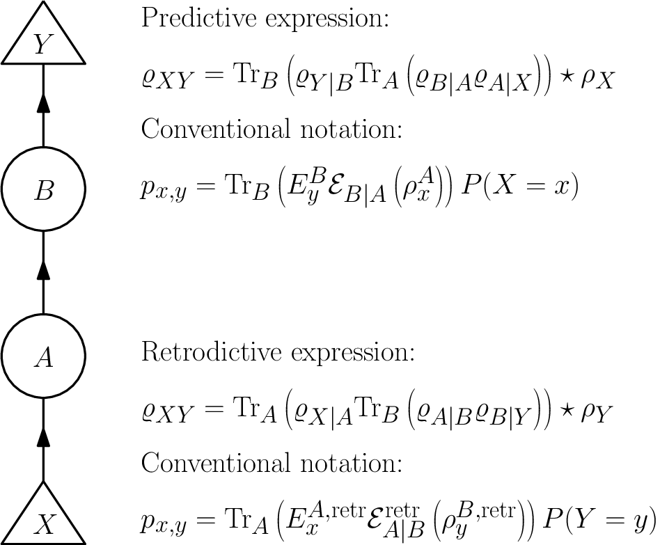
Similarly, the retrodictive expression is obtained from eq (118) by substituting , where and are obtained from and by Bayes’ theorem. This gives
| (143) |
or in conventional notation
| (144) |
To sum up, the formalism of quantum conditional states shows that, just as in the classical case, the rules of quantum Bayesian inference do not discriminate between prediction and retrodiction. Specifically, the rules are the same regardless of whether the propagation is in the same or the opposite direction to the causal arrows. This reveals an important kind of time-symmetry that is not apparent in the normal quantum formalism. More importantly, it shows that a formalism for quantum Bayesian inference can be found that is blind to at least this aspect of the causal structure.
IV.4 Remote Measurements and Spatial Symmetry
Many of the novel features of quantum theory exhibit themselves in the correlations that can be obtained between local measurements on a pair of acausally-related regions. These include Einstein-Podolsky-Rosen correlations and Bell correlations. Inferences about such measurements can be treated using a formalism that is almost identical to the predictive and retrodictive expressions for prepare-and-measure experiments given above. One simply has to substitute the formula for propagating a causal conditional state across acausally-related regions, eq. (55), for the formula for propagating them across causally-related regions, eq. (52), used above.
For two acausally-related regions, and , it is self evident that there is complete symmetry between propagation from one region to another and back again, i.e. if
| (145) |
then
| (146) |
The two conditional states, and are related by the quantum Bayes’ theorem, so Bayes’ theorem allows the direction of belief propagation to be reversed.
To see this spatial symmetry at work, consider the scenario of measurements being implemented on a pair of acausally-related regions, and , as depicted in fig. 12.

In the conditional states formalism, the region is assigned a joint state , and the measurements on and are represented by causal conditional states and . The joint distribution over outcomes is given by the components of the acausal joint state via
| (147) |
These correlations can alternatively be calculated by propagating beliefs about conditioned on to beliefs about conditioned on , and also by propagating beliefs about conditioned on to beliefs about conditioned on . These representations are analogous to the predictive and retrodictive expressions for prepare-and-measure experiments discussed in the previous section. We shall refer to these as rightward and leftward belief propagation respectively.
It may seem convoluted to calculate via rightward or leftward belief propagation, when eq. (147) already gives a simple expression for it. However, it is important to understand how to propagate beliefs across acausally-related regions in order to deal with the situation in which you obtain new information about one region and wish to make inferences about the other. This is exactly what happens in the analysis of an EPR experiment. This problem is known as quantum steering and will be considered in §V.1.3.
First, consider rightward belief propagation. The aim is to rewrite eq. (147) in terms of , the state of conditioned on the region to its left. For greater symmetry with the prepare-and-measure case, we also use and to describe the left hand wing of the experiment, whilst retaining for the right. Then, we write and note that, by Bayes’ theorem,
| (148) |
Substituting these into eq. (147) gives
| (149) |
Expanding the -products gives
| (150) |
All of the terms can be cancelled by using the fact that they commute with and , and by using the cyclic property of the trace. Then, we have
| (151) | ||||
| (152) | ||||
| (153) |
where we have used the cyclic property of the trace and the fact that commutes with and . Eq. (153) has the same form as the predictive expression for a prepare-and-measure experiment with an intervening channel given in eq. (141), except that, in this case, is acausal. We can also use eq. (55) to define , which represents the effective measurement on region that is made by measuring region . Using this, region can be eliminated from eq. (153) to obtain
| (154) |
This is similar to eq. (116), and, in fact, is mathematically identical to it because is a hybrid conditional state, so its mathematical form does not depend on whether it is acausal or causal. Eq. (154) is a useful form to use when we want to consider the effect of measuring on the remote region , as in quantum steering.
For leftward belief propagation, a similar analysis gives the expressions
| (155) |
which is analogous to eq. (143) and
| (156) |
which is analogous to eq. (118).
As with prediction and retrodiction, there is complete symmetry between leftward and rightward belief propagation, and there is a strong symmetry between causal and acausal belief propagation in general. This represents progress towards a theory of quantum Bayesian inference that is completely independent of causal structure.
V Quantum Bayesian Conditioning
Classically, Bayesian conditioning is used to update probabilities when new data are acquired. Specifically, if you are interested in a variable , and you learn that some correlated variable takes the value , then the theory of Bayesian inference recommends that you should update your probability distribution for from the prior to the posterior 66 6 Strictly speaking, this is only a special case of Bayesian conditioning, which can be formulated more generally for arbitrary events on a sample space rather than just for random variables. We restrict attention to the special case of conditioning one random variable upon another for ease of comparison with quantum theory..
Bayesian conditioning can be viewed as a two-step process. First, the observation that causes you to update your probability distribution for from to , where
| (157) |
Secondly, assuming that the observation of does not cause you to change your conditional probabilities , the new probability distribution for is obtained via belief propagation as
| (158) | ||||
| (159) |
This two step decomposition of conditioning has been emphasized by Richard Jeffrey [35, 36] who showed that whenever an observation causes the value of a random variable to become certain, and that all probabilities conditioned on that random variable are unchanged by the observation, then the change in the probability distribution can be represented as Bayesian conditioning.
The reason for emphasizing this decomposition is that Jeffrey was interested in situations in which an observation does not cause you to believe that some variable takes a precise value. As an example of this, adapted from [37], suppose that is the color of a jellybean, which has possible values ‘red’, ‘green’ and ‘yellow’, and that is the flavor, which has possible values ‘cherry’, ‘strawberry’, ‘lime’ and ‘lemon’. Suppose that initially, your probability distribution for , , assigns a probability to each color, and that your observation consists of viewing the jellybean in the light of a dim candle. This might not be enough for you to become certain about the color of the jellybean, but it may reduce your uncertainty somewhat. For example, you may now think it reasonable to assign a probability distribution that gives probability to and each to and . Assuming that the observation does not cause your conditional probabilities to change, Jeffrey shows that your posterior probability distribution for is obtained by belief propagation via
| (160) |
which is known as Jeffrey conditioning.
Many orthodox Bayesians reject the generalization to Jeffrey conditioning and maintain that the rational way to update probabilities in the light of data is always via Bayesian conditioning, not least because most of the apparatus of Bayesian statistics depends on this. This position can be defended by insisting that the sort of situations described above should really be handled by expanding the sample space to include statements about your perceptions. One can show that Jeffrey conditioning can always be represented as Bayesian conditioning on a larger space in this way. Counter to this, Jeffrey argues that it is not realistic to construct such a space, since you do not actually have precise descriptions of your perceptions. This argument has been eloquently put by Diaconis and Zabell [38]:
For example, suppose we are about to hear one of two recordings of Shakespeare on the radio, to be read by either Olivier or Gielgud, but are unsure of which, and have a prior with mass on Olivier, on Gielgud. After hearing the recording, one might judge it fairly likely, but by no means certain, to be by Olivier. The change in belief takes place by direct recognition of the voice; all the integration of sensory stimuli has already taken place at a subconscious level. To demand a list of objective vocal features that we condition on in order to affect the change would be a logician’s parody of a complex psychological process.
The debate over whether Jeffrey conditioning should be subsumed into Bayesian conditioning is somewhat analogous to a similar argument in quantum theory about whether POVMs should be regarded as fundamental, since they can always be represented by projective measurements on a larger Hilbert space via Naimark extension [39].
In the conditional states formalism, the quantum analogue of Jeffrey conditioning is straightforward. If an observation causes you to change the state you assign to a region from to , and if your conditional state for another region , given (which will either be an acausal state or a causal state ) is unchanged, then your posterior state for is determined by belief propagation via either
| (161) |
or
| (162) |
depending on whether and are acausally or causally-related.
The question of whether there is a quantum analogue of Bayesian conditioning is more subtle, as it depends on whether there is a posterior quantum state for that is analogous to having certainty about the value of a classical variable, i.e. the point measure . Arguably, a pure state could play this role, since it represents the smallest amount of uncertainty that one can have about a quantum region. However, unlike classical point measures, pure states still assign probabilities other than and to fine-grained measurements, e.g. measurements in a complimentary basis, and there are good reasons to believe that, even if they represent maximal knowledge, that knowledge is still incomplete [40].
We will not pursue this question further here, but instead focus on the case of a hybrid region . If the the data is the classical variable (so that one can indeed learn its value) then Bayesian conditioning has a straightforward generalization. Upon learning that , the state of should be updated via
| (163) |
Recall that the general form of a state conditioned on a classical variable is , where is a set of normalized density operators and that is simply our notation for . The elements of this set are called the components of , so we may describe Bayesian conditioning as replacing with one of the components of .
Note that, as in the classical case, conditioning can be viewed as a two-step process, wherein first the state of is updated to the diagonal density operator for the point measure, , and then belief propagation is used to determine the posterior state of , as follows
| (164) | ||||
| (165) | ||||
| (166) |
where we’ve made use of the fact that . Note that this holds regardless of the causal relation between and because a hybrid conditional such as does not distinguish between these causal possibilities.
Recall that the rule for propagating unconditional beliefs about to beliefs about is . In conventional notation, this translates to . Therefore, Bayesian conditioning is a process by which a state is updated to an element within a convex decomposition of .
V.1 Examples of Quantum Bayesian Conditioning
In this section, we consider several examples of Bayesian conditioning, based on the different causal scenarios discussed in §III and §IV. In all these cases, conditioning the state of a quantum region on a classical variable is the correct thing to do in order to update the predictions or retrodictions that can be made about other classical variables correlated with the region. In particular, in §V.1.3, we develop the application to quantum steering, showing that the set of states of a region that can be steered to by making remote measurements can be expressed compactly in terms of conditioning and belief propagation.
V.1.1 Conditioning on a Preparation Variable
Consider again the preparation scenario depicted in fig. 3, wherein a quantum region is prepared in one of a set of states depending on the value of a classical variable with prior probability distribution . This can alternatively be described by a conditional state and a diagonal state . In this case, Bayesian conditioning of on the value of corresponds to updating from the ensemble average state to the particular state corresponding to the value of that actually obtains, which is clearly a reasonable thing to do.
The operational significance of this conditioning becomes apparent by considering a measurement made on region , described by a conditional state . We now have a prepare-and-measure experiment, where we are interested in making a predictive inference about the measurement outcome from knowledge of the preparation variable, as depicted in fig. 13.

Eq. (116) gives the predictive expression for the joint probability distribution for this experiment as
| (167) |
From this, we can compute the marginal probability for as
| (168) |
where is the ensemble average state. The conditional is given by
| (169) |
from which it follows that
| (170) |
The transition from eq. (168) to eq. (170) is just classical Bayesian conditioning of the probability for on the value of . Both expressions are representations of the Born rule in terms of belief propagation, and eq. (170) can be obtained from eq. (168) by replacing with , which is just quantum Bayesian conditioning. Thus, quantum Bayesian conditioning on a preparation variable can be used as an intermediate step in updating the probability distribution for a measurement outcome by classical Bayesian conditioning.
Nothing changes if we consider the slightly more complicated scenario where there is an intermediate channel between the preparation and measurement, as depicted in fig. 11. This is because, as shown in §IV.3, the joint probability is still given by eq. (167), where now describes the effective measurement on that corresponds to the actual measurement made on the later region . By similar reasoning, there could be an arbitrary number of time-steps between the preparation and measurement and conditioning the state of on the preparation variable would still be the correct way to update the Born rule probabilities for .
V.1.2 Conditioning on the Outcome of a Measurement
When conditioning on a measurement outcome, it is important to recall that the conditional states formalism assigns states to regions rather than to persistent systems. Therefore, when we update the state of a region by conditioning on a measurement outcome, the resulting conditionalized state is assigned to the very same region that we started with. This is a different concept from the usual state update rules that occur in the standard quantum formalism, such as the projection postulate. These standard rules apply to persistent systems when we are interested in how the state of a system in a region before the measurement gets mapped to its state in a region after the measurement. Because the updated state belongs to a different region than the initial state, this is not an example of pure conditioning in our framework. Therefore, one should not think that conditioning on a measurement outcome must reproduce the projection postulate. The way in which this kind of state update rule is handled in the conditional states framework is discussed in §V.2.
However, there are several other types of inference for which pure conditioning on a measurement outcome is the correct update rule to use. In particular, conditioning can be used for making retrodictions about classical variables in the past of the region of interest. For instance, in a quantum communication scheme, registering the outcome of a measurement on the output of the channel leads us to infer something about which of a set of classical messages was encoded in the quantum state of the channel’s input. The use of conditioning for this sort of inference is the topic of this section.
Recall the measurement scenario depicted in fig. 4. A measurement with outcomes labelled by the classical variable is implemented upon a quantum region . In the predictive formalism, this experiment is described by an input state and a causal conditional state (describing the measured POVM). To condition on a value of , Bayes’ theorem must be applied to determine , and then the component gets picked out by conditioning. This gives
| (171) |
or in conventional notation
| (172) |
The state represents the state of a region prior to the measurement, given the outcome of the measurement, i.e. it is a retrodictive state. Its operational significance is that it allows one to make inferences about variables involved in the preparation of .
To see this, consider again the prepare-and-measure experiment, where now we are interested in making a retrodictive inference from the measurement outcome to the preparation variable, as depicted in fig. 14.

Recall from §IV.3 that there is complete symmetry between the predictive and retrodictive expressions for a prepare-and-measure experiment under exchange of the preparation variable with the measurement variable . Thus, everything that was said regarding the probability distribution for the measurement outcome in the previous example, applies here to the probability distribution for the preparation variable. In particular, the marginal probability distribution for is
| (173) |
and conditioning this on gives
| (174) |
Both of these expressions are belief propagation representations of the Born rule, with respect to the retrodictive POVM for . Thus, conditioning on the outcome of the measurement can be used as an intermediate step in updating the probability distribution for the preparation variable in light of the measurement outcome. The retrodictive state appearing in the retrodictive Born rule simply gets updated by Bayesian conditioning.
As in the previous example, nothing changes if there are intermediate channels between the preparation and measurement. We can simply use conditional belief propagation to eliminate the additional regions.
V.1.3 Conditioning on the Outcome of a Remote Measurement: Quantum Steering
Finally, consider the case of a measurement made on a region that is acausally-related to a region , as depicted in fig. 8. This experiment is described by an acausal joint state , and a conditional state , corresponding to the POVM measured on . We are interested in how the state of the remote region is updated when we learn the outcome of the measurement made on . The updated state of could then be used to predict the outcome of a measurement made on , corresponding to a causal conditional state . This scenario is depicted in fig. 12. The results of §IV.4 establish that the mathematical description of this experiment is formally equivalent to a prepare-and-measure experiment with an intervening channel, the only difference being that the causal conditional state is replaced by an acausal conditional state . This symmetry is enough to establish that, as in the previous example, conditioning the state of on must be the correct way of updating the Born rule probabilities for .
However, it is worth developing this example in a little more detail, since the “remote collapse” at that occurs upon measuring is at the core of the EPR argument. This has led to a study of the ensembles of states for that can be obtained by measuring , a problem known as quantum steering [41, 42, 43, 23, 33, 44, 45, 46]. The conditional states formalism provides an elegant approach to this problem.
Recall from §IV.4, that the joint probability for and can be computed via leftward belief propagation, which yields eq. (156), i.e.
| (175) |
This formula is obtained by first applying Bayesian inversion to to determine
| (176) |
where is the Born rule probability distribution for the measurement outcome. Then, conditional belief propagation is used to obtain .
Eq. (175) is formally equivalent to the retrodictive expression for a prepare-and-measure experiment, so the rationale for conditioning is exactly the same as in the previous example. Specifically, the marginal probability distribution for is
| (177) |
and conditioning on gives
| (178) |
Thus, conditioning the state of on is an appropriate intermediate step for updating the Born rule probabilities for .
The following proposition summarizes this result and translates it into conventional notation.
Proposition V.1.
Let be the joint state of two acausally-related regions. Suppose that the POVM corresponding to the conditional state is measured on and the outcome is obtained. Then, the state of region should be updated from the prior to , where
| (179) |
, and
| (180) |
Let the components of the conditional state be the elements of the POVM and let be the map that is Jamiołkowski-isomorphic to . Then, the updated state of is
| (181) |
where
| (182) |
In the above analysis, the method used to compute is to first apply Bayes’ theorem to and then apply conditional belief propagation. This is the acausal analogue of performing the calculation in the retrodictive formalism. However, we could equally well apply belief propagation first to obtain
| (183) |
and then apply Bayes’ theorem to obtain
| (184) |
This is the acausal analogue of performing the calculation in the Heisenberg picture, and it is straightforward to check that it gives the same result.
In conventional notation, this amounts to first determining the effective POVM on that is performed when is measured via
| (185) |
and then determining the updated state via
| (186) |
Expressions equivalent to these conventional formulas have appeared previously in [33], the only difference being the appearance of a transpose, due to the use of the Choi isomorphism rather than the Jamiołkowski isomorphism in [33].
We have seen that the remote collapse is an instance of quantum Bayesian conditioning. Within interpretations of quantum theory wherein quantum states are considered to describe reality completely, the change of the state of as a result of a distant measurement upon is sometimes considered to be an instance of action at a distance. Indeed, Einstein criticized the Copenhagen interpretation on exactly these grounds. On the other hand, the analysis above shows clearly that if one views quantum theory as a theory of Bayesian inference, then upon learning the outcome of a measurement on , all that occurs is that one’s beliefs about are updated. No change to the physical state of is required within such an approach. This interpretation is bolstered by the formal equivalence to the case of conditioning a region on the outcome of a subsequent measurement, which does not seem to imply retrocausal influences (although for realist interpretations it has been argued that a imposing a particular symmetry principle does imply retrocausality in this scenario [5, 6]).
Einstein anticipated such an epistemic interpretation of remote collapse in his writing, as is argued in [47]. However, he most likely thought that the probabilities represented by quantum states could be probabilities for the values of physical variables (possibly hidden), and that these could satisfy classical probability theory. However, by virtue of Bell’s theorem [48], such an interpretation of remote collapse is not possible within the standard framework for hidden variable theories. We evade this no-go result here by understanding remote collapse as Bayesian updating within a non-commutative probability theory rather than within classical probability theory. In itself, this does not provide a viable realist interpretation of quantum theory, but it does suggest that an acceptable ontology for quantum theory ought not to include the quantum state. Finally, note that our interpretation of remote steering is broadly in harmony with that of Fuchs [22]. However, the view of quantum theory presented here differs from that of Fuchs in that he views quantum theory as a restriction upon classical probability theory whereas we consider it to be a generalization thereof.
V.2 Why the Projection Postulate is not an Instance of Bayesian Conditioning
Finally in this section, we deal with the elephant in the room — the projection postulate. Some authors have argued that the projection postulate is a quantum analogue of Bayesian conditioning (see e.g. [31, 32]). However, the projection postulate is not an instance of quantum Bayesian conditioning as defined above. In this section, we discuss the relationship between quantum Bayesian conditioning and the projection postulate (and quantum instruments in general) at some length, in order to dispel the misconception that projection is a kind of conditioning. After pointing out the formal differences between the two, we explain the different types of update rule that are associated with a measurement in both classical probability theory and quantum theory, pointing out where conditioning and projection fit into this picture. Then, we explain how, in the conditional states formalism, the projection postulate should be thought of as a composite operation, consisting of belief propagation to a later region followed by Bayesian conditioning. This is broadly in line with the treatment of quantum measurements advocated by Ozawa [49, 50]. Finally, we deal with the possible objection that, although the classical analogue of the projection postulate is not just Bayesian conditioning, it can be thought of as conditioning combined with a simple relabelling of the system variable. This argument does not apply in quantum theory because, unlike in a classical theory, any informative measurement necessarily disturbs the system being measured. Although this is well known, we present a formulation of information-disturbance in terms of conditional states, which makes it clear that no quantum instrument can be thought of as conditioning combined with relabelling. This may be of interest in its own right, as it emphasizes the similarity between information-disturbance and other trade-offs in quantum theory, such as the monogamy of entanglement.
In the conventional formalism, when a projective measurement is made on a system , the Lüders-von Neumann projection postulate says that, upon learning the outcome , the initial state should be updated via
| (187) |
For a general POVM , there is a natural generalization of the projection postulate, given by
| (188) |
This generalization has also been proposed as a quantum analogue of Bayesian conditioning [51, 52].
On the other hand, in §V.1.2 the rule for conditioning a state on the outcome of a measurement was found to be
| (189) |
This is distinct from eq. (188) because the roles of and have been interchanged. Furthermore, eq. (188) is not equivalent to an equation of the form of eq. (189) (even allowing a different POVM to appear therein) because the map , like all quantum instruments, is linear on the set of states on , whereas the map is nonlinear on the state space.
If you are inclined to view the projection postulate as the correct quantum generalization of Bayesian conditioning, then you could take this as evidence against the idea that the conditional states formalism provides an adequate theory of quantum Bayesian inference. We shall therefore go to some length to defend the claim that neither the projection postulate nor any other quantum instrument is an analogue of classical Bayesian conditioning.
Consider the scenario depicted in fig. 15. A quantum system located in region and described by the state is subjected to a measurement with outcomes labelled by , and the system persists after the measurement. At this later time, it is represented by a region which, as always in the present formalism, we distinguish from region , but which is associated with a Hilbert space of the same dimension. As discussed in §III.11, a quantum instrument, , determines how the state of is related to the state of , where is the unnormalized state of obtained when .
Now consider the classical analogue of this scenario, depicted in fig. 15. A classical system described by the variable , and assigned a distribution , is subjected to a (possibly noisy) measurement, resulting in the outcome , which is a random variable that depends on through a conditional probability distribution . The system persists after the measurement, where it is described by a random variable . The value of is presumed to depend probabilistically on , and the nature of this dependence may vary with the outcome . This is captured by a conditional probability , which is the classical analogue of a quantum instrument.


It is useful to distinguish three kinds of update rules that might be considered in this scenario, as defined in fig. 15. To describe the difference between these rules, it is useful to introduce some terminology. A distribution over or is said to be a prior distribution if it is not conditioned on the value of , and it is a posterior distribution if it is conditioned on the value of . The temporal ordering that is implicit in this prior/posterior terminology specifies whether the distribution characterizes the knowledge you have before learning the value of or the knowledge you have after learning the value of . In other words, it refers to the time in your epistemological history, relative to the event of learning . On the other hand, the system’s configuration at the time before the occurrence of the measurement will be called its initial configuration and its configuration at the time after the occurrence of the measurement its final configuration. is the initial configuration and the final. The temporal ordering implicit in this latter distinction refers to the time in the system’s ontological history.
Strictly speaking, Bayesian conditioning is a rule that updates what one knows about one and the same variable upon the acquisition of new information. In other words, it maps a prior distribution about some variable to a posterior distribution for that same variable. Consequently, rule BC1, which maps the prior distribution of the initial configuration of the system to the posterior distribution of the initial configuration of the system, is an instance of Bayesian conditioning (it is analogous to updating a retrodictive state as discussed in §V.1.2). Rule BC2 is also an instance of Bayesian conditioning: it maps the prior distribution of the final configuration of the system to the posterior distribution of the final configuration of the system. However, the rule U is not an instance of Bayesian conditioning because it maps the prior distribution of the initial configuration of the system to the posterior distribution of the final configuration. In other words, if one considers and to be distinct variables, then any map from a distribution over one of them to a distribution over the other cannot be an instance of Bayesian conditioning.
We now return to the quantum scenario, this time using the conditional states formalism and paying attention to the analogy with the classical case. The measurement is associated with the causal conditional state that corresponds to the quantum instrument . In the quantum conditional states formalism, there are analogues of each of the three rules we considered above. These are specified in fig. 15. The rule QBC1 corresponds to updating a retrodictive state, as considered in §V.1.2. The von Neumann-Lüders projection postulate is clearly an instance of rule QU. If one stipulates that quantum Bayesian conditioning is a rule that updates the quantum description of one and the same region upon acquiring new information, i.e. that it maps a prior state for a region to a posterior state for the same region, then QBC1 and QBC2 are instances of quantum Bayesian conditioning, but QU is not.
V.2.1 State-Update Rules as a Combination of Belief Propagation and Bayesian Conditioning
If QU is not an instance of Bayesian conditioning, then what is its status within our framework? We now show that it is a composite of two operations: belief propagation followed by Bayesian conditioning.
First consider the classical analogue. The analogue of the projection postulate (or any state update rule arising from an instrument) is given by rule U: . This can be obtained by combining an instance of belief propagation, namely
| (190) |
followed by the rule BC2: , which is an instance of Bayesian conditioning. It is useful to express both these steps in terms of the quantities that are given in the problem, namely, the conditional and the prior over , . The conditional probability distribution used in eq. (190) is simply the marginal of , i.e. . Meanwhile, the expression for the conditional is , where . Setting gives the Bayesian conditioning step as
| (191) |
The quantum analogue of this is straightforward. Quantum state update rules, such as the projection postulate, are of the form QU: . This is simply a sequential combination of quantum belief propagation
| (192) |
with quantum Bayesian conditioning via QBC2: .
Again, it is useful to express each of these steps in terms of the quantities that are given in the problem: the causal conditional state and the prior . The causal conditional state used in eq. (192) is simply a reduced state of , i.e. . To gain some intuition for this step, we translate it into conventional notation. If the quantum instrument associated with is denoted , then eq. (192) becomes
| (193) |
where
| (194) |
The map is the non-selective update map. It is the appropriate map to apply when you know that the measurement has been performed, but you do not know which outcome occurred. The standard update map, which is appropriate when one also knows the outcome, is the selective update map. The projection postulate and its generalization to POVMs are instances of selective update maps. Applying the non-selective update map is just an instance of quantum belief propagation.
Turning to the Bayesian conditioning step, we have , where . Combining these and setting gives
| (195) |
In conventional notation, this translates into
| (196) |
Given the expression for in eq. (193), we see that QBC2 is simply a transition from your prior about the system output by the measurement, the result of applying the non-selective update map, to your posterior about the system output by the measurement, the result of applying the selective update map and normalizing. That this transition from non-selective to selective updates should be regarded as analogous to Bayesian conditioning has previously been argued by Ozawa [49, 50].
In fact, the rule QBC2 is a particular example of the kind of Bayesian conditioning considered in §V.1.1. Every measurement with output region can be considered to define a preparation of for every outcome (assuming a fixed input state). The set of states prepared is given by the components of , which we can compute from the causal joint state by tracing over and conditioning on . The rule QBC2 is then just Bayesian conditioning on , thought of as a classical preparation variable.
V.2.2 No Information Gain Without Disturbance
We have argued that neither the classical rule U nor the quantum state update rule QU are instances of Bayesian conditioning. However, a skeptic might counter that our argument is an artefact of our insistence that the system before and after the measurement should be given different labels. If the conditional distribution in the belief propagation rule of eq. (190) has the form
| (197) |
where is the Kronecker-delta function, then and are perfectly correlated and consequently has precisely the same functional form as . In this case, one could say that the rule U is effectively just Bayesian conditioning.
If is just a delta function, then we say that the measurement is non-disturbing. Recall that for every that characterizes the outcome probabilities for a measurement, there are many conditionals (i.e. classical instruments) that might characterize its transformative aspect and are consistent with . It is not difficult to see that, among all such conditionals, there is always one for which the measurement is non-disturbing, namely,
| (198) |
Of course, there are also many ways of implementing a measurement of such that it is disturbing. Therefore, whilst the update rule U is not an instance of Bayesian conditioning for every possible implementation of the measurement, there is always at least one implementation such that it is effectively just Bayesian conditioning.
The obvious question to ask at this point is whether it is possible to implement a quantum measurement in a non-disturbing way, such that the associated quantum update rule QU (perhaps the projection postulate, perhaps some other rule) is effectively just quantum Bayesian conditioning. For the measurement to be non-disturbing, the causal conditional state in the belief propagation rule of eq. (192) would have to be of the form
| (199) |
i.e it would need to be the partial transpose of the (unnormalized) maximally entangled state. This corresponds to perfect correlation between and because it is Jamiołkowski-isomorphic to the identity channel. If the belief propagation step in the rule QU were of this form, then would have the same functional form as , and the overall quantum update rule QU would be effectively just Bayesian conditioning.
Of course, we are only interested in the case where the measurement is nontrivial. If the measurement gives no information about , then the posterior is the same as the prior and no real conditioning has occurred. Therefore, we restrict our attention to the case where some information is gained. In the language of conditional states, the only kind of measurement that yields no information about the input state is one associated with a causal conditional state that factorizes, that is, one of the form (recall that, in our notation there is an implicit on the right hand side of this equation). In conventional notation, this corresponds to a POVM of the form , which generates a random outcome from the distribution regardless of the state of . We are interested in nontrivial measurements for which does not factorize in this way.
With these definitions in hand, the answer to our question is a resounding “no” — a quantum state update rule of the form QU can never be effectively just Bayesian conditioning because, unlike the classical case, in quantum theory information gain necessarily implies a disturbance. This prevents any QU rule, such as the projection postulate, from being pure Bayesian conditioning. Whilst this fact is well-known, it is instructive to prove it in the conditional states formalism.
Theorem V.2 (No information gain without disturbance).
Consider a measurement described by an instrument associated with the causal conditional state . It is impossible for this measurement to be both informative about () and non-disturbing ().
The proof is a causal analogue of the monogamy of entanglement (see [3] for related ideas).
Proof.
The operator is the partial transpose over of an acausal conditional state . Combining this with the maximally mixed state gives a valid tripartite acausal state via
| (200) |
where is the dimension of . The condition that the measurement be non-disturbing is equivalent to , which implies that the tripartite state should have a reduced state on that is maximally entangled. Meanwhile, the condition that the measurement be informative is equivalent to , which implies that the reduced state on of should not be a product state. But, by the monogamy of entanglement, any tripartite state for which is maximally entangled must have a product state for its reduced state . Hence, both conditions cannot be satisfied simultaneously. ∎
We end with another, less obvious, disanalogy between the quantum and classical cases that bears on the question of how to interpret the quantum collapse rule in our framework. In the previous section, we showed that the classical update rule U could be decomposed into belief propagation followed by Bayesian conditioning. We could just as well have decomposed it in the opposite order: Bayesian conditioning followed by belief propagation. Specifically, we could first apply BC1: , and then propagate the conditioned state via .
It is natural to ask whether such a reverse-order decomposition is possible in the quantum case. That is, can QU: be decomposed into QBC1: , followed by belief propagation ? Perhaps surprisingly, this cannot be done. The belief propagation would have to have the form . But to compute from we need to move from the left of the conditional to the right while keeping on the right. Classical analogy suggests that this could be done using a conditionalized form of the quantum Bayes’ theorem, i.e. . Unfortunately, in the conditional states formalism, valid equations do not necessarily remain valid when we conditionalize each term (this is discussed further in §VII). In particular, the conditionalized form of the quantum Bayes’ theorem is not valid. Not every intuition from classical Bayesian inference carries over into the conditional states formalism.
VI Related Work
In this section, quantum conditional states are compared to other proposals for quantum generalizations of conditional probability and the conditional states formalism is compared to several recently proposed operational reformulations of quantum theory.
VI.1 Comparison to Other Quantum Generalizations of Conditional Probability
Several quantum generalizations of conditional probability have been proposed in the literature, so it is worth comparing their relative merits to the conditional state formalism developed here.
Firstly, Cerf and Adami have proposed an alternative definition of an acausal conditional state [17, 18, 19] (their definition does not extend to the causal case). For a bipartite state , the Cerf-Adami conditional state is
| (201) |
This proposal has a close connection to the calculus of quantum entropies, since the conditional von Neumann entropy of a state can be succinctly written as
| (202) |
which is analogous to the classical formula for the conditional Shannon entropy
| (203) |
Similar compact formulas hold for other information theoretic quantities, such as the quantum mutual information and conditional mutual information.
In [53], Leifer and Poulin introduced a family of conditional states, again restricted to the acausal case, indexed by a positive integer and given by
| (204) |
This unifies the Cerf-Adami conditional state with the definition used in the present work in the sense that and .
The main concern of [53] was the generalization of graphical models and belief propagation algorithms to quantum theory, and their use in simulating many-body quantum systems and decoding quantum error correction codes. In this context, the and cases are particularly interesting. The case is the natural one to use for simulating many-body systems and it allows for a simple generalization of one direction of the classical Hammersley-Clifford theorem, which characterizes the states on Markov Networks. On the other hand, the case is more useful for decoding quantum error correction codes and, as outlined in the present paper, it extends to the causal case and has close connections to quantum preparations, measurements and dynamics that are lacking for other values of . Given that different applications work better with different definitions of the conditional state, it is probably fair to say that there is no uniquely compelling quantum generalization of conditional probability.
With this in mind, note that Coecke and Spekkens have outlined a broad framework for generalizations of conditional probability within the category theoretic approach to quantum theory [54]. Encouragingly, it is possible to derive generalizations of Bayes’ theorem and conditioning abstractly within this framework, but it is not yet clear what axioms within this framework are sufficient to capture all the important aspects of conditioning.
The final quantum generalization of conditional probability to be considered here is the quantum conditional expectation (see [13] for the original paper and [16, 15, 14] for reviews). This was proposed in the context of quantum probability theory, which is a non-commutative generalization of classical measure-theoretic probability within the framework of operator algebras. As such, it is well-defined for systems with infinite dimensional Hilbert spaces as well as for systems with an infinite number of degrees of freedom, for which there is more than one unitarily inequivalent Hilbert space representation. Also, it describes conditioning on an arbitrary algebra of observables, rather than just on a tensor factor as has been considered here. Importantly for the present work, Rédei has proposed an argument based on quantum conditional expectations purporting to show that quantum theory cannot be understood as a theory of Bayesian inference [55] (see also [56]).
However, quantum conditional expectations have a major flaw that is not shared by the conditional states formalism presented here. Fortunately, the full operator-algebraic machinery is not necessary to make the point; the case of finite dimensional Hilbert spaces and conditioning on a tensor factor suffices. Further details of the general case and how the formalism used below follows from it can be found in [14].
Classically, for a pair of random variables, and , a conditional expectation of given is a positive map from functions of and to functions of that satisfies
| (205) |
for all functions that are independent of . Any such map is explicitly given by
| (206) |
where is a conditional probability distribution.
Starting from a joint state , one can obtain a conditional expectation by plugging the associated conditional probability into eq. (206). The main point of this is that it allows the expectation value of any function to be computed from the marginal probability distribution via
| (207) |
The set of functions on and can be thought of as the dual space to the set of probability distributions on and , where the linear functional associated with is given by
| (208) |
i.e. it is the functional that maps the probability distribution to the expectation value of with respect to . With respect to this identification, a conditional expectation has a dual map that maps the space of probability distributions over to the space of probability distributions over and . This is given by
| (209) |
and is called a state extension because every probability distribution gets mapped to a valid probability distribution on a larger space. In addition, state extensions that are dual to conditional expectations satisfy
| (210) |
for every input distribution .
In the finite dimensional, tensor factor case, the quantum conditional expectation of given is a completely positive77 7 The definition only calls for positivity, but it is a theorem that all quantum conditional expectations are completely positive (see [14]). linear map that acts on the set of observables on and satisfies
| (211) |
for all operators . This is analogous to the condition given in eq. (205). The dual map acts on states and is a state extension, which means that
| (212) |
is a valid state for any state on . In addition, the state extensions that are dual to conditional expectations satisfy
| (213) |
for every state on , which is analogous to eq. (210).
As in the classical case, one would like to associate every joint state with a conditional expectation, such that the dual state extension satisfies
| (214) |
i.e. it should give back the state that you started with when you input the reduced state. The analogous requirement is a key property of classical conditional probability as it is what allows an arbitrary joint state to be broken up into a marginal and a conditional that are independent of one another. Unfortunately, the fact that eq. (213) holds for every input state means that this requirement can only be met for product states, i.e. states of the form . This severely restricts the applicability of quantum conditional expectations for describing the correlations present in quantum states. Indeed, they are incapable of representing any correlations at all. This fact is known in the quantum probability literature (see [14] example 9.6), but here is an elementary proof.
Ironically, the easiest way to show that has to be a product state is to use the conditional states formalism as outlined in this paper. The state extension is Jamiołkowski isomorphic to a causal conditional state , where has the same Hilbert space as and the ′ is just used to distinguish the input and output spaces. Then, eq. (214) can be rewritten as
| (215) |
where is the same state as . Similarly, eq. (213) can be rewritten as
| (216) | ||||
| (217) |
for all , where is the same state as and . Since, eq. (217) has to hold for every input state, has to be Jamiołkowski isomorphic to the identity superoperator, so . Since this is pure, monogamy of entanglement88 8 The monogamy of entanglement is well known for positive operators. The fact that it also applies to locally positive operators follows one of the results of [73], which shows that monogamy applies to more general probabilistic theories, including one in which states are locally positive operators. entails that must be of the form for some operator on . Substituting this into eq. (215) gives
| (218) |
which shows that must be a product state and . Therefore, conditional expectations associated with joint states only exist for product states .
It is unclear why quantum probabilists have not regarded this as a fatal flaw in their definition of quantum conditional expectation. However, despite this problem, quantum conditional expectations are still worthy objects of study as they come up in a variety of contexts. For example, the projection onto the fixed point set of a completely positive map is a quantum conditional expectation. The point is just that the terminology “quantum conditional expectation” is an inaccurate way of describing the way that these maps relate to quantum states.
For comparison, the acausal conditional state defined in the present work can also be described as a map , similar to a state extension, with the crucial difference that is not linear. For a conditional state , the map is defined as
| (219) |
The nonlinearity allows this map to satisfy eqs. (213) and (214) without running into trouble with the monogamy of entanglement. Crucially though, because this map is nonlinear, it does not have a dual map that could be regarded as a conditional expectation. Therefore, the close connection between conditional probabilities and conditional expectations breaks down within this formalism.
Rédei’s argument against a Bayesian interpretation of quantum probabilities is based on a variant of Jeffrey conditioning with respect to a quantum conditional expectation. In the present context, if the state of a region is updated from to , then Rédei asserts that the state for should be updated to , where is a state extension derived from the prior state . He then shows that this update rule fails to satisfy an important stability criterion in the infinite dimensional case. Since his argument is crucially based on the linearity of conditional expectations and their duality with state extensions, it does not apply to the nonlinear maps associated with quantum conditional states. However, since the failure only occurs for infinite dimensional systems, a full refutation will have to wait until the conditional states formalism has been extended beyond the finite dimensional case treated here.
To reiterate, it seems unlikely that there is a unique quantum generalization of conditional probability that has properties analogous to every single property of classical conditional probability that is traditionally regarded as important. For this reason, it is important to keep applications in mind when defining quantum conditionals, rather than working in a formal mathematical vacuum.
VI.2 Operational Formalisms for Quantum Theory
Recent efforts to replace the conventional formalism of quantum theory with a new operational formulation — typically in an effort to provide an axiomatic derivation of quantum theory — have much in common with the work presented here. Particularly cognate to our approach is the work of Hardy [57, 58, 59], the Pavia group [60, 61], Oreshkov et al. [62] and Coecke’s group [63, 64].
The reformulation of quantum theory presented by the Pavia group makes heavy use of the Choi isomorphism between quantum operations and bipartite states, and leverages this to represent quantum operations by operators rather than maps. Mathematically, this is also how we achieve a unification of the treatment of acausally-related and causally-related regions. In particular, our proposition III.7, which specifies how to represent a quantum channel in terms of conditional states, is the counterpart to the expression of the action of a quantum channel in terms of the link product. Note that the Pavia group uses the Choi isomorphism whereas we use the Jamiołkowski-isomorphism. The latter has the advantage of being basis-independent, so that the partial transposes that appear in the link product are absent in our approach.
Hardy’s latest work on reformulating quantum theory, using the duotensor framework [59], also represents quantum operations as operators in much the same way as is done in the quantum combs framework and our own. Furthermore, Hardy’s notion of circuit trace (an example of the causaloid product introduced in [57, 59]) provides a unified way of representing a composition of maps as well as tensor products of system states, which is to say, a unified way of representing correlations between acausally-related and causally-related regions. The motivation for Hardy’s work on the causaloid product is very similar to the motivation for our own, namely, to formulate quantum theory in a manner that is even handed with regard to possible causal structures.
Recent work by Oreshkov, Costa and Brukner [62] also represents correlations between acausally-related and causally-related regions is a uniform manner by appealing to the Choi isomorphism.
One notable way in which we depart from all of these approaches is that we treat classical systems internally to the formalism, on a par with quantum systems, rather than as indices on operators representing preparations and measurements.
Finally, we compare our approach to the categorical approach of Coecke, where much of quantum theory (in particular the non-metrical parts) is reformulated using the mathematical framework of symmetric monoidal categories and the graphical calculus that can be defined for these [63, 64]. Systems are the objects of the category, while quantum states and quantum operations are the morphisms. The isomorphism between bipartite states and operations also features prominently in this approach and arises from having a compact structure in the category. Furthermore, classical systems can be treated internally within this framework. It should also be noted that although Coecke’s categorical framework is typically used to formulate quantum theory as a theory of physical processes, it can also be used to express our formulation of quantum theory as a theory of inference. For inference among acausally related regions, this was done in [54]. An extension of this work to the case of inference among causally-related regions should be instructive.
The mathematics of all of these approaches and our own are quite analogous. It is in the interpretational aspect that the greatest differences are to be found. In the reformulations considered above, quantum theory is given a rather minimalist interpretation – it is viewed as a framework for making predictions about the outcomes of certain measurements given certain preparations. Quantum states — however they are reformulated mathematically — are taken to be representations of preparation procedures, while quantum operations are taken to be representations of transformation procedures. These approaches follow the interpretational tradition of operationalism. By contrast, our work takes quantum states to represent the beliefs of an agent about a spatio-temporal region and takes quantum operations to represent belief propagation; it has an epistemological flavor rather than an operational one. For instance, the notions that we deem to be most promising for making sense of the quantum formalism are those one finds in textbooks on statistics and inductive inference, such as Bayes’ theorem, conditional probabilities, statistical independence, conditional independence, and sufficient statistics and not the notions that are common to the operational approaches, such as measurements, transformations and preparations. In this sense, our approach is more closely aligned in its philosophical starting point with quantum Bayesianism, the view developed by Caves, Fuchs and Schack [65, 66, 22, 67, 68]99 9 Unlike the quantum Bayesians, however, we are not committed to the notion that the beliefs represented by quantum states concern the outcomes of future experiments. Rather, the picture we have in mind is of the quantum state for a region representing beliefs about the physical state of the region, even though we do not yet have a model to propose for the underlying physical states..
The particular merit of our epistemological approach is the strong analogy that it affords between quantum inference and classical probabilistic inference. It makes the conceptual content of various quantum expressions more transparent than they would otherwise be. It also bolsters the view that quantum states ought to be interpreted as states of knowledge.
Our take on how to incorporate causal assumptions into quantum theory also has a rather different starting point than the works described above. The relation we posit between the notions of causation and correlation is most informed by the work on causal networks (also known as Bayesian networks), summarized in the textbooks of Pearl [69] and of Glymour, Scheines and Spirtes [70]. We ultimately hope to generalize this analysis of causality by replacing classical probability theory with quantum theory, understood as a theory of Bayesian inference [53]. If the goal is to develop a formalism for quantum theory that is causally neutral then we argue that the causal network approach holds an advantage over the operational approach. Specifically, the problem with taking experimental operations as a primitive notion is that they already have a notion of causal structure built into them insofar as the output of an operation is causally influenced by the input, but not vice-versa (similarly, if the operation is a measurement, then the outcome is causally influenced by the input but not vice-versa). On the other hand, elementary regions — the primitive notion of the causal network approach — are precisely the sorts of thing that can enter into arbitrary causal relations with one another, whilst not having any intrinsic causal structure themselves.
VII Limitations of the -Product
Using the -product makes the conditional states formalism look very similar to classical probability theory. Often, by replacing probabilities with operators and ordinary products with -products, one can obtain an equation that is valid in the conditional states formalism from one that is valid for classical conditional probabilities. However, because the -product is non-associative and non-commutative, this does not always happen. In this section, the limitations of the -product and the disanalogies between classical conditional probabilities and quantum conditional states are discussed.
VII.1 Conditionalized Equations
In classical probability theory, if one takes a universally valid1010 10 Universal validity means that the equation holds for the joint, marginal, and conditional probability distributions derived from any joint probability distribution , rather than holding only in special cases, e.g. due to symmetries or degeneracies of a particular distribution. equation relating conditional, joint and marginal probability distributions over a set of variables and conditionalizes every term on a disjoint variable , then the equation that results is still universally valid. For example, the equation
| (220) |
generalizes to
| (221) |
where a has been placed on the right of the in each term.
Unfortunately, the analogous property does not hold in the conditional states formalism. For example, for acausal states the analog of eq. (221) would be
| (222) |
Writing this out explicitly, the left hand side is
| (223) |
whereas the right hand side is
| (224) |
Because the -product is non-commutative, the terms involving and cannot be brought together and made to cancel as they would in the classical case. Therefore, counterexamples to this rule can occur when and do not commute. For example, it is straightforward to verify that a generalized W-state of the form
| (225) |
does not satisfy this rule. The calculation is not especially instructive, so it is omitted.
Note that a universally valid equation relating quantum conditional, joint and marginal states is still universally valid if one conditionalizes every term on a classical variable. This follows from the equality of the expressions for the left hand and right hand sides of eq. (222) when is replaced by a classical variable .
VII.2 Limitations of Causal Joint States
In §III.5, a causal joint state was defined as an operator of the form . This representation of two causally-related regions highlights the symmetry with the acausal case, since, up to a partial transpose, it is the same sort of operator that would be used to represent two acausally-related regions. Based on this, the quantum Bayes’ theorem was developed in a way that is formally equivalent for acausally and causally-related regions. For this to work, we only needed causal joint states for two causally-related regions. However, since acausal states are not limited to just two regions, it is natural to ask whether causal joint states can be defined for more than two regions. Unfortunately, the naive generalization does not work for scenarios with mixed causal structure, e.g. two causally-related regions that are both acausally related to a third regions, and it also does not work for multiple time-steps.
In the remainder of this section, these limitations are discussed and a different definition of a causal joint state is suggested, which works more generally, but does not exhibit the symmetry between the acausal and causal scenarios for two regions.
VII.2.1 Mixed Causal Scenarios
If region is in the causal future of region , then they can be assigned a causal joint state . The causal conditional state is Jamiołkowski isomorphic to the dynamical CPT map and is the input state. Now suppose that there is a third region, , that is acausally-related to both and , i.e. we start with a joint state of and and apply to region , whilst doing nothing to , to obtain and in a joint state .
One might think that a joint state of could be defined via . We would like this state to have the correct input and output states as marginals, so, in particular, it should satisfy
| (226) |
Unfortunately, this fails because theorem III.4 implies that
| (227) |
whereas
| (228) |
Because there is no trace over , the cyclic property of the trace cannot be used to equate these two expressions.
In fact, in addition to not having as a reduced state, fails to correctly represent the correlations between the causally-related regions and as well, i.e. .
To see the failure of both these conditions explicitly, consider an example in which , and are all of dimension , the input state is a maximally entangled state, and is the identity superoperator. Then, the output state is , and the causal joint state is .
In this case, explicitly calculating the operator gives
| (229) |
Whilst the reduced state gives the correct input state, is not the output state and is not the causal joint state. In fact, no operator of the form can ever satisfy all three conditions , and simultaneously. This is because is a locally positive operator, and hence it must satisfy the monogamy of entanglement, but requiring all three bipartite reduced states to be maximally entangled would violate monogamy and, in fact, only one of the three conditions can be satisfied. Because of this, we have to move beyond locally positive operators in order to faithfully represent all the correlations.
The validity of eq. (227) suggests that using an ordinary product instead of a -product could be a better way of defining a joint state in this scenario. Indeed, the operator does have all the correct bipartite marginals. For example, in our example of maximally entangled input and identity map dynamics, explicit calculation gives
| (230) |
This violates the monogamy of entanglement, which is allowed because it is not a locally positive operator. In fact, it is not even Hermitian.
Whilst this may turn out to be a useful representation, it has a number of disadvantages compared to the -product. First of all, it is non-unique because the operator gives an equally good account of all the correlations. One could even take combinations of the two operators, such as
| (231) |
which might be useful because it is Hermitian.
Secondly, given an arbitrary operator , it is not clear how to check whether it is of the form without running over all possible input states and checking whether is a valid causal conditional state. In contrast, when using the -product, we know that an operator is of the form iff it is the partial transpose of a valid acausal state on , which is a straightforward condition to check.
Finally, a related issue is that, when using the ordinary product instead of the -product, the set of possible causal joint states depends on the causal direction. For an evolution from to , a causal joint state would be of the form , but for an evolution from to it would be of the form . These define two different sets of operators, so we lose the symmetry that was used to obtain Bayes’ theorem in the causal case.
VII.2.2 Multiple Time-Steps
For three space-like separated regions, a Markovian joint state , where and are conditionally independent given , can always be decomposed via the chain rule into
| (232) |
For three time-like separated regions, the analogue of Markovianity is a two time-step dynamics where the first CPT map is and the second is , i.e. it has no direct dependence on . It is natural to ask whether this situation can be represented by a tripartite causal joint state that can be decomposed in a manner similar to eq. (232).
Suppose that the causal conditional states isomorphic to and are and . If the input state is then the first time-step is represented as
| (233) | ||||
| (234) |
and the second time-step is represented as
| (235) | ||||
| (236) |
It follows that
| (237) | ||||
| (238) |
The question is whether the complete dynamics might also be representable as
| (239) |
which in turn would suggest that might be a good candidate for a tripartite causal joint state.
This fails because the expression is not well defined. To see this, expand the first -product to obtain
| (240) |
The term is not well defined because is not a positive operator, but only locally positive, so it may have negative eigenvalues. Hence, it does not have a unique square root. This could be remedied by adopting a convention for square roots of Hermitian operators, such as demanding that the square root of each negative eigenvalue has positive imaginary part. The resulting tripartite operator would then have the correct reduced states, , and , representing the state of the system at each time-step. However, it is not related to a tripartite state of three acausally-related regions via partial transposes, so the symmetry that motivates the use of the -product representation is lost. This loss of symmetry resonates with previous work showing that tripartite “entanglement in time” is not isomorphic to ordinary tripartite entanglement [2].
As with the evolution of a subsystem, these problems can be remedied by using the ordinary product instead of the -product to represent time evolutions, but it is subject to the same disadvantages that were discussed in that context.
VIII Open Questions
VIII.1 The Quantum Conditionals Problem
Monogamy of entanglement is a key feature that distinguishes classical from quantum information. There is a closely related difference between classical conditional probability distributions and acausal quantum conditional states that deserves further investigation. Classically, if is a probability distribution and , are conditional probability distributions then
| (241) |
is always a valid probability distribution. Furthermore, the distribution so defined has the correct marginal and conditional states in the sense that
| (242) | ||||
| (243) | ||||
| (244) |
whenever the left hand sides are well defined.
In the quantum case, the analogous properties do not hold. Although a tripartite state can always be decomposed as
| (245) |
via the chain rule, one cannot start with an arbitrary reduced state and two arbitrary conditional states, and , and expect there to be a joint state that has these conditional and reduced states.
For example, suppose that and are conditionally independent of , i.e. . Now, suppose that is chosen to have more than one nonzero eigenvalue and is chosen to be maximally entangled, e.g. . This implies that the reduced state is pure and entangled. If, in addition, is chosen to be , then the reduced state should also be pure and entangled. However, monogamy of entanglement says that this is impossible, so these choices of conditional state are not compatible. Determining the full set of constraints on coexistent conditional states for three acausally-related regions would be an interesting problem, as would determining the computational complexity of the -party generalization.
IX Conclusions
The formalism of quantum conditional states presented in this paper provides a step towards a formalism for quantum theory that is independent of causal structure, as a theory of probabilistic inference ought to be, and provides a closer analogy between quantum theory and classical probability theory. There is significant potential to use these results to simplify and generalize existing approaches to problems in quantum information theory. As an example of this, in a companion paper [71] we provide an approach to the problems of compatibility and pooling of quantum states that is based on a principled application of Bayesian conditioning and is a direct generalization of existing approaches to the classical versions of these problems. It seems unlikely that the possibility of this approach would have been noticed within the conventional quantum formalism. However, this is only the beginning and we anticipate applications to quantum estimation theory and to quantum cryptography, such as studying the relationship between cryptography protocols that employ different causal arrangements to achieve the same task. As it stands, the formalism is limited to two disjoint elementary quantum regions and the most pressing problem is to generalize it to arbitrary causal scenarios. This is a topic of ongoing work.
Acknowledgements.
We thank David Poulin for useful discussions about conditional states. M.L. would like to thank UCL Department of Physics and Astronomy for their hospitality. Part of this work was completed whilst M.L. was a postdoctoral fellow at the Institute for Quantum Computing, University of Waterloo, Canada, where he was supported in part by MITACS and ORDCF. M.L. also acknowledges support from The Foundational Questions Institute through the Grant RFP1-06-006. Research at Perimeter Institute is supported by the Government of Canada through Industry Canada and by the Province of Ontario through the Ministry of Economic Development and Innovation.Appendix A Proofs of Theorems
Theorem III.4 (Jamiołkowski Isomorphism).
Let be a linear map and let be a linear operator, where is a Hilbert space of arbitrary dimension. Then, the action of on (tensored with the identity on ) is given by
| (246) |
where is given by
| (247) |
Here, labels a second copy of , is the identity superoperator on , and is an orthonormal basis for .
Furthermore, the operator is an acausal conditional state, i.e. it satisfies definition III.1, if and only if is CPT, where denotes the linear map implementing the partial transpose relative to some basis.
To prove this theorem, it is useful to make use of the connection between the Choi and the Jamiołkowski isomorphisms. The map that is Choi-isomorphic to an operator is given by
| (248) |
where is a canonical maximally entangled state defined with respect to a preferred basis for .
The operator is recovered from the map via
| (249) |
Because
| (250) |
eqs. (249) and (247) differ only by whether one uses the projector onto the maximally entangled state (Choi) or the partial transpose thereof (Jamiołkowski) and the two isomorphic maps to are related by , where is the partial transpose operation with respect to the basis used to define the Choi isomorphism.
Proof of theorem III.4.
Now suppose that is an acausal conditional state, i.e. it is positive and . To show that the Jamiołkowski-isomorphic map composed with a partial transpose, , is trace-preserving, note that is trace-preserving, so it suffices to show that is trace-preserving. This proceeds as follows:
| (253) | ||||
| (254) | ||||
| (255) | ||||
| (256) |
To show that is completely positive, note that it is equal to the Choi-isomorphic map , so it suffices to show that the latter is completely positive. By definition
| (257) |
and this is a positive operator for arbitrary positive , where can have any dimension.
Conversely, suppose is CPT. Then, is also trace preserving, so
| (258) | ||||
| (259) | ||||
| (260) | ||||
| (261) | ||||
| (262) | ||||
| (263) |
Also,
| (264) |
and this is a CPT map acting on a positive operator, so is positive. ∎
Theorem III.11.
Let be a hybrid operator, so that by eq. (40) it can be written as
| (265) |
for some set of operators . Then, satisfies the definition of both an acausal and a causal conditional state for given , iff each of the components is a normalized state on .
Proof.
Suppose has the form of eq. (265) for a set of normalized states . Then it is clearly positive and satisfies because for every . Therefore, is an acausal conditional state. On the other hand, is invariant under partial transpose on , so it is also a causal conditional state.
Conversely, suppose that is an acausal conditional state. This means that it is positive and satisfies . Positivity means that for all . If has the form of eq. (265) then taking gives . By varying over all , this implies that each is a positive operator. To prove that these operators are normalized note that
| (266) |
This is an eigendecomposition of with eigenvalues and if this is the identity operator then each of these eigenvalues must be .
On the other hand, if is a causal conditional state, then its partial transpose over must be positive and satisfy . However, operators of the form of eq. (265) are invariant under partial transpose on , so the same argument applies. ∎
Theorem III.13.
Let be a hybrid operator so that it can be written in the form
| (267) |
for some set of operators . Then, satisfies the definition of both an acausal and a causal conditional state for given iff the components form a POVM on , i.e. each is positive and .
Proof.
Suppose has the form of eq. (267) for a POVM . Then it is clearly positive and satisfies . Therefore, is an acausal conditional state. On the other hand
| (268) |
is also positive because the positive operators remain positive under the transpose. Also, . Therefore, is also a causal conditional state.
Conversely, suppose that is an acausal conditional state. This means that it is positive and satisfies . By the same argument used in the proof of theorem III.11, positivity implies that, if is of the form of eq. (267), then each of the components must be positive. Since , the components must form a POVM.
On the other hand, if is an acausal conditional state then, by the argument just given, its partial transpose over must be of the form of eq. (267) for some POVM . This means that itself can be written as
| (269) |
but since the operators form a POVM whenever is a POVM, is of the required form. ∎
Theorem III.15.
Let , and be linear maps such that . Then, the Jamiołkowski isomorphic operators, , and satisfy
| (270) |
Conversely, if three operators satisfy eq. (270), then the Jamiołkowski isomorphic maps satisfy .
Proof.
By definition, the Jamiołkowski isomorphic operator to is
| (271) | ||||
| (272) |
Applying theorem III.6 to gives
| (273) |
and then applying the same theorem to gives
| (274) |
Since is a dummy label in this expression, it can be changed to and then
| (275) | ||||
| (276) |
For the converse direction, we have
| (277) | ||||
| (278) | ||||
| (279) | ||||
| (280) | ||||
| (281) | ||||
| (282) |
∎
References
- [1] B. de Finetti, Theory of Probability, vol. 1 (Wiley, 1974).
- [2] S. Taylor, S. Cheung, C. Brukner, and V. Vedral, in Proceedings of Quantum Communication, Measurement and Computing (AIP, 2004), vol. 734 of AIP Conference Proceedings, pp. 281–284, eprint eprint arXiv:quant-ph/0402127.
- [3] M. S. Leifer, Phys. Rev. A 74, 042310 (2006), eprint eprint arXiv:quant-ph/0606022.
- [4] M. S. Leifer, in Foundations of Probability and Physics – 4, edited by G. Adenier, C. A. Fuchs, and A. Y. Khrennikov (AIP, 2007), vol. 889 of AIP Conference Proceedings, pp. 172–186, eprint eprint arXiv:quant-ph/0611233.
- [5] P. Evans, H. Price, and K. B. Wharton (2010), to appear in British Jnl. for the Philosophy of Sci., eprint eprint arXiv:1001.5057.
- [6] K. B. Wharton, D. J. Miller, and H. Price, Symmetry 3, 524 (2011), eprint eprint arXiv:1103.2492.
- [7] S. Marcovitch and B. Reznik (2011a), eprint eprint arXiv:1103.2557.
- [8] S. Marcovitch and B. Reznik (2011b), eprint eprint arXiv:1107.2186.
- [9] C. H. Bennett, G. Brassard, and N. D. Mermin, Phys. Rev. Lett. 68, 557 (1992).
- [10] C. H. Bennett and G. Brassard, in Proceedings of the IEEE International Conference on Computers, Systems, and Signal Processing (1984), p. 175.
- [11] A. K. Ekert, Phys. Rev. Lett. 67, 661 (1991).
- [12] P. W. Shor and J. Preskill, Phys. Rev. Lett. 85, 441 (2000), eprint eprint arXiv:quant-ph/0003004.
- [13] H. Umegaki, Kodai Math. Sem. Rep. 14, 59 (1962).
- [14] D. Petz, Quantum Information Theory and Quantum Statistics (Springer, 2008), chap. 9.2 Conditional Expectations, pp. 123–130, Theoretical and Mathematical Physics.
- [15] M. Rédei and S. J. Summers, Stud. Hist. Philos. M. P. 38, 390 (2007).
- [16] D. Petz, in Quantum probability and applications III, edited by L. Accardi and W. Waldenfels (1988), vol. 1303 of Lecture Notes in Mathematics, pp. 251–260.
- [17] N. J. Cerf and C. Adami, Phys. Rev. Lett. 79, 5194 (1997a), eprint eprint arXiv:quant-ph/9512022.
- [18] N. J. Cerf and C. Adami, in New Developments on Fundamental Problems in Quantum Physics, edited by M. Ferrero and A. Merwe (Kluwer, 1997b), vol. 81 of Fundamental Theories of Physics, eprint eprint arXiv:quant-ph/9610005.
- [19] N. J. Cerf and C. Adami, Physica D 120, 62 (1998), eprint eprint arXiv:quant-ph/9605039.
- [20] M. Asorey, A. Kossakowski, G. Marmo, and E. C. G. Sudarshan, Open Syst. Inf. Dyn. 12, 319 (2005), eprint eprint arXiv:quant-ph/0602228.
- [21] Z. Zhang and S. Luo, Phys. Rev. A 75, 032312 (2007).
- [22] C. A. Fuchs, J. Mod. Optic. 50, 987 (2003), eprint subatanitally similar to eprint arXiv:quant-ph/0205039.
- [23] L. P. Hughston, R. Jozsa, and W. K. Wootters, Phys. Lett. A 183, 14 (1993).
- [24] P. Hausladen and W. K. Wootters, J. Mod. Optic. 41, 2385 (1994).
- [25] V. P. Belavkin, Radio Engineering and Electronic Physics 20, 39 (1975a).
- [26] V. P. Belavkin, Stochastics 1, 315 (1975b).
- [27] H. Barnum and E. Knill, J. Math. Phys. 43, 2097 (2002), eprint eprint arXiv:quant-ph/0004088.
- [28] S. M. Barnett, D. T. Pegg, and J. Jeffers, J. Mod. Optic. 47, 1779 (2000).
- [29] D. T. Pegg, S. Barnett, and J. Jeffers, J. Mod. Optic. 49, 913 (2002a), eprint eprint arXiv:quant-ph/0207174.
- [30] D. T. Pegg, S. M. Barnett, and J. Jeffers, Phys. Rev. A 66, 022106 (2002b), eprint arXiv:quant-ph/0208082.
- [31] J. Bub, in The Logico-Algebraic Approach to Quantum Mechanics, edited by C. A. Hooker (Dordrecht: Reidel, 1978), vol. II, pp. 209–226.
- [32] J. Bub, Stud. Hist. Philos. M. P. 38, 232 (2007).
- [33] F. Verstraete, Ph.D. thesis, University of Leuven (2002).
- [34] A. Jamiołkowski, Rep. Math. Phys. 3, 275 (1972).
- [35] R. C. Jeffrey, The Logic of Decision (University of Chicago Press, 1983), 2nd ed.
- [36] R. C. Jeffrey, Subjective Probability: The Real Thing (Cambridge University Press, 2004).
- [37] J. Earman, Bayes or Bust? A Critical Examination of Bayesian Confirmation Theory (MIT Press, 1992), chap. 2, pp. 34–35.
- [38] P. Diaconis and S. L. Zabell, J. Am. Stat. Assoc. 77, 822 (1982).
- [39] M. A. Naimark, Izv. Akad. Nauk SSSR Ser. Mat. 4, 277 (1940).
- [40] R. W. Spekkens, Phys. Rev. A 75, 032110 (2007), eprint eprint arXiv:quant-ph/0401052.
- [41] E. Schrödinger, Proc. Camb. Phil. Soc. 31, 555 (1935).
- [42] E. Schrödinger, Proc. Camb. Phil. Soc. 32, 446 (1936).
- [43] M. Vujičić and F. Herbut, J. Phys. A 21, 2931 (1988).
- [44] H. M. Wiseman, S. J. Jones, and A. C. Doherty, Phys. Rev. Lett. 98, 140402 (2007), eprint eprint arXiv:quant-ph/0612147.
- [45] S. J. Jones, H. M. Wiseman, and A. C. Doherty, Phys. Rev. A 76, 052116 (2007), eprint eprint arXiv:0709.0390.
- [46] F. Herbut, J. Phys. A 42, 085202 (2009), eprint eprint arXiv:0809.1631.
- [47] R. W. Spekkens and N. Harrigan, Found. Phys. 40, 125 (2010), eprint eprint arXiv:0706.2261.
- [48] J. S. Bell, Physics 1, 195 (1964).
- [49] M. Ozawa, in Quantum Communication, Computing and Measurement, edited by O. Hirota, A. S. Holevo, and C. M. Caves (Kluwer/Plenum, 1997), pp. 233–241, eprint eprint arXiv:quant-ph/9705030.
- [50] M. Ozawa, Fortschr. Phys. 46, 615 (1998), eprint eprint arXiv:quant-ph/9711006.
- [51] K. Jacobs, Quantum Inf. Process. 1, 73 (2002), eprint eprint arXiv:quant-ph/0201096.
- [52] K. Jacobs, Phys. Rev. A 72, 044101 (2005), eprint eprint arXiv:quant-ph/0503193.
- [53] M. S. Leifer and D. Poulin, Ann. Phys. 323, 1899 (2008), eprint eprint arXiv:0708.1337.
- [54] B. Coecke and R. W. Spekkens, Synthese (2011), published online first, eprint eprint arXiv:1102.2368.
- [55] M. Rédei, International Studies in the Philosophy of Science 6, 129 (1992).
- [56] G. Valente, Stud. Hist. Philos. M. P. 38, 832 (2007).
- [57] L. Hardy (2005), eprint eprint arXiv:gr-qc/0509120.
- [58] L. Hardy, J. Phys. A 40, 3081 (2007), eprint eprint arXiv:gr-qc/0608043.
- [59] L. Hardy (2011), eprint eprint arXiv:1104.2066.
- [60] G. Chiribella, G. M. D’Ariano, and P. Perinotti, Phys. Rev. A 80, 022339 (2009), eprint eprint arXiv:0904.4483.
- [61] G. Chiribella, G. M. D’Ariano, and P. Perinotti, Phys. Rev. A 84, 012311 (2011), eprint eprint arXiv:1011.6451.
- [62] O. Oreshkov, F. Costa, and C. Brukner (2011), eprint eprint arXiv:1105.4464.
- [63] B. Coecke and E. O. Paquette, in New Structures for Physics, edited by B. Coecke (Springer, 2009), Lecture Notes in Physics, pp. 173–286, eprint eprint arXiv:0905.3010.
- [64] B. Coecke, E. O. Paquette, and D. Pavlovic (2009), to appear in Semantic Techniques for Quantum Computation, I. Mackie and S. Gay (eds.), Cambridge University Press, eprint eprint arXiv:0904.1997.
- [65] C. M. Caves, C. A. Fuchs, and R. Schack, Phys. Rev. A 65, 022305 (2002), eprint eprint arXiv:quant-ph/0106133.
- [66] C. M. Caves, C. A. Fuchs, and R. Schack (2006), eprint eprint arXiv:quant-ph/0608190.
- [67] C. A. Fuchs (2010a), eprint eprint arXiv:1003.5209.
- [68] C. A. Fuchs, Physics in Canada 66, 77 (2010b), eprint eprint arXiv:1003.5182.
- [69] J. Pearl, Causality: Models, Reasoning and Inference (Cambridge University Press, 2009), 2nd ed.
- [70] P. Spirtes, C. Glymour, and R. Scheines, Causation, Prediction, and Search (MIT Press, 2001), 2nd ed.
- [71] M. S. Leifer and R. W. Spekkens (2011), eprint eprint arXiv:1110.1085.
- [72] S. D. Bartlett, T. Rudolph, and R. W. Spekkens (2011), to appear in Phys. Rev. A, eprint eprint arXiv:1111.5057.
- [73] H. Barnum, J. Barrett, M. Leifer, and A. Wilce (2006), eprint eprint arXiv:quant-ph/0611295.