The conservative cascade of kinetic energy in compressible turbulence

Turbulence plays a critical role in essentially all astrophysical systems that involve gas dynamics. For example, interstellar turbulence is believed to be driven on large scales by differential galactic rotation or supernovae explosions and dissipated at the smallest scales by microphysical processes. It is widely believed that energy is transferred from the largest scales down to the dissipation scales through a cascade process. Measurements of interstellar scintillation (ISS) ([1]) caused by scattering in the interstellar medium shows a power-law electron density spectrum with a slope close to Kolmogorov’s $-5/3$ scaling over 5 decades in scale. A composite spectrum combining ISS data with that of differential Faraday rotation angle and gradients in the average electron density also yields a Kolmogorov power-law over at least ten decades in scale, dubbed as “the great power-law in the sky” ([2]). High-resolution simulations of the interstellar medium ([3]) also reveal power-law scaling of spectra and structure functions which are reminiscent of incompressible turbulence (albeit with different slopes). Yet, observations of the interstellar medium suggest that the Mach number of turbulent motions is of order $0.1$ to $10$, such that the flow is often compressible ([4]). Similarly, high-resolution simulations of the intracluster medium (ICM) between galaxies ([5, 6]) reveal Kolmogorov-like spectra of kinetic energy at subsonic and transonic Mach numbers. It is not clear how Kolmogorov’s 1941 phenomenology, which forms the cornerstone for our understanding of incompressible hydrodynamic turbulence, can carry over to such flows which exhibit significant compressibility effects. Several recent studies have addressed the problem of compressible hydrodynamic turbulence numerically (e.g. [7, 3, 8, 9, 10]) and theoretically (e.g. [11, 12, 13]), but a physical description equivalent to that of Kolmogorov’s still eludes us.

The idea of a cascade itself is without physical basis since kinetic energy is not a global invariant of the inviscid dynamics. Compressible flows allow for an exchange between kinetic and internal energy through two mechanisms: viscous dissipation and pressure dilatation. While the former process is localized to the smallest scales just like in incompressible turbulence, the latter is a hallmark of compressibility and can a priori allow for an exchange at any scale through compression and rarefaction. Recently, [14, 15] showed how the assumption that pressure dilatation cospectrum decays fast enough rigorously implies that mean kinetic energy cascades conservatively despite not being an invariant. The assumption entails that the mechanism of pressure dilatation acts primarily at the largest scales and vanishes on average at smaller scales. In this Letter, we shall provide the first empirical evidence in support of this assumption.

The outline of this Letter is as follows. Section 2 describes our numerical simulations and Section 3 presents our coarse-graining method for analyzing nonlinear scale interactions. Section 4 discusses the significance of pressure dilatation cospectrum and the assumption we are testing. Our main results are then described in Section 5 followed by a discussion on the role of shocks in Section 6. The Letter concludes with Section 7.

We analyze data from four numerical simulations of compressible turbulence, summarized in Table 1, by solving the continuity, momentum, and internal energy equations

supplemented with an equation of state (EOS) for the fluid. Here, ${\bf u}$ is velocity, $\rho$ is density, $P$ is pressure, $e=P/[(\gamma-1)\rho]$ is internal energy per unit mass for a heat capacity ratio $\gamma$, and ${\bf F}$ is an external acceleration field stirring the fluid. We carry out two kinds of simulations: runs I and III in which the fluid is isothermal and the flow is constantly driven by a non-zero ${\bf F}$, and runs II and IV in which the fluid is an ideal gas and the turbulence is decaying with ${\bf F}={\mbox{\boldmath$0$}}$ (see Table 1).

The simulation domain is a periodic box ${\mathbb{T}}=[0,2\pi)^{3}$. For isothermal forced runs I and III, we start with a uniform density field $\rho({\bf x},t=0)=1$. The forcing function is adapted from [16] and has the form ${\bf F}({\bf x},t)=\sum_{j=1}^{22}\hat{{\bf F}}({\bf k}_{j})\exp{(i{\bf k}_{j}{\mbox{\boldmath$\cdot$}}{\bf x})}+\mbox{complex conjugate}$. The Fourier amplitude, $\hat{{\bf F}}({\bf k}_{j})$, has a compressive component parallel to ${\bf k}_{j}$ and another solenoidal component perpendicular to ${\bf k}_{j}$. On average, the two components are of equal magnitude. The amplitudes and phases of $\hat{{\bf F}}({\bf k}_{j})$ are random in time. The 22 forced wavevectors, $k_{j}$, are nearly isotropically distributed in the range $2\leq|k_{j}|\leq\sqrt{12}$. The initial conditions for unforced decaying Runs II and IV are taken from the last recorded output of Runs I and III, respectively, after reaching a statistically steady state.

We use the central finite-volume scheme on overlapping cells ([17]) to solve eqs. (1)-(2) in conservative form. Instead of solving internal energy eq. (3), the code solves the equivalent total energy equation. The code can also solve compressible ideal magnetohydrodynamics. Details of the whole algorithm have been documented in [18] and [19]. Our method has been verified to achieve the expected order of accuracy and to have very low numerical dissipation. The high-order, low-dissipation, and divergence-free properties of this method make it an excellent tool for simulating compressible hydrodynamic and magnetohydrodynamic turbulence.

Figure 1 plots spectra of the solenoidal and compressive components of the velocity field from runs III and IV, both of which exhibit putative Kolmogorov-like power-law scaling over wavenumber range $k\in[2,50]$. Here, the velocity field is decomposed as ${\bf u}({\bf x})={\bf u}^{s}({\bf x})+{\bf u}^{c}({\bf x})$, such that ${\bf u}^{s}$ is solenoidal and ${\bf u}^{c}$ is irrotational. Spectra from run III are averaged over times after kinetic energy has reached steady state. Spectra from the decaying case, run IV, are normalized at each time by the value of $\langle|{\bf u}|^{2}\rangle$ at that time. Here, $\langle\dots\rangle$ is a volume average over the domain ${\mathbb{T}}$, $\int_{\mathbb{T}}d^{3}{\bf x}(\dots)$.

The key analysis method we use is a “coarse-graining” or “filtering” approach common in Large Eddy Simulation (LES) literature on turbulence modelling. See for example [20, 21, 22] and references therein. The approach was developed by [23, 24] to analyze nonlinear scale interactions in flow fields. It was further refined and utilized by [25] and extended to magnetohydrodynamic ([27]), geophysical ([26]), and compressible ([14, 28, 15]) flows. The method itself is simple. For any field ${\bf a}({\bf x})$, a “coarse-grained” or (low-pass) filtered field, which contains modes at length-scales $>\ell$, is defined as

where $G({\bf r})$ is a normalized convolution kernel, $\int d^{3}{\bf r}~G({\bf r})=1$. An example of such a kernel is the Gaussian function, $G(r)=\frac{1}{\sqrt{2\pi}}e^{-r^{2}/2}$. Its dilation $G_{\ell}({\bf r})\equiv\ell^{-3}G({\bf r}/\ell)$ has its main support in a ball of radius $\ell$. Operation (4) may be interpreted as a local space average.

From the dynamical equation of field ${\bf a}({\bf x})$, coarse-grained equations can then be written to describe the evolution of $\overline{{\bf a}}_{\ell}({\bf x})$ at every point ${\bf x}$ in space and at any instant of time. Furthermore, the coarse-grained equations describe flow at scales $>\ell$, for arbitrary $\ell$. The approach, therefore, allows for the simultaneous resolution of dynamics both in scale and in space, similar to wavelet analysis, and admits intuitive physical interpretation of various terms in the coarse-grained balance.

Moreover, coarse-grained equations describe the large-scales whose dynamics is coupled to the small-scales through so-called subscale or subgrid terms. These terms depend inherently on the unresolved dynamics which has been filtered out. The approach thus quantifies the coupling between different scales and may be used to extract certain scale-invariant features in the dynamics.

Kinetic and internal energy budgets couple through two mechanisms. The first is viscous dissipation which was proved in [28] to be confined to the smallest scales $\ell\leq\ell_{\mu}$ (the dissipation scale-range). Therefore, large-scale kinetic energy in (9) does not couple to internal energy via viscous dynamics for $\ell\gg\ell_{\mu}$. The second mechanism is pressure dilatation, $-P{\mbox{\boldmath$\nabla$}}{\mbox{\boldmath$\cdot$}}{\bf u}$, which exchanges kinetic and internal energy via compression and rarefaction.

It was shown in [14] that if pressure dilatation co-spectrum, defined as

decays fast enough as a function of wavenumber,

then mean pressure dilatation exchanges mean kinetic and internal energy over a transitional “conversion” scale-range of limited extent. Here, $C$ is a dimensionless constant and $L$ is an integral scale. At smaller scales beyond the conversion range, mean kinetic and internal energy budgets statistically decouple giving rise to an inertial range over which mean kinetic energy undergoes a scale-local conservative cascade. In this Letter, we provide the first empirical evidence in support of assumption (14) in Figure 2 which we shall discuss more below.

The idea behind assumption (14) is straightforward and rests on the convergence of a series or an integral at infinity. In the limit of large Reynolds number, assumption (14) implies that mean large-scale pressure dilatation, $PD(\ell)\equiv-\langle\overline{P}_{\ell}{\mbox{\boldmath$\nabla$}}{\mbox{\boldmath$\cdot$}}\overline{{\bf u}}_{\ell}\rangle$, asymptotes to a finite constant, $\theta\equiv-\langle P{\mbox{\boldmath$\nabla$}}{\mbox{\boldmath$\cdot$}}{\bf u}\rangle$, as $\ell\to 0$. In other words, $PD(\ell)$ acting at scales $>\ell$ converges and becomes independent of $\ell$ at small enough scales:

Note that $PD(\ell)$ in (15) (also shown in Figure 3) is a cumulative quantity representing the contribution from all wavenumbers $k<K=\ell^{-1}$, whereas spectra $E^{PD}(k)$ and $E^{u}(k)$ in Figures 1, 2 are density functions. Convergence of $PD(\ell)$ in (15) expresses the decoupling (in an average sense) between large-scale kinetic and internal balances. Such a decoupling is statistical and does not imply that small scales evolve according to incompressible dynamics. However, while small-scale compression and rarefaction can still take place pointwise, they yield a vanishing contribution to the space-average.

We denote the smallest wavenumber at which such statistical decoupling occurs by $K_{c}$.

Over the ensuing wavenumber-range, $K_{c}<K\ll K_{\mu}$ (where $K_{\mu}=\ell_{\mu}^{-1}$), net pressure dilatation does not play a role. For $\ell=K^{-1}$ over this wavenumber-range, budget (9) of large-scale kinetic energy becomes

in a steady state and after space-averaging. If $\langle\epsilon^{inj}\rangle$ is localized to the largest scales as discussed in [28], then $\langle\Pi_{\ell}+\Lambda_{\ell}\rangle$ will be a constant, independent of scale $\ell$.

A constant SGS flux implies that mean kinetic energy cascades conservatively to smaller scales, despite not being an invariant of the governing dynamics. This was one of the main conclusions in [14]. In particular, kinetic energy can only reach dissipation scales via the SGS flux, $\Pi_{\ell}+\Lambda_{\ell}$, through a scale-local cascade process. We are therefore justified in calling wavenumber-range $K_{c}<K\ll K_{\mu}$ the inertial range of compressible turbulence. The existence of this inertial range in such flows warrants expectations that spectra with power-law scalings should exist and that their observation is evidence of a turbulent cascade process similar (although not necessarily identical) to that in incompressible flows.

We will now present results from our simulations to provide the first empirical evidence in support of assumption (14). Figure 2 shows that $|E^{PD}(k)|$ decays at a rate significantly faster than $k^{-1}$, well in agreement with condition (14). We fitted the measurements with power laws over wavenumber range $k\in[2,50]$. We obtain a scaling of $|E^{PD}(k)|\sim k^{-1.88}$ from run III and $|E^{PD}(k)|\sim k^{-1.61}$ from run IV. The measurements shown from runs III and IV are averaged over 21 and 28 evenly-spaced time snapshots, respectively. The plots of $|E^{PD}(k)|$ from run IV are normalized at each time by the value of $\sum_{k}|E^{PD}(k)|$ at that time. We have verified that results from our $512^{3}$ runs I and II are consistent with those presented.

To further illustrate the main idea of this Letter, we analyzed the SGS flux terms, $\langle\Pi_{\ell}+\Lambda_{\ell}\rangle$, in budget (9). Figure 3 shows that pressure dilatation, $PD(\ell)$, tends to a constant beyond a transitional conversion range. Since $PD(\ell)$ is a cumulative quantity representing the contribution from all wavenumbers $k<K=\ell^{-1}$, its convergence to a constant beyond $K=10$ implies that any smaller scales with $k>10$ give a negligible contribution to pressure dilatation. The SGS kinetic energy flux also becomes approximately constant¹¹ 1 Unlike the cumulative quantity $PD(\ell)$ which represents the contribution from all wavenumbers $k<K=\ell^{-1}$, the SGS flux $\langle\Pi_{\ell}+\Lambda_{\ell}\rangle$ is a hybrid quantity involving both wavenumbers $k<K=\ell^{-1}$ (large-scale terms) and $k>K=\ell^{-1}$ (subgrid terms) as definitions (10),(11) show. beyond this conversion range, implying that kinetic energy is cascading conservatively (without any “leakage” to/from internal energy) until the dissipation range is reached. It is notoriously hard to achieve a constant SGS flux range in limited resolution simulations due to viscous contamination. Even the largest-to-date simulation of incompressible turbulence on a $4096^{3}$ grid by [30] does not exhibit a clear constant flux. However, the plots in Figure 3 suggest that an inertial range over which SGS flux is constant does indeed arise at smaller scales over which $PD(\ell)$ plateaus.

Our results and the physical picture we are advancing might seem counter-intuitive at first. After all, a hallmark of compressible turbulence is the formation of shocks and the generation of sound waves. Such phenomena involve compression and rarefaction at all scales and are not restricted to small wavenumbers.

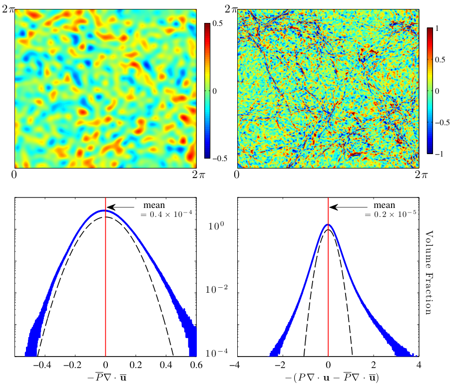
However, there is no contradiction between the existence of such phenomena and our conclusions. Our results concern global pressure dilatation, $-\langle P{\mbox{\boldmath$\nabla$}}{\mbox{\boldmath$\cdot$}}{\bf u}\rangle$, and not the pointwise quantity. While we expect very large pressure dilatation values in the vicinity of small-scale shocks, our results indicate that such a contribution will vanish when averaging over the flow domain due to cancellations between compression and rarefaction regions. For example, linear (small-amplitude) sound waves yield zero mean pressure dilatation, $-\langle P{\mbox{\boldmath$\nabla$}}{\mbox{\boldmath$\cdot$}}{\bf u}\rangle=0$. Figure 4 shows that values of pointwise pressure dilatation at small scales, $-[P{\mbox{\boldmath$\nabla$}}{\mbox{\boldmath$\cdot$}}{\bf u}({\bf x})-\overline{P}_{\ell}{\mbox{\boldmath$\nabla$}}{\mbox{\boldmath$\cdot$}}\overline{{\bf u}}_{\ell}({\bf x})]$, are an order of magnitude more intense relative to large-scale pressure dilatation, $-\overline{P}_{\ell}{\mbox{\boldmath$\nabla$}}{\mbox{\boldmath$\cdot$}}\overline{{\bf u}}_{\ell}({\bf x})$, as expected. The distribution of $-[P{\mbox{\boldmath$\nabla$}}{\mbox{\boldmath$\cdot$}}{\bf u}({\bf x})-\overline{P}_{\ell}{\mbox{\boldmath$\nabla$}}{\mbox{\boldmath$\cdot$}}\overline{{\bf u}}_{\ell}({\bf x})]$ has heavy tails implying spatially rare but intense two-way exchange between kinetic and internal energy. Furthermore, the small-scale distribution has positive skewness implying that conversion from kinetic into internal energy through compression occupies less volume and is more intense relative to conversion from internal into kinetic energy through rarefaction. Despite the larger intensity of conversion at small scales, its global contribution, $-\langle P{\mbox{\boldmath$\nabla$}}{\mbox{\boldmath$\cdot$}}{\bf u}-\overline{P}_{\ell}{\mbox{\boldmath$\nabla$}}{\mbox{\boldmath$\cdot$}}\overline{{\bf u}}_{\ell}\rangle=2.0\times 10^{-6}$, is negligible compared to the mean of large-scale conversion, $PD(\ell)=-\langle\overline{P}_{\ell}{\mbox{\boldmath$\nabla$}}{\mbox{\boldmath$\cdot$}}\overline{{\bf u}}_{\ell}\rangle=3.7\times 10^{-5}$, for $\ell^{-1}=K=20$. This is consistent with the plateau of $PD(\ell)$ in Figure 3.

The origin of such cancellations at small-scales may be understood through the following argument ([14]). While pressure in $-\langle P{\mbox{\boldmath$\nabla$}}{\mbox{\boldmath$\cdot$}}{\bf u}\rangle$ derives most of its contribution from the largest scales, ${\mbox{\boldmath$\nabla$}}{\mbox{\boldmath$\cdot$}}{\bf u}$ is dominated by the smallest scales in the flow. Therefore, pressure varies slowly in space, primarily at scales $\sim L$, while ${\mbox{\boldmath$\nabla$}}{\mbox{\boldmath$\cdot$}}{\bf u}$ varies much more rapidly, primarily at scales $\ell_{\mu}\ll L$, leading to a decorrelation between the two factors. Our numerical results presented in this Letter can be regarded as empirical support to such a physical argument.

The main result of our Letter was to provide the first empirical evidence that pressure dilatation co-spectrum decays at a rate faster than $k^{-1}$, in accord with condition (14). This is sufficient to imply that exchange of kinetic and internal energy through compression and rarefaction takes place at the large scales, on average. At smaller scales beyond a transitional “conversion” scale-range, mean kinetic and internal energy budgets statistically decouple and kinetic energy can only reach dissipation scales via a scale-local conservative cascade process. The existence of such a conservative cascade in compressible turbulence justifies expectations that spectra with power-law scalings should exist in such flows. Furthermore, it suggests that observations of power-law spectra in astrophysical systems are indeed evidence of a turbulent cascade process similar (although not necessarily identical) to that in incompressible flows.

This work leads us to some new questions which we hope to address in future studies. Does the decay rate of pressure dilation cospectrum depend on the decaying/forced nature of the turbulence or on other parameters of the flow such as equation of state, Mach number, and the ratio of compressive-to-solenoidal components of the velocity field? Is the power law scaling of pressure dilation cospectrum that we find in Figure 2 reflecting the asymptotic scaling at arbitrarily high Reynolds numbers? Does the value of $PD(\ell)$ in Figure 3 relative to that of SGS flux increase by increasing the compressive amplitude of the forcing? We invite future studies to investigate these questions and to try and reproduce our results presented in this Letter. Verifying assumption (14) under a variety of controlled conditions would substantiate the idea of statistical decoupling between kinetic and internal energy budgets. This is of paramount importance for future attempts to extend Kolmogorov’s ideas on a conservative cascade of kinetic energy to compressible turbulence.

References

- [1] J. W. Armstrong, J. M. Cordes, and B. J. Rickett. Density power spectrum in the local interstellar medium. Nature, 291:561–564, June 1981.
- [2] J. W. Armstrong, B. J. Rickett, and S. R. Spangler. Electron density power spectrum in the local interstellar medium. Astrophys. J., 443:209–221, April 1995.
- [3] A. G. Kritsuk, M. L. Norman, P. Padoan, and R. Wagner. The Statistics of Supersonic Isothermal Turbulence. ApJ, 665:416–431, August 2007.
- [4] B. G. Elmegreen and J. Scalo. Interstellar Turbulence I: Observations and Processes. Ann. Rev. Astron. Astroph., 42:211–273, September 2004.
- [5] H. Xu, H. Li, D. C. Collins, S. Li, and M. L. Norman. Turbulence and Dynamo in Galaxy Cluster Medium: Implications on the Origin of Cluster Magnetic Fields. Astrophys. J. Lett., 698:L14–L17, June 2009.
- [6] H. Xu, H. Li, D. C. Collins, S. Li, and M. L. Norman. Evolution and Distribution of Magnetic Fields from Active Galactic Nuclei in Galaxy Clusters. I. The Effect of Injection Energy and Redshift. Astrophys. J., 725:2152–2165, December 2010.
- [7] D. H. Porter, P. R. Woodward, and A. Pouquet. Inertial range structures in decaying compressible turbulent flows. Physics of Fluids, 10:237–245, January 1998.
- [8] W. Schmidt, C. Federrath, and R. Klessen. Is the Scaling of Supersonic Turbulence Universal? Phys. Rev. Lett., 101(19):194505, November 2008.
- [9] C. Federrath, J. Roman-Duval, R. S. Klessen, W. Schmidt, and M.-M. Mac Low. Comparing the statistics of interstellar turbulence in simulations and observations. Solenoidal versus compressive turbulence forcing. Astron. Astroph., 512:A81, March 2010.
- [10] M. R. Petersen and D. Livescu. Forcing for statistically stationary compressible isotropic turbulence. Physics of Fluids, 22(11):116101–+, November 2010.
- [11] R. Rubinstein and G. Erlebacher. Transport coefficients in weakly compressible turbulence. Phys. Fluids, 9:3037–3057, October 1997.
- [12] S. Boldyrev. Kolmogorov-Burgers Model for Star-forming Turbulence. Astrophys. J., 569:841–845, April 2002.
- [13] G. Falkovich, I. Fouxon, and Y. Oz. New relations for correlation functions in Navier-Stokes turbulence. Journal of Fluid Mechanics, 644:465, February 2010.
- [14] H. Aluie. Compressible Turbulence: The Cascade and its Locality. Phys. Rev. Lett., 106(17):174502, April 2011.
- [15] H. Aluie. Scale locality and the inertial range in compressible turbulence. J. Fluid Mech. (under review), 2011. arXiv:1101.0150.
- [16] J. Cho and D. Ryu. Characteristic Lengths of Magnetic Field in Magnetohydrodynamic Turbulence. Astrophys. J. Lett., 705:L90–L94, November 2009.
- [17] Y. Liu, C.-W. Shu, E. Tadmor, and M. Zhang. Non-oscillatory hierarchical reconstruction for central and finite-volume schemes. Commun. Comput. Phys., 2:933–963, 2007.
- [18] S. Li. High order central scheme on overlapping cells for magneto-hydrodynamic flows with and without constrained transport method. J. Comput. Phys., 227:7368–7393, 2008.
- [19] S. Li. A fourth-order divergence-free method for MHD flows. J. Comput. Phys., 229:7893–7910, 2010.
- [20] A. Leonard. Energy Cascade in Large-Eddy Simulations of Turbulent Fluid Flows. Adv. Geophys., 18:A237, 1974.
- [21] M. Germano. Turbulence - The filtering approach. J. Fluid Mech., 238:325–336, 1992.
- [22] C. Meneveau and J. Katz. Scale-Invariance and Turbulence Models for Large-Eddy Simulation. Ann. Rev. Fluid Mech., 32:1–32, 2000.
- [23] G. L. Eyink. Local energy flux and the refined similarity hypothesis. J. Stat. Phys., 78:335–351, 1995.
- [24] G. L. Eyink. Locality of turbulent cascades. Physica D, 207:91–116, 2005.
- [25] H. Aluie and G. Eyink. Localness of energy cascade in hydrodynamic turbulence. II. Sharp spectral filter. Phys. Fluids, 21(11):115108, November 2009.
- [26] H. Aluie and S. Kurien. Joint downscale fluxes of energy and potential enstrophy in rotating stratified Boussinesq flows. Europhys. Lett. (under review), 2011. arXiv:1107.5006.
- [27] H. Aluie and G. Eyink. Scale Locality of Magnetohydrodynamic Turbulence. Phys. Rev. Lett., 104(8):081101, February 2010.
- [28] H. Aluie. Scale decomposition in compressible turbulence. Physica D (under review), 2011. arXiv:1012.5877.
- [29] G. Eyink and H. Aluie. Localness of energy cascade in hydrodynamic turbulence. I. Smooth coarse graining. Phys. Fluids, 21(11):115107, November 2009.
- [30] Y. Kaneda, T. Ishihara, M. Yokokawa, K. Itakura, and A. Uno. Energy dissipation rate and energy spectrum in high resolution direct numerical simulations of turbulence in a periodic box. Physics of Fluids, 15:L21–L24, February 2003.