Intermolecular adhesion in conjugated polymers: The role of the band gap and solitonic excitations
Abstract
Conjugated polymers are soft, one-dimensional conductors that admit complex interactions between their polymeric, conformational degrees of freedom and their electronic ones. The presence of extended electronic states along their backbone allows for inter-chain electronic tunneling at points where these polymers make near passes. Using a combination of analytic modeling and Hartree-Fock numerical calculations, we study the localized electronic states that form due to such close encounters between semiconducting conjugated polymers and explore how these states lead to chain–chain binding. We also study the interaction of these inter-chain binding sites with solitonic excitations on the chains. From these results and a modified Poland-Scheraga model, we determine the equilibrium structures of paired-chains formed by intermolecular electronic tunneling. We calculate the energetic ground state of such pairs and show the effective thermal persistence length of the paired chains can vary over an order of magnitude due to the intermolecular binding mechanism.
pacs
82.35.Cd,36.20.Kd,72.80.LeI Introduction
Conjugated polymers [1, 2, 3] can be thought of as soft, low-dimensional conductors or semiconductors. Due to their promise in technological applications such as LEDs, solar cells [4, 5, 6], and even biosensors [7, 8], a great variety of such materials have been synthesized and studied. Independent of their specific chemical details, the existence of extended electronic states along their polymeric backbone provides for their surprising (for a polymer) electronic properties. We refer to these (semi-)conductors as “soft” since their polymeric backbones typically have a short (nanometer scale) thermal persistence length; the conduction path along the polymers in equilibrium solution should be considered to be a tortuous random-walk.
These molecules admit strong correlations between their fluctuating local configurational and electronic properties [9]. In the extreme case, sharp (i.e. localized) bends in the polymeric backbone result in regions of poor electron transport at these so-called conjugation breaks. Conversely, the electronic degrees of freedom of the molecule influence its conformational degrees of freedom. High electronic mobility along the thermally fluctuating backbone’s random path allows for complexities in the interactions of a conjugated polymer with itself and with other such molecules. For example, in conducting chains the pressure of the electron gas trapped between nearby conjugation breaks (sharp bends) in the chain should force such sharp bends apart and thus enhance the statistical weight of locally straighter backbone contours [10]. Thus, the electronic degrees of freedom contribute to the effective persistence length of the polymer. Moreover, looped conformations of the polymer backbone generating close contacts of parts of the polymer separated by a large arc length along its backbone may further perturb the electronic structure of the molecule by introducing tunneling between distant sites along the chain. This sort of “bridge conduction” [11] leads to localized attractive interactions of the polymer at such crossing points where the chain makes a near pass to either itself or another. Based on this electronically mediated intra-molecular attraction, one may imagine that conjugated polymers can self-aggregate into compact globules in solution [11]. At higher polymeric concentrations, one would expect to observe interchain binding, the subject of this article.
More recently, detailed numerical calculations have been preformed that determined the magnitude of these inter-chain tunneling matrix elements for specific conjugated polymers [12]. Using these results and a simple tight-binding model for metallic [13] and/or semiconducting [14] chains, we showed that, for the case of pairs of chains, intermolecular tunneling leads to attractive interactions for which the binding energy is . The tunneling creates a pair of electronic bound states localized at the inter-chain crossing, leading to a total decrease of the electronic contribution to the system’s energy on this scale. One may look at this attractive interaction as an analogue to the traditional covalent chemical bond, but at an energy scale two orders of magnitude weaker. We understand the weakness of the bond to result from a combination of molecular geometry creating a larger than typical internuclear distance in the bond and the energetic cost of localizing the electrons from the extended states of the molecule in order to fill the new localized bound state. The magnitude of this intermolecular, short-ranged interaction suggests that the statistical mechanics of intermolecular binding driven by this mechanism is rather subtle, since both chain configurational entropy and chain bending energies contribute to the free energy of the system at the same energy scale.
In the current article we study in more detail the effect of inter-chain tunneling sites on the electronic states of semiconducting chains by exploring analytically the interaction of pairs of such tunneling sites, the interaction of solitonic chain excitations with such tunneling sites, and determining the electronic ground state of pairs of chains bound uniformly along their length. We also use numerical calculations incorporating more details of the chemical structure of the molecules in question to study the dependence of the electronic binding interaction on the local geometry of the crossing point between the two chains. Finally, we use these results as input to a generalized Poland-Scheraga model describing the binding of two chains. Using this model, we determine the critical concentration for chain pairing and study how the conformational statistics, as parameterized by the effective thermal persistence length of the paired chains evolves as a function of the strength of the binding interaction.
To introduce the bandgap at the Fermi level and thus create the semiconducting state, we use the SSH model [1] for polyacetylene. This simple tight-binding system undergoes a Peierls instability [15]. While this model is based on the specific and uniquely simple model of polyacetylene, we believe that the results we obtain apply more broadly to semiconducting conjugated polymers. Indeed, similar tight-binding models have proven useful in predicting not only the properties of polyacetylene, but have been found to be a useful model for more chemically complex conjugated polymers such as PPV [16, 17]. Thus, we present this model as a general one for the interactions between the electronic degrees of freedom and the conformational state of the polymer.
Our principal results may be summarized as follows. We find (section II.1) that the magnitude of the single-site binding energy and the nature of the bound electron wavefunction are both very similar for the binding metallic or semiconducting chains. This similarity is due to the fact that the binding energy is associated with the creation of localized states having energies far from the Fermi energy, so that the density of states at the Fermi energy in the unperturbed system is not relevant to the inter-chain interaction energy. These results were discussed previously in Ref. [14]. We also examine tunneling site interactions with each other (section II.2) and with solitons that are necessarily present on sufficiently long dimerized chains (section IV). We also compare the lowest-energy bound state configurations of semiconducting and metallic chains. Although these two systems seem similar at the level of individual tunneling sites, in section III we find that the ground states differ rather dramatically [14]. We also discuss the implications of our numerical quantum chemical calculations for the stability of these ground states, determined by the SSH model. In section V we employ these results in the development of a modified Poland-Scheraga model to describe inter-chain binding and the conformational statistics of the result bound chain pairs. We conclude in section VI, and in the Appendices we present the details of our calculations and numerical quantum chemical calculations supporting our binding mechanism.
II Isolated Binding Sites
II.1 A Single Crossing Point
The binding between conjugated polymers is a generic property of the mixing of partially filled -orbitals. We treat the electronic component of the interaction using a simple tight-binding model. To introduce a band gap we use the elegant SSH formalism where a Peierls instability opens a band gap through a distortion of the one dimensional lattice. One could introduce similar tight-binding models with a more complex unit cell appropriate for e.g. PPV [18], but such calculations mask the underlying physics of the system in its most straight forward version. This simplification of the problem has been exploited previously by Guo and collaborators, who showed that the SSH model can be used to study other polymers, such as PPV, with a suitable reinterpretation of the model parameters [19]. Of course, these chemically distinct systems would produce quantitatively different binding interactions, but our primary findings, e.g. that there is an attractive interaction due to the creation of localized states above and below each band, should be generally insensitive to their chemical details. The SSH model also allows us to explore in an analytically tractable manner the interaction between inter-chain binding sites and local lattice distortions such as solitons. These results are also generalizable to other conjugated polymer systems lacking this ground state degeneracy as superpositions of soliton states can be used to model the more general polaron problem in these systems [20].
The SSH Hamiltonian is given by
| (1) | |||||
Here and throughout this article we neglect the dynamics of phonons not associated with the soft phonon mode at the edge of Brillouin zone. We will not consider electron–phonon scattering, but we will allow for more complex static lattice distortions when computing the interaction of tunneling sites and solitons. Here is the tight-binding state at the th site on the chain with spin , is the effective spring constant of the bonds, and is the displacement of the th carbon from its equilibrium position at . Introducing the Peierls instability for the system with one electron per site we generate static lattice distortions (on the scale of ) and shift the hopping matrix elements so that , doubling the unit cell of the lattice. Now the electronic states of the system satisfy the dispersion relation (see Fig. 1a)
| (2) |
which has a total bandwidth of and a bandgap centered around of width [1].
To study the interaction between two chains, we add a second chain with the same Hamiltonian as Eq. 1 and an interaction term of the form
| (3) |
where we have defined the origin to lie at the interaction site, and we have labeled the chains as 1 and 2. The inter-chain hopping parameter implicitly includes the effects of the medium and the relative orientation of the chains. It is also a function of the distance between the linked tight-binding sites with a decay length on the order of a Bohr radius. Quantum chemical calculations on similar conjugated systems have shown that is on the order of 0.1 eV [12]. We assume the chains have adopted a conformation where only one pair of sites is close enough for the inter-chain hopping to be significant. This configuration is illustrated in Fig. 1b and c.


The interaction part of the Hamiltonian given in Eq. 3 can be diagonalized using basis of states that are symmetric or anti-symmetric combinations of the single-chain states,
| (4) |
In this basis the Hamiltonian of the system breaks up into two copies of the single chain Hamiltonian (Eq. 1) that are identical except for the presence of a diagonal element in each sub-space of the Hamiltonian at the interaction site with the value for the symmetric (anti-symmetric) sub-space.
The tunnel matrix element is now analogous to that of an impurity atom in a one dimensional crystal. The impurity potential gives rise to bound states by scattering growing states into decaying states. In appendix A we use a transfer matrix technique to show that the interaction leads to the creation of four bound states as illustrated by the (red) dots in Fig. 1a. Two of these states, termed “ultraband” states [21], appear above the conduction band and below the valance band with energies
| (5) |
while the other two appear in the gap and at the edges of the Brillouin zone with energies
| (6) |
If we assume that we find that, to lowest order, the ultraband states have been shifted away from the band edge by which is unchanged from the metallic case [13]. In contrast, the gap states are shifted by . For half-filled chains, only the two bound states associated with the valence band will be filled. Because the shift of the gap state is smaller than the shift of the ultraband state by for typical parameter values, the result is a net lowering of the energy.
The presence of the binding site will also perturb the energy of the extended electron states. However, as in the metallic case, it can be shown that the total contribution of these states is , where is the total number of tight-binding sites on the polymer, and therefore can be neglected for long chains [13].
In appendix B we present Hartree-Fock (HF) calculations that verify the qualitative features of this binding mechanism. These calculations show that the binding energy is of order and that it is sufficiently insensitive to the precise orientation of the polymers to allow for a variety of aggregate morphologies.
II.2 Two Binding Sites
Since conjugated polymers are semiflexible, it is possible for them to bind in multiple places separated by arc lengths of unbound chains. Two such distant binding sites will experience an effective interaction due to a combination of the change in chain configurational entropy due to the binding constraint, the bending elasticity of the chains, and possibility the electrostatic repulsion of the backbones [22]. In addition, there may be a modification of the binding energy of each binding site due to the interaction of the electronic wavefunctions associated with each of them. We now study this latter effect by determining the shift in total bound state energy of two binding sites as a function of their separation along the chain.
Previously, we demonstrated that the energy shift of an extended state in the presence of a single impurity could be expressed as a series in [13]. Because the symmetric and anti-symmetric states differ only in the sign of the impurity, the odd terms in this series will cancel. Therefore, after summing over the extended states, the total energy contribution from these states must vanish as .
A second binding site introduces a new length , the distance between the binding sites. We expect the perturbation series for the extended states to contain terms proportional to , suggesting that the contribution of the extended states may be non-vanishing for long chains. This is indeed the case. Taking these effects into account, we determine the interaction energy of two binding sites by direct numerical diagonalization of Eqs. 33; the result is shown in Fig. 2. There is an attractive potential well for the two tunneling sites with a minimum at the separation of . At separations greater than about 10 tight binding sites the binding energy is essentially constant, however, at all smaller separations there is a net reduction in energy for even separations and a corresponding increase in energy for odd separations.

This “even-odd” effect can be understood by looking at the states that receive the maximum perturbation from the binding potential. From first order perturbation theory, we expect that the energy shift of a given state to be proportional to the amplitude of that state at the two impurities. Therefore, the states perturbed the most by the two impurities separated by distance will be those with a dominant wavenumber that satisfies the relation . However, the interaction potential induces a phase shift, in the wavefunction. So, the condition for the maximally perturbed state is actually . Because is positive for attractive impurity potentials and negative for repulsive potentials [23], the symmetric states will see the full effect of the impurity potential at smaller values of than the anti-symmetric states.
For the present case of half-filled electronic states, the highest occupied level has a wavenumber . For even we find that so the states with large negative shifts are filled but the corresponding states with large positive shifts are unoccupied. However, if is odd the states with large positive shifts are also filled resulting in an increase in energy relative to the two isolated binding sites. The interaction between two binding sites is discussed in more detail in Appendix C. Given these results, we expect that binding sites should have a weak tendency to cluster so that chains develop finite bound sections in thermal equilibrium. Any conclusions regarding bound-state chain configurations will have to be postponed until we consider the chain configurational entropy of these bound states. We turn to this problem in section V. Before we do so, we consider the problem of multiple inter-chain binding sites (instead of just two) as might occur when the chains adopt a parallel alignment.
III Binding/Non-binding Symmetry
If two chains are aligned in parallel, it is possible to have binding events at every site along the chain as illustrated in Fig. 3. The interaction Hamiltonian is then
| (7) |
This interaction can also be diagonalized using the change of basis shown in Eq. 4. We find that both the valence and conduction bands are split with the chain-symmetrized states dropping in energy by , and the chain-anti-symmetrized ones rising by ; see Fig. 3. For conjugated polymers interacting in solution, however, is considerably smaller than . Thus, the symmetric and anti-symmetric bands have equal occupancy, and there is no net change in energy and no binding.


At first it seems counter-intuitive that the chains can bind at a single site, but have no attraction with many binding sites. To understand this result we now show that there is a symmetry between chains having spatially uniform densities of binding sites and . The lack of binding at maximal tunneling site density is thus understandable since this state is energetically equivalent to no binding sites at all: . This symmetry results in a maximally bound state with interchain tunneling at every other site, i.e. [14].
To observe this proposed symmetry, consider first the Hamiltonian of chains bound at every site: where is the symmetrized/anti-symmetrized non-interacting Hamiltonian, and is the symmetrized version of Eq. 7. As shown in Fig. 3c, this Hamiltonian is identical to apart from equal and opposite constant shifts in the symmetric and anti-symmetric bands. If we now remove the overlap at a single site, we have effectively introduced an (non-binding) impurity site having a potential of strength in the symmetric (anti-symmetric) band. Because of the symmetry in Eqs. 5 and 6, the removal of an interaction at a single site results in the same net energy change as adding a single interaction site to the non-interacting chains. This argument can be extended to any set of interacting sites. Allowing a set of sites to interact on the unbound chains will change the energy of the symmetric band by the same amount as the energy change of the anti-symmetric band upon the removal of interactions from the same set from the fully bound chains. Similarly, the anti-symmetric band on the non-interacting chains changes by the same energy as the symmetric band on the fully bound chains upon the addition/subtraction of interactions at .


The electronic ground state of the pair of parallel chains, as a consequence of this symmetry, requires tunneling at every-other site. The all-trans configuration of the carbon backbone of the polyacetylene molecule as shown in Fig. 4 allows for precisely the required geometry. It is interesting to note that this tunneling site pattern effectively widens the Peierls gap.
More complex conjugated polymers may not be able to achieve this maximally bound state due to e.g. steric interactions of side chains. In spite of the symmetry between pairs of chains having binding density and , we do not expect to observe cases where as a reduction of the number of inter-chain tunneling sites will simultaneously decrease the electronic contribution to the energy of the system and increase the its configurational entropy.
IV Solitons
The dimerization pattern of the tight-binding sites in the SSH model breaks a two-fold symmetry of the system. Reading from the left to the right the slightly longer bond () can either precede or follow the slightly shorter one (). In thermal equilibrium this one-dimensional system cannot maintain long-range order by keeping only one of these two dimerization patterns. One expects to find domain walls where the dimerization pattern switches from to . At the domain wall, or soliton, the pattern of bond lengths is necessarily distorted over some finite distance. These solitonic structures have been studied in detail by Su and collaborators[1]: They found that there are new localized electronic states associated with these domain walls. It remains to be seen how these localized states associated with the solitons are affected by inter-chain tunneling.
For computational simplicity, we first consider the symmetric case in which the two chains each have a single soliton located at the tunneling site. This allows us to separate the binding and anti-binding states using Eq. 4. Furthermore, we simplify the structure of the soliton [1] to that a single-site domain wall. Using our notational short hand, this soliton can be represented as where the filled circle represents both the center of the soliton and the location of the binding site. In Appendix A we show that the bound states associated with this scattering center are given by the solutions of cubic polynomial
| (8) |
In the limit that we find roots corresponding to ultraband bound states at energies , which, except for the term, are identical to the result for metallic chains [13]. We also find another root of Eq. 8 in the gap. This mid-gap state has an energy of . The presence of two solitons has minimal effect on the ultraband bound states, while the mid-gap states associated with the solitons are split by . For half-filled chains the lower gap state is filled for both spin states, while the corresponding upper state remains empty in the electronic ground state of the system. Although solitonic perturbation is linear in , as opposed to the ultraband energy shifts which are , the net energy change is comparable to the binding energy from ultraband states due to the additional factor of . The net result is an enhancement to the binding energy due to the co-localization of the solitons at the inter-chain tunneling site. It is important to note that the binding energy enhancement associated with solitonic co-localization occurs only for uncharged solitons, since charged ones contribute either empty or doubly occupied mid-gap states. The splitting of the filled mid-gap states by the tunneling matrix element results in no net energy change of the system. Now, the energy required to form a soliton is approximately eV [1] suggesting the thermal equilibrium density of uncharged solitons is typically small, but they can also be trapped on long chains by the process of cis- to trans-isomerization; additionally a single uncharged soliton will spontaneously form on chains with an odd number of sites [24, 25]. Thus, soliton co-localization can play a role in the strengthening of isolated inter-chain binding sites, but presumably is less relevant as the number of binding sites increases.
We studied the co-localization of uncharged solitons with the tunneling site numerically in order to explore a more physical extended soliton. Using a profile for the static displacement field of the soliton, we verified the enhancement of the binding energy. The calculation was performed on two chains of 199 sites each with a soliton centered at site 101. We also varied the width of the soliton to ascertain if the presence of the tunneling site altered the minimum energy structure of the soliton as determined by Su and collaborators [1]. We found that such an effect was negligible.
More generally, we determined the change in electronic ground state energy of two chains forming one tunnel junction and each having one soliton whose center is located sites from the tunneling site. Here the index labels the chains. These results are shown in Fig. 5. The principal result is that both solitons are strongly attracted to the the tunneling site, but the strength of the attractive potential of a soliton on one chain is significantly enhanced when the soliton on the other chain is already localized at the tunneling site. This effect results from the mixing of the mid-gap states on each chain due to the inter-chain tunneling matrix element and leads to a further reduction of the energy of the filled mid-gap states. We also note the large amplitude oscillation of the solitonic interaction energy with distance from the tunneling site. This is simply due to the fact that the wavefunction of the mid-gap states has nodes on alternating tight-binding sites.


V Polymer Degrees of Freedom
For polymers in solution, the morphology of their aggregates is determined by the relative strength of the intermolecular binding mechanism and the conformational degrees of freedom of the polymers. These parameters will depend strongly on variables like electrostatic screening and solvent mediation of the interchain hopping parameter. Since these are expected to vary greatly system-by-system, we present a general calculation describing the onset of aggregation.
In sufficiently dilute solution, we expect the formation of stable two-polymer aggregates. These may take the form of loosely-bound, braid-like structures in which the polymers form non-interacting loops between rare binding sites, or zipper-like with the polymers interacting at many consecutive sites [22]. Since the single-site binding mechanism discussed in section II.1 is qualitatively unchanged from the doped case, the braid structures will also be unchanged from conducting polymers discussed earlier [13]. The formation of the tightly-bound, so-called “zipper structures,” however, differs between the conducting and semiconducting polymers. As shown in that previous work on the doped, metallic system, the length of the tightly bound regions is limited by the doping level of the polymers. In the case of undoped, semiconducting polymers, the binding energy due to long, tightly-bound regions grows linearly with their length, provided the binding sites occur at every other site as shown in Fig. 4. For a pair of bound polymers interacting via a series of well-separated tightly-bound regions, the total density of states will be equal to the sum of the density of states for independent segments of tightly bound and free chains weighted by the respective lengths. For this situation (with binding sites at every other site) the dispersion relations for the conduction bands are given by
| (9) |
the valance bands have equal magnitude and opposite signs. We find that the binding energy per site in the tightly bound segments is then given by
| (10) | |||||
| (11) |
where and additional factors of two have been included to account for spin, positive and negative values of , and the fact that two chains are present. This binding energy is the product of the same dimensionful prefactor , found for the single site binding energy, and a dimensionless integral that depends only on the underlying lattice. For parameters typical of polyacetylene this integral generates a factor of , indicating a modest cooperative effect. However, the integral in Eq. 11 is sensitive to the ratio and the cooperativity may be significant in other polymer systems. The transition from single site binding behavior to zipper-like binding occurs when the bound region grows comparable to the localization length .
Without the doping level to limit the length of the zipped region, the amount of chain in the tightly-bound and free states is determined by a competition between the decrease in the system’s total electronic energy and the decrease in the chains’ configurational entropy associated with the binding regions. The statistical mechanics of the binding of two conjugated polymers is thus similar to that of DNA melting [26]. Here we adapt the Poland-Scheraga (PS) model designed for that problem to the current context. There are, however, significant differences between the two systems arising from the difference in bonding mechanism and the lack of unique binding sites on the conjugated polymers, due to the absence of the well-known DNA base pairing mechanism in the system of current interest.
A pair of bound polymers consists of alternating regions of “zipped” (i.e. tightly bound) chains separated by loops of unbound polymer. The partition function for chains of length in such a configuration may be written as
| (12) |
Here and are the Boltzmann weights of the loop and the tightly bound domain respectively, enumerated from the left end of each chain. The number of sites in a tightly bound or “zipped” region, , must be an even number as each chain contributes sites. The size of the loop regions, , are unconstrained because the translational symmetry of the chains allows the formation of asymmetric loops (i.e. the number of sites contributed by chain 1, , is not necessarily equal to the number of sites that chain 2 contributes to the loop, ). The sums over the number of “zipped” and unbound regions and the length of each region are subject to the constraint that the overall lengths of the chains are fixed
| (13) |
The statistical weight of a “zipped” region of bound sites is given by , where accounts for the potentially length-dependent boundary energy between looped and zipped regions, and
| (14) |
is the Boltzmann weight associated with one bound pair of sites (one from each chain) in the “zipped” region. The energy that appears in the exponent has been broken into two parts. The first term is the per site inter-chain binding energy given by Eq. 11 for long tightly bound regions and for a single binding site. In practice we use the form given by Eq. 11 for “zipped” regions of length greater than . Otherwise, we use the result for an isolated binding site. The second term represents a local per-site repulsion between the chains in close proximity. This energy arises from unfavorable steric interactions between the chains enforced by the local binding geometry and possibly electrostatic repulsion between the chains. The details of this energetic term will clearly vary with the chemical details of the specific conjugated polymer system in question. Since is of order , we expect that the net binding energy may be smoothly varied from a minimum of to net repulsive values. The parallel configuration considered below may also contain a van der Waals component enhancing the net attraction [13]. However, this interaction decays much more slowly with distance than interchain hopping, and therefore the details of aggregation on the monomer level will be dominated by the mechanism considered here. We do not consider these details further here.
The transition between a loop and a zipped region of length results in a boundary free energy . This boundary energy has contributions from the cooperativity of the intermolecular bonds, the configurational entropy cost associated with constraining the polymers’ backbone with the formation of the second bond, and a bending energy associated with forming the “Y”-junction where the collinear polymers split into an unbound loop. In the case of conjugated polymers, the first two contributions are negligible due to the weak cooperativity of the bonds and the limited flexibility of the chains. This is in contrast to the situation in nucleic acids where the aromatic base stacking interactions leads to strong cooperativity in the inter-chain bonds while the flexible backbone results in a negligible bending energy and a non-negligible entropic contribution.
For conjugated polymers the statistical weight for the bound regions takes the form
| (15) |
This form accounts for the fact that if the “zipped” region is only a single site long, i.e. a single binding site, the angle between the chains is only weakly constrained. For longer tightly bound regions, however, the chains must be parallel over its length then bend sharply at the start of the surrounding loops. The boundary parameter may be estimated using the conjugation length in a melt. Under these conditions the polymer has conjugation breaks approximately every ten sites [27]. Since there must be two such breaks per tightly bound region and there are four ways of arranging the breaks, the overall Boltzmann weight should be .
The statistical weight for an unbound loop of the paired chains accounts for the configurational entropy of the self-avoiding loop when the loop’s arc length is long compared to the thermal persistence length of the polymer. When the loop is short compared to this length, the bending energy of the chain makes the dominant contribution to the free energy of the loop. These two effects are captured using a weight of the form
| (16) |
with . Here is a length on the order of the persistence length , and we have assumed that short loops trace out the arc of a circle [13]. The constant accounts for the excluded volume of the chains and takes the value in three dimensions [28].
The sums in Eq. 12 are difficult to evaluate because of the restriction imposed by Eq. 13. They can be made more tractable by relaxing this constraint. In order to do so we study the function
| (17) |
which amounts to working in the grand canonical ensemble of the polymer length where we have introduced a fugacity . With the use of Eq. 12 this sum can be rewritten as
| (18) | |||||
where the functions and are defined by
| (19) |
The functions and are defined in analogy to Eqs. 19 and account for the free energy of the tails at the ends of the chain. and will have a different functional form than the portions of chain on the interior of the complex due to the fact that the chain may terminate in either a bound “zipper” or a pair of free tails that are not subject to a loop closure constraint. However, these details are unimportant as the free energy of the system is dominated by the chain interior in the thermodynamic limit.
In the limit of an infinitely long pair of chains i.e. where , the partition function of the two-chain system must scale as , so that the free energy per site is now independent of chain length. The parameter is as yet undetermined, but is related to the free energy per monomer by . From this we recognize the sum shown in Eq. 17 will converge for all . We now determine by examining convergence properties of this sum as given by Eq. 18. Noting that the end effects and necessarily generate bounded corrections, we see that the divergence of the sum will occur at the roots of ; we will ignore all such end effects here and in the following. As we want the dominant term in the limit of long polymers, the free energy is controlled by , the largest root of this equation [29]. From Eqs. 15 and 16, we find that is then given by the solution of
| (20) |
This result allows us to determine the free energy and all thermodynamic properties of the paired chains.
From this result we may compute any number of physically measurable quantities involving the structure of paired conjugated polymers. We will consider three here. First, we compute the fraction of paired chains as a function of polymer concentration in dilute solution, where we will show that, in the limit of sufficiently long polymers, there is a sharp cross-over between free chains and bound pairs as a function of concentration. One may imagine that in the strongly bound limit, more complex bundles of chains should form. Second, we examine the distribution of free loops in the paired chains as a function of the strength of the binding interaction. This result may have measurable consequences for the diamagnetic susceptibility of conjugated polymer solutions. Finally, we compute using a minimal set of assumptions the effective persistence length of the paired chains as a function of the strength of the binding interaction. Such results have implications for the interpretation of scattering data from these polymers in solution.
To calculate the fraction of bound chains we write the free energy for a dilute polymer solution
| (21) | |||||
in terms of the number densities of the unpaired and paired polymers, and respectively. is the total volume of the system. To find the fraction of bound chains as a funtion of the total polymer number density we use the conservation of the number of chains to write and minimize Eq. 21 with respect to . From this we find that
| (22) |
Because of the large polymerization index , the transition from single chains to bound pairs occurs over a very narrow range of binding energies and becomes even sharper as increases [14]. The binding curve is shown in Fig. 6.


The physical properties of bound chains will be determined in part by the statistics of the zipped and loop regions. For example, the magnetic susceptibility of polymeric solution should depend in part on the number density of semiconducting or conducting (for suitably doped chains) loops in solution, which itself will depend on the loop fraction of the individual bound chains. The fraction of zipped regions, which are significantly stiffer mechanically, will determine the effective persistence length of the polymers. We first calculate the distribution of unbound loops.
We consider a pair of bound polymers of length N in the limit so that end effects may be ignored. The partition function for this system is
| (23) |
By translational symmetry all the loops are identical so we calculate the th moment of the length of the first loop from
| (24) | |||||
| (25) |
By the definition of , , so we have
| (26) |
In Fig 7 we plot the average loop size along with its variance. The loops are typically just a few persistence lengths as this length is required to avoid a prohibitive bending energy penalty. The narrow distribution is indicates that longer length loops also incur a prohibitive binding energy penalty.

We now turn to calculation of the effective persistence length of the paired chains. The local bending modulus of the polymer changes markedly when to chains are tightly bound. One should thus be able to distinguish free loops from “zipped” regions of paired chains purely from their local conformational statistics in equilibrium. We first demonstrate this difference in persistence length by estimating its value for free chains and tightly bound ones. In their free state the persistence length of the polymers may be inferred from the conjugation length observed in polymer melts. Given a finite conjugation length of this form, one may simply describe the conformational statistics of the free polymer as a freely rotating chain having a segment length equal to its conjugation length. This length is on the order of ten monomers at for the case of PPV [27], but this value depends on the specific chemical system.
When the chains are tightly bound together in what we call the “zipper” state, the intermolecular bonds will prevent rotations about the polymeric backbone. We imagine the principal remaining source of backbone flexibility on the microscale to come from the bending and stretching of the backbone chemical bonds. The energy scales associated with bond deformation are significantly higher than for the bond rotation of the free chains. The bond stretching modes of the backbone are, in fact, too stiff to play a significant role. Using the estimation of the effective bond-stretching modulus of 21 eV/Å2 we estimate that the effective paired-chain modulus for bending perpendicular to the conjugation plane to be [2]. This is to be compared with the modulus for bending the bonds in the conjugation plane [30]. We estimate that effective persistence length of the paired chain by determining length over which a one radian uniform bend generates one of elastic energy and find that the paired-chain persistence length is at least one order of magnitude bigger than that of the free chain, i.e. .
A representative equilibrium configuration of the paired chains will, in general, consist of a series of alternating “zipped” regions and loops in which the two chains are locally unbound. Since the “zipped” regions are significantly stiffer than the floppy loops, we may approximate the resulting configuration of the paired chains as a random walk consisting of essentially straight “zipped” regions connected by flexible loop regions at which the polymer bends freely. To determine the effective persistence length of the paired chains then we must determine the mean length of the stiffer “zipped” regions in thermal equilibrium. This length is given by the ratio of fraction of bound sites to the fraction of sites that make up the boundary of a “zipped” region: . The latter value is calculated by appending a boundary term to the loop regions such that that counts such boundaries. The fraction of sites that incur this boundary weight is then given by
| (27) |
which may be evaluated by implicitly differentiating Eq. 20. We obtain
| (28) |
The parameter , determining the number of bound sites is given by the derivative
| (29) |
Alternatively, could be calculated from an expression analogous to Eq. 26. The average length of the “zipped” regions is
| (30) | |||||
The various regimes of the effective persistence length can be seen in Fig. 6 as a fraction of the persistence lengths and strength of the binding interaction as parameterized by – see Eq. 14. Based on our calculations, we expect this last parameter to be of order one. In this figure we see that the effective persistence length smoothly crosses over from to as the binding interaction increases for sufficiently long polymers, i.e. for those polymers whose contour length is greater than .
VI Discussion
We have further explored the effect of inter-chain electronic tunneling on polymer pairing (i.e. forming two chain bound states) and on the structure of those pairs in thermal equilibrium. At the level of the formation of an isolated binding site, the binding energy is highly insensitive to the density of states at the Fermi energy of the respective chains. In particular, doped metallic chains, explored earlier [13], and semiconducting ones form individual binding sites that decrease the total electronic energy of the system by . We also investigated the electronic interaction between tunneling sites that are separated by a short arc length along the chain. Here we see that there is a weak attractive interaction between binding sites due to the interaction of the localized states at these tunneling sites. The strength of this attraction is, for at least one physical set of model parameters [12], rather weak, , but this value may vary widely between conjugated polymer systems. The attractive interaction may in some cases lead to the clustering of bound regions.
We support the single tunneling site results of our simple tight-binding model using Hartree-Fock numerical calculations; the numerics also show that the inter-chain binding is somewhat insensitive to the precise orientation of the chains at the tunneling site, although the angle between the chains at the crossing point does lead to significant changes in the binding energy. There we find that the perpendicularly crossed-state which simultaneously allows for the a small separation at the tunneling site and minimizes inter-chain steric repulsion is actually not the lowest energy state. This configuration is a local minimum, while the global minimum occurs for more nearly parallel chains in an orientation consistent with the alternating binding and non-binding sites corresponding to the ground state of the tight-binding model. In the context of that model, we understand the formation of the “every-other” structured ground state in terms of enhancing the Peierls splitting of the conduction and valence bands. It appears from the Hartree-Fock calculations that the local structure of a single binding site also favors the formation of such a “every-other” bound state. It is interesting to note that the crystal structure of polyacetylene shows evidence of this “every-other” bonding pattern [32, 31]. In this case, however, each polymer in the crystal makes contact with several others, but the local equivalence of the pattern of contacts suggests that the electronic mechanisms we consider contribute to the stabilization of this crystal structure.
The binding between two chains is enhanced by the co-localization of solitons with the tunneling sites. The mixing of the mid-gap states associated with the solitons by the tunneling matrix element leads to this binding enhancement for uncharged solitons, but not for charged ones. This effect is weak when there is only one soliton at a tunneling site. Thus, solitonic binding enhancement should scale as the square of the equilibrium (uncharged) soliton density. Recalling that their density in thermal equilibrium is low, we do not expect this to play a large role. It is important to note, however, that a binding event between a charged soliton and an uncharged soliton will result in one of the gap states being half filled and therefore lead to half of the total possible binding enhancement. The density of charged solitons is easily controlled by doping. Using this, one could, in the presence of a sufficient density of charged solitons, produce a significant solitonic enhancement (on the order of per site) of the chain binding energy that scales linearly with the density of uncharged solitons. We expect the same behavior to be observable in polaron/tunneling site interactions in conjugated polymers more chemically complex than polyacetylene.
The statistical mechanics of two paired conjugated polymers is rather subtle since the binding sites generate free energy changes of only per site and allow for significant local conformational freedom at a binding site. The structure of the paired chains results from a nearly equal competition of chain configuration entropy and binding energy. Of course, many of the same subtleties have been addressed in the problem of DNA melting. The one main difference between DNA melting and the binding of conjugated polymers, is that in the latter there is no equivalent of the base-pairing mechanism that promotes the binding in registry of complementary strands. The lack of pairing registry in the current problem enhances the entropic gain of loop-formation by allowing loops of a fixed length to be created from various lengths and (such that ) from the two chains. Using a modified Poland-Scheraga model which accounts for this difference, we found that the effective persistence length varies over at least an order of magnitude as a result of inter-chain binding. The bound regions are significantly stiffer than the unpaired or free loops of the chains allowing us to calculate the effective persistence length of the paired chain in terms of the mean length of the stiff, bound or “zipped” regions.
A number of open questions remain. The spectroscopic signature of the pairing mechanism on two chains is still unresolved. Moreover, the formation of polymeric aggregates of more than two chains remains an open question, particularly with regard to the formation of crystals of conjugated polymers. The fundamental tight-binding approach to the electronic degrees of freedom coupled to the statistical mechanics of the chains, further developed in this article, should provide the basis for these future investigations.
Acknowledgements.
The authors would like to thank F. Pincus, G. Bazan, and A.J. Heeger for stimulating conversations. JDS would also like to thank D. Scalapino and L. Balents for helpful discussions. JDS acknowledges the hospitality of the University of Massachusetts, Amherst. This work was supported in part by the MRSEC Program of NSF DMR00-80034 and NSF DMR02-03755.Appendix A Transfer Matrix Calculations
The one dimensional character of the electronic hopping mechanism lends itself naturally to a transfer matrix approach. In this appendix we review the formalism as it is used to solve for the electronic eigenstates of interacting polymers. In the unperturbed state the eigenstates are normal Bloch waves. The introduction of the inter-chain interaction will scatter these waves and lead to localized states. We begin from the electronic part of the interacting Hamiltonian, Eqs. 1 and 3, and work in the basis of chain symmetrized states as shown in Eq. 4. After this transformation, the symmetric and anti-symmetric parts of the Hamiltonian may be written
| (31) | |||||
where in the symmetric (anti-symmetric) sub-space.
We solve for the energy eigenvalues and the eigenvectors that satisfy the Schrodinger equation . By operating on the Schrodinger equation with the vector we find that the amplitudes obey the set of simultaneous equations
| (32) |
which, along with a trivial identity, may be written in matrix form.
| (33) |
From Eq. 31 the on-site energies vanish everywhere except at the binding site, .
To bring the Hamiltonian into Bloch form, we construct the transfer matrix for a unit cell
| (34) |
If we number the carbons according to 1=2–3=4–5…, where the single and double lines represent long and short bonds respectively, Eq. 34 propagates of the wavefunction between consecutive odd sites. As required by the discrete translational invariance of the Hamiltonian, Eq. 34 takes a diagonal form in the momentum basis
| (35) |
where is the unit cell dimension of the dimerized chain, and
| (36) | |||||
The first of these equations implicitly redetermines the dispersion relation of the Bloch waves making up the energy eigenstates of the system. The solution is given below in Eq. 41. For completeness we also report the change of basis matrix defined by Eq. 35 in terms of the dimensionless parameter given by
| (40) |
The complex number is the phase change of the wavefunction associated with the quantum number (wavenumber) across the long bonds separating one unit cell from the next. In other words: , as may be checked using Eqs. 33, 34, and 40. The phase shift within a unit cell is so that the total phase shift from one unit cell to the next is , as required by Bloch’s theorem.
Of course, the condition for bounded eigenfunctions is that must be real, leading to the dispersion relation
| (41) |
which has a total bandwidth of and a bandgap centered around of width .
To study the effect of the binding site on the electronic spectrum we repeat the transformation Eq. 35 with the dimer containing the binding site at . The result is
| (42) |
where . In addition to the states given by Eq. 2 for , the off-diagonal elements in Eq. 42 allow normalizable states with complex wavenumber through the scattering of a growing wave into a decaying one. This is accomplished when the upper left matrix element vanishes, therefore
| (43) | |||||
| (44) | |||||
| (45) |
With a little more algebra we find that the four bound states shown in Fig. 1c are given by
| (46) |
where the upper sign applies to the “ultraband” states (Eq. 5) and the lower sign applies to the gap states (Eq. 6) [21].
We now compute the analogous bound state associated with a tunneling site localized at the center of an idealized soliton. We represent the soliton as a single-site disruption of the dimerization pattern as discussed in Section IV. It may be written as: and has undistorted unit cells on either side of the soliton’s center () connected to that special site by the long bonds () that have tunneling matrix element . The tunnel matrix element also occurs at this special and central site.
The transfer matrix at the central site is
| (47) |
Upon changing basis as shown in Eq. 35 we find
| (48) | |||
Once again, the bound states exist for values of where the upper left element vanishes, so we have
| (52) |
| (53) |
The solutions are given by the roots of the polynomial
| (54) |
It is easily verified that the solution does not satisfy Eq. 52, and thus we arrive at Eq. 8.
Appendix B Hartree-Fock Calculations
To better understand the limitations of the tight-binding model and explore the role of steric interactions near the tunneling site for the specific case of polyacetylene we numerically computed the binding energies of two short (20 monomers each) polyacetylene oligomers with quantum chemical calculations using the package Gaussian [33]. After relaxing a single chain of fixed length, we introduced an identical chain in various geometries. In each case the interaction energy was calculated as the energy of the two chain system minus twice the energy of the single chain. Energies were evaluated using the non-counterpoised Hartree-Fock technique with the 6-31G* basis set. Additional calculations using the B3LYP method found results qualitatively similar to those from Hartree-Fock (data not shown).


Using this procedure we tested the distance and orientation dependence of the binding energy due to a single tunneling site. We parameterized the geometry of the near miss of two chains by two angles and one distance. As shown in Fig. 8, the perpendicular distance between the two chains at the binding site is . The angle measures the rotation of the plane containing the intra-chain carbon bonds of one polymer about an axes parallel to that chain. Finally, the angle between the long axes of the two chains (looking down along the direction parallel to the vertical displacement ) is given by . In Fig. 9 we show the binding energy obtained numerically as a function of and for a fixed value of (i.e. with the conjugation planes parallel). As expected for the tunneling mechanism, the attractive interaction decays rapidly (exponentially) with distance reaching minimum at Å for all values of .

The angular dependence at fixed is more complex. For Å corresponding to maximum binding, the attractive interaction has a minimum at the perpendicular crossing of the chains () where the net binding energy is eV. This local minimum is globally unstable; there are deeper minima near corresponding to more nearly parallel alignments of the chains. The minimum is deepest and in closer agreement to the “every other” site ground state predicted by the tight binding model. For precisely parallel alignments () in which the chains are stacked on top of each other as shown in Fig. 3, they do not attract, as predicted by our tight binding model. In fact, interactions not included in our model give a repulsive interaction of eV. Our results are consistent with previous work that has shown the maximally overlapped configuration to be a high energy state with more favorable interactions occurring when one of the molecules is rotated or translated such that the overlap is removed from some of the carbons [34, 35].
The binding energy shown in Fig. 9 is also insensitive to the precise lateral alignment of the two chains at the binding site. We shifted the top chain by Å in the positive and negative X and Y directions, where lies along the Z direction. These shifts altered the binding energy by less than 6%. These data are not shown.
Finally, we rotated the upper chain by the angle as defined in Fig. 8. This rotation preserved the Å separation between the two carbons at the binding site. For negative rotations the interaction becomes less favorable due to the steric repulsion of the nearby carbons of the two chains, but for positive rotations the binding energy increases to eV at an angle of , as shown in Fig. 10. Note that these energy shifts are significantly less than suggesting that the rotational motion of the polymers is unconstrained by the tunneling sites in thermal equilibrium.

We find that these results are only weakly dependent upon chain length; for example, as the chain lengths were increased from ten to forty carbons, the depth of the well increased by about five percent. In order for the numerically obtained binding energies to match our tight binding results, we need to set eV and eV. This result is consistent with the overlap measured in Ref. [12] for configurations where the contact extends over the entire molecule.
The Hartree-Fock calculations presented here support the notion of intermolecular bonds forming at the close approach of two polyacetylene chains. The strength of these interactions is consistent with previous studies [12]. The range of the attraction is as expected for the proposed tunneling mechanism and its angular () dependence suggests both perpendicular and nearly parallel arrangements are favored for a single binding site. The binding interaction, however, is sufficiently insensitive to the precise orientation of the polymers as to allow the polymers to form a variety of aggregates.
We conclude by noting that the ab initio calculation of the interactions between -conjugated molecules is an area of ongoing research [34, 36]. While significant advances have been made for small aromatic molecules, these molecules lack the extended orbitals essential to our model. These methods are not feasible for the larger systems we require, and therefore, we have employed the significantly less accurate HF method. While we are encouraged by the qualitative agreement with our tight-binding model, we emphasize that our HF results should not be viewed as quantitative.
Appendix C Binding Site Interactions
To examine the interaction energy between two tunneling sites we consider a chain of tight binding sites. We place the two tunneling sites, which act like impurity potentials, at sites and such that the the tunneling sites are symmetrically placed about the center of the chain: . This provides a computational convenience without greatly reducing the validity of the results so obtained. The position of the localized states along the chain should be irrelevant on long polymers provided neither tunneling site is within its localization length (a few lattice constants) of the chain ends.
Since the even-odd effect observed in Fig. 2 is unchanged by the chain dimerization, we consider the case of a uniform chain with and dispersion . The eigenstates have the form
| (55) | |||||
where is an amplitude to be determined, and the sign of the final term is determined by parity. The boundary conditions require that the wavefunction be an eigenstate of the parity operator and and remain continuous at the impurities so that
| (56) | |||
| (57) |
We derive a final condition by requiring that the Schrödinger equation is satisfied at the impurity sites
| (59) |
Using Eqs. 56, 57, and 59 we find the conditions on for states of even and odd parity are
| (60) | |||||
| (61) |
We would like to examine the change in energy of the states as the distance between the impurity potential is changed but the length of the chain is constant. To do this we make the substitution and find that the quantization conditions become
| (62) | |||||
| (63) |
To see the energy shift of the individual states it is helpful to graphically solve these equations. In Fig. 11 we plot both sides of Eq. 62 for the symmetric and antisymmetric states () and . The left side of the equation, drawn in dashed lines, is a series of tangent curves with a spacing set by the length of the chain. For very long chains these tangent curves will be spaced infinitesimally close together. The allowed values are found at the intersections of the solid curves and the dashed curves. In the limit , the solid curves lie along the axis and we find the unperturbed states satisfy where is an integer. For small positive values of the right side of the equation takes positive values and the eigenstate is shifted to larger values. Similarly, negative values of shift the states to longer wavelengths. Therefore, the amplitude of the solid curves in Fig. 11 grows with the magnitude of the wavenumber shift of the eigenstates.
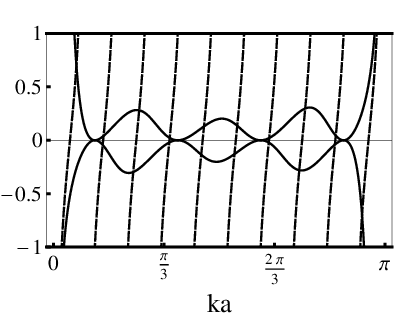
We see in Fig. 11 that, although the curves for positive and negative values of oscillate with the same period, the curves are not symmetric about the axis. Starting at small , there are alternating regions where the symmetric states are shifted more than the anti-symmetric states and vice versa. The origin of this asymmetry between the sub-spaces is the phase shift induced by the impurity potentials discussed in section II.2. The contribution of these states to the total energy of the system will depend on the location of the Fermi level. If the separation between the binding sites, , is even the Fermi level, , lies just above a region of large shift for the symmetric states and below the corresponding region of large shifts for the anti-symmetric states. This results in a net negative contribution to the binding energy. However, if the separation is odd the Fermi level lies immediately above a region of large shifts for the anti-symmetric states and the contribution is positive.
References
- [1] W.P. Su, J.R. Schrieffer, and A.J. Heeger, Phys. Rev. Lett., 42, 1698 (1979).
- [2] W.P. Su, J.R. Schrieffer, and A.J. Heeger, Phys. Rev. B, 22, 2099 (1980).
- [3] H. Takayama, Y.R. Lin-Liu, and K. Maki, Phys. Rev. B, 21, 2388 (1980).
- [4] A.J. Heeger and M.A. Diaz-Garcia Curr. Opin. Sold State Mater. Sci., 3, 16 (1998).
- [5] G. Yu, J. Gao, J.C. Hummelen, F. Wudl, A.J. Heeger Science 270, 1789 (1995).
- [6] G. Yu, J. Gao, J. Hummelen, F. Wudl, and A.J. Heeger, Science 270, 1789 (1995).
- [7] L.H. Chen, D.W. McBranch, H.L. Wang, R. Helgeson, F. Wudl, and D.G. Whitten, Proc. Natl. Acad. Sci. (USA), 96, 12287 (1999).
- [8] B.S. Gaylord, A.J. Heeger, and G.C. Bazan, Proc. Natl. Acad. Sci. (USA), 99, 10954 (2002).
- [9] D.W. Hone, P.A. Pincus, C. Singh, and G. Rossi Synth. Met. 41-43, 3419 (1991).
- [10] P.A. Pincus, G. Rossi, and M.E. Cates Europhys. Lett. 4, 41 (1987).
- [11] D.W. Hone and H. Orland Europhys. Lett. 55, 59 (2001).
- [12] J.L. Brédas, J.P. Calbert, D.A. da Silva Filho, and J. Cornil, Proc. Natl. Acad. Sci. 99, 5804 (2002).
- [13] J.D. Schmit and A.J. Levine, Phys. Rev. E 71, 051802 (2005).
- [14] J.D. Schmit and A.J. Levine Phys. Rev. Lett. 100, 198303 (2008).
- [15] R. Peierls, Quantum Theory of Solids, Clarendon Press, Oxford (1955).
- [16] J. Fink and G. Leising, Phys. Rev. B 34, 5320 (1986).
- [17] Z.G. Yu, R.T. Fu, C.Q. Wu, X. Sun, and K. Nasu, Phys. Rev. B 52, 4849 (1995).
- [18] N. Kirova, Brazovskii, and A.R. Bishop, Synth. Met. 100, 29 (1999).
- [19] F. Guo, et al. Phys. Rev. Lett. 74, 2086 (1995).
- [20] A. J. Heeger, S. Kivelson, J. R. Schrieffer, and W. -P. Su, Rev. Mod. Phys. 60, 781 (1988).
- [21] S.R. Phillpot, D. Baeriswyl, A.R. Bishop, and P.S. Lomdahl, Phys. Rev. B, 35, 7533 (1987).
- [22] I. Borukhov, R.F. Bruinsma, W.M. Gelbart, and A.J. Liu, Phys. Rev. Lett. 86, 2182 (2001).
- [23] An electronic state scattering off an impurity potential, at the origin has the form . Using the requirements that the wave satisfy the Schrödinger equation and is continuous at the impurity site, we solve for the undetermined amplitude, , and the phase shift .
- [24] W.P. Su, Solid State Comm. 35, 899 (1980).
- [25] W.P. Su and J.R. Schrieffer, Proc. Nat. Acad. Sci. USA 77, 5626 (1980).
- [26] D. Poland and H. A. Scheraga, Theory of Helix-Coil Transistions in Biopolymers, Academic Press, New York (1970).
- [27] S. Heun, R. F. Mahrt, A. Greiner, U. Lemmer, H. Bassler, D. A. Halliday, D. D. C. Bradley, P. L. Burn and A. B. Holmes, J. Phys. Condens. Matter 5, 247 (1993).
- [28] Y. Kafri, D. Mukamel, L. Peliti, Phys. Rev. Lett. 85, 4988 (2000).
- [29] S. Lifson J. Chem. Phys. 40, 3705 (1964).
- [30] M. Canales and G. Sesé, J. Chem. Phys. 118, 4237 (2003).
- [31] H. Kahlert, O. Leitner, and G. Leising, Synth. Met. 17, 467 (1987).
- [32] M. Winokur, Y.B. Moon, A.J. Heeger, J. Barker, D.C. Bott, and H. Shirakawa, Phys. Rev. Lett. 58, 2329 (1987).
- [33] Gaussian 03, Revision B.05, M. J. Frisch, G. W. Trucks, H. B. Schlegel, G. E. Scuseria, M. A. Robb, J. R. Cheeseman, J. A. Montgomery, Jr., T. Vreven, K. N. Kudin, J. C. Burant, J. M. Millam, S. S. Iyengar, J. Tomasi, V. Barone, B. Mennucci, M. Cossi, G. Scalmani, N. Rega, G. A. Petersson, H. Nakatsuji, M. Hada, M. Ehara, K. Toyota, R. Fukuda, J. Hasegawa, M. Ishida, T. Nakajima, Y. Honda, O. Kitao, H. Nakai, M. Klene, X. Li, J. E. Knox, H. P. Hratchian, J. B. Cross, C. Adamo, J. Jaramillo, R. Gomperts, R. E. Stratmann, O. Yazyev, A. J. Austin, R. Cammi, C. Pomelli, J. W. Ochterski, P. Y. Ayala, K. Morokuma, G. A. Voth, P. Salvador, J. J. Dannenberg, V. G. Zakrzewski, S. Dapprich, A. D. Daniels, M. C. Strain, O. Farkas, D. K. Malick, A. D. Rabuck, K. Raghavachari, J. B. Foresman, J. V. Ortiz, Q. Cui, A. G. Baboul, S. Clifford, J. Cioslowski, B. B. Stefanov, G. Liu, A. Liashenko, P. Piskorz, I. Komaromi, R. L. Martin, D. J. Fox, T. Keith, M. A. Al-Laham, C. Y. Peng, A. Nanayakkara, M. Challacombe, P. M. W. Gill, B. Johnson, W. Chen, M. W. Wong, C. Gonzalez, and J. A. Pople, Gaussian, Inc., Pittsburgh PA, 2003.
- [34] M.O. Sinnokrot and C.D. Sherrill, J. Phys. Chem. A 110, 10656 (2006).
- [35] G.R. Hutchinson, M.A. Ratner, and T.J. Marks, J. Am. Chem. Soc. 127, 16866 (2005).
- [36] C.D. Sherrill, T. Takatani, and E.G. Hohenstein, J. Phys. Chem. A 113, 10146 (2009).