Importance Sampling for Multiscale Diffusions
Abstract
We construct importance sampling schemes for stochastic differential equations with small noise and fast oscillating coefficients. Standard Monte Carlo methods perform poorly for these problems in the small noise limit. With multiscale processes there are additional complications, and indeed the straightforward adaptation of methods for standard small noise diffusions will not produce efficient schemes. Using the subsolution approach we construct schemes and identify conditions under which the schemes will be asymptotically optimal. Examples and simulation results are provided.
Keywords: importance sampling, Monte Carlo, homogenization, multiscale, rough energy landscape
AMS: 60F05, 60F10, 60G60
1 Introduction
In this paper we study efficient importance sampling schemes for simulating rare events associated with the -dimensional stochastic differential equation (SDE)
| (1) |
where and
| (2) |
and is a standard -dimensional Wiener process. The functions and are assumed to be smooth in each variable and periodic with period in every direction with respect to the second variable. The extension to the first order Langevin equation model with non-periodic random environment will also be discussed.
The need to simulate rare events occurs in many application areas, including telecommunication, finance, insurance, and computational physics and chemistry. However, virtually any simulation problem involving rare events will have a number of mathematical and computational challenges. As it is well known, standard Monte Carlo sampling techniques perform very poorly in that the relative errors under a fixed computational effort grow rapidly as the event becomes more and more rare. Estimating rare event probabilities in the context of diffusion processes with fast oscillating coefficients presents extra difficulties due to the additional small parameter and its interaction with the intensity of the noise .
A potential application of the methods presented in this paper is to chemical physics and biology, such as problems involving the folding and binding kinetics of proteins. These models usually involve rugged potential surfaces of a complex hierarchical structure with potential minima within potential minima, separated by barriers of varying heights due to the presence of multiple energy scales. In some cases, one can approximate the dynamics by a diffusion in a rough potential where a smooth potential function is superimposed by a rough function (see Figures 1 and 2). A representative, but by no means complete, list of references is [2, 8, 26, 32, 34, 44, 47]. It turns out that these models often can be approximated by homogenized systems where the effect of the multiscale nature is partially captured by the effective diffusivity of the system. The formulas for the effective diffusivity in the aforementioned chemistry and biology literature coincide with those produced by the approximation via homogenization, which justifies our assumption that and are related according to (2). Note that the condition (2) corresponds to Regime in [13], where the sample path large deviation properties of multiscale diffusions are studied under various regimes.
The aim of this paper is to present a more efficient approach to the sampling problem for multiscale diffusions. Using the large deviation and weak convergence results from [13], we show how to construct asymptotically optimal importance sampling schemes with rigorous bounds on performance. The construction is based on subsolutions for an associated partial differential equation as in [15]. However, it becomes applicable only after significant modifications that take into consideration the multiscale aspect of the model. More precisely, changes of measure that are purely based on the homogenized system and directly suggested by its associated partial differential equation do not lead to efficient importance sampling schemes. Instead, appropriate modifications involving the solution to a so-called auxiliary “cell problem” have to be made in order to achieve asymptotic optimality. This is consistent with the large deviations results obtained in [13], where a change of measure (or equivalently a control) in partial feedback form has to be used to prove a large deviation lower bound. By “partial feedback” we mean that the change of measure is a function of the fast variable . In the present paper a control in full feedback form, i.e., a function of both the slow variable and the fast variable , will be used to construct dynamic importance sampling schemes with precise asymptotic performance bounds.
To the best of our knowledge, this is the first work to address the design of asymptotically optimal importance sampling schemes for multiscale diffusions. Related importance sampling problems for regular small noise diffusions without fast oscillations have been recently considered in [46], where the schemes are based on the solution to the corresponding Hamilton-Jacobi-Bellman (HJB) equation, and in [24]. The present work is also related to the theory of homogenization of HJB equations [1, 9, 19, 25, 31, 33].
The paper is organized as follows. In Section 2 we review the concept of importance sampling and the role of subsolutions to certain HJB equation for small noise diffusions without multiscale features. In Section 3, we introduce assumptions, notation and review the large deviations results that we use for (1). Furthermore, we explain why the standard construction of importance sampling schemes based on the homogenized system fails in the multiscale setting. The main theorem and its proof are presented in Section 4, where the correct change of measure is identified. In Section 5 we apply the general results to first order Langevin equations and derive some useful explicit formulas. Extensions to an equation with random environment are discussed in Section 6. We report simulation results in Section 7 for both the periodic and random cases in one dimension. The computational challenges that one faces when simulating trajectories of multiscale diffusions are discussed in Appendix A.
2 Importance Sampling and Subsolutions
In this section we review some known results on importance sampling for small noise diffusions without the multiscale feature. In particular, we discuss how subsolutions to a related HJB equation can be used to design and analyze importance sampling schemes for such systems. The purpose of these discussions is not only to introduce some basic concepts in importance sampling and subsolutions, but also to set the stage for discussions on why the standard procedure is not directly applicable to multiscale diffusion models.
2.1 Preliminaries on Importance Sampling
Let be a -dimensional small noise diffusion for which a sample path large deviation principle holds, and denote the rate function over the interval by . Consider a bounded continuous function and suppose that one is interested in estimating
by Monte Carlo. Define
| (3) |
where denotes the space of continuous functions from to . Then by the contraction principle
| (4) |
Let be any unbiased estimator of that is defined on some probability space with probability measure . In other words, is a random variable such that
where is the expectation operator associated with . In this paper we will consider only unbiased estimators.
In Monte Carlo simulation, one generates a number of independent copies of and the estimate is the sample mean. The specific number of samples required depends on the desired accuracy, which is measured by the variance of the sample mean. However, since the samples are independent it suffices to consider the variance of a single sample. Because of unbiasedness, minimizing the variance is equivalent to minimizing the second moment. By Jensen’s inequality
It then follows from (4) that
and thus is the best possible rate of decay of the second moment. If
then achieves this best decay rate, and is said to be asymptotically optimal.
We note that even though much of this paper focuses on asymptotically optimal schemes, asymptotic optimality is not the only practical concern. If optimal or nearly optimal schemes are too complicated and difficult to implement then one may prefer to construct non-optimal but simpler schemes. This is also possible using the subsolution approach that is discussed later in the paper, and Theorem 4.1 identifies a lower bound on the improvement over ordinary Monte Carlo that will be obtained. In the end, it is an issue of balance between complexity and feasibility.
2.2 Large Deviations for Small Noise Diffusions
Consider a small noise -dimensional diffusion process satisfying
| (5) |
Throughout this paper we work with the canonical filtered probability space equipped with a filtration that satisfies the usual conditions. Thus is right-continuous and contains all -negligible sets. Since the purpose of this section is expository, we assume for simplicity that the coefficients and are smooth, that the diffusion matrix
is uniformly nondegenerate, and that all these functions are uniformly bounded.
We next present a representation theorem proved in [6], which will be used here and also later on to analyze importance sampling schemes in the multiscale setting. Let denote the set of all -progressively measurable -dimensional processes that satisfy
Theorem 2.1
Given , let be the unique strong solution to (5). Then for any bounded Borel-measurable function mapping into ,
where is the unique strong solution to the stochastic differential equation
| (6) |
with initial condition .
It is well known that under these conditions the sample path large deviation principle holds for with rate function
where denotes the collection of -valued absolutely continuous functions on interval and
for any and symmetric positive definite matrix . When is the identity matrix, is just the standard Euclidean norm .
2.3 Importance Sampling in the Absence of Multiscale Features
We first recall the notion of a subsolution to an HJB equation of the type
| (7) |
In this paper we consider mostly classical sense subsolutions. In some circumstances other types, such as weak sense subsolutions, may be useful [11, 15].
Definition 2.2
A function is a classical subsolution to the HJB equation (7) if
- 1.
is continuously differentiable,
- 2.
for every ,
- 3.
for .
When using subsolutions for importance sampling it is often necessary to impose stronger regularity conditions somewhat beyond those of Definition 2.2. To ease exposition, we will assume the following condition throughout the paper. It is by no means most economical. In particular, the uniform bound on the first and second derivatives is not necessary, and can be replaced by milder conditions with further effort. However, it is convenient for the purpose of illustration since it guarantees the feedback control used in importance sampling is uniformly bounded and thus circumvents a number of technicalities.
Condition 2.1
has continuous derivatives up to order in and order in , and the first and second derivatives in are uniformly bounded.
Next we review the connection between subsolutions and the performance of related importance sampling schemes. Typically one designs a subsolution for a specific starting time and initial state . With an abuse of notation will also be used at times to denote a generic point in (the intended use will be clear from the context). The form of the Hamiltonian is naturally suggested by the calculus of variation problem (3) and the explicit formula of the rate function in Section 2.2:
| (8) |
In fact, under mild conditions is the unique viscosity solution to (7). Let be a classical subsolution to (7) and the feedback control defined by the minimizer in (8) with replaced by , i.e.,
| (9) |
Note that under the given conditions is Lipschitz continuous in , continuous in , and uniformly bounded.
Consider the family of probability measures defined by the change of measure
By Girsanov’s Theorem
is a Brownian motion on under the probability measure , and satisfies and
Letting
it follows easily that under , is an unbiased estimator for . The performance of this estimator is characterized by the decay rate of its second moment
| (10) |
Following [15], a verification argument can be used to analyze as . To this end, we need an alternative expression of that allows us to invoke the representation in Theorem 2.1. More precisely, since is bounded and continuous, we can define to be the unique strong solution to the equation
on with initial condition . Then by Lemma 4.3 (stated later on in generality sufficient for the multiscale case),
Note that since and are bounded the exponent in the last display is uniformly bounded. Hence by Theorem 2.1
| (11) | |||||
where is the unique strong solution to the equation
on with initial condition .
Fix an arbitrary and let . Since is a classical subsolution and is the minimizer in (8), it follows that
for every . Hence Itô’s formula and (9) give
Integrating the last two terms over gives a random variable that converges in to zero as , uniformly in . Observing that the second term on the right-hand-side is and using , one obtains
| (12) |
Now we use the last display to bound one of the two terms on the right-hand-side of (11), yielding the lower bound
Setting , it follows that with defined as in (6). Since , by Theorem 2.1
and therefore
Given that is a subsolution, it is automatic that . Thus for the scheme to be asymptotically optimal we need at the starting point . The subsolution corresponds to standard Monte Carlo (i.e., no change of measure), and we recover the expected decay rate for that case, which is . Note that if one can obtain a bound on that is uniform in , then non-asymptotic bounds on the variance can also be obtained.
3 Large Deviation Properties of Multiscale Diffusions
In this section we introduce assumptions and notation, and briefly review the large deviations results for multiscale diffusions [13]. We also revisit the subsolution approach to importance sampling as discussed in the last section, and identify where the standard construction breaks down if the multiscale feature of the problem is not incorporated. Throughout this section we assume a periodic environment, that is, the functions , , and are periodic with period in every direction with respect to the second variable . The extension to general random environments but with specialized dynamics, namely first order Langevin equations, is discussed in Section 6.
3.1 The Large Deviation Principle
We recall that the SDE of interest is
| (13) |
The following condition on (13) will be used whenever the periodic case is discussed.
Condition 3.1
- 1.
The functions are continuous and globally bounded, as are their partial derivatives up to order in and order in . The function is bounded and Lipschitz continuous.
- 2.
The diffusion matrix is uniformly nondegenerate.
The following condition will also be assumed. In the condition, denotes the dimensional torus.
Condition 3.2
Consider the operator defined for smooth by
together with periodic boundary conditions in . For any fixed , let be the unique invariant probability measure corresponding to . Then the drift satisfies the centering condition (cf. [5])
Under Condition 3.2, for each and there exists a unique function that is twice differentiable and periodic in every direction in , and which solves
| (14) |
For a proof see [5, Theorem 3.3.4]. The equation (14) is known as a cell problem. Let
As we shall see below, plays a crucial role in the design of asymptotically efficient importance sampling schemes for multiscale diffusions.
We state here the sample path large deviations principle for the solution of (13) derived in [13]. Large deviations principles for special cases of (13) can also be found in [21, 3].
Theorem 3.1
Comparing with the rate function for small noise diffusions in Section 2.2, it is obvious why and are referred to as the “effective drift” and “effective diffusivity” in the literature.
3.2 A Naive Use of Subsolutions for Multiscale Diffusions
In this section we illustrate the failure of the standard construction of importance sampling schemes by subsolutions as was outlined in Section 2.3. Even if one uses a subsolution with the maximum possible value at the starting point, the scheme can be far from optimal if the multiscale feature is not incorporated.
The large deviation rate function in Theorem 3.1 is identical to that of a small noise diffusion (5) with dispersion matrix as long as
| (15) |
Note that for a given , the choice of is not unique. However, the distribution of the solution to (5) remains the same no matter which is used, and so we fix a Lipschitz continuous diffusion matrix for which (15) holds. Due to the form of the calculus of variation problem in the rate function, the HJB equation related to the multiscale diffusion model and the Hamiltonian are exactly the same as in (7) and (8), respectively. Therefore, given a subsolution , (9) suggests the control
which we now blindly apply to the multiscale diffusion process model.
Suppose that one mimics the steps used in Section 2.3 for the new process model. To simplify notation, as before we temporarily denote by . Then in place of (12) one obtains
| (16) | |||||
where in , uniformly in . The second integral term in the right hand side of (16) involves . To deal with the fact that as , we recall the cell problem (14) and define the function , where for each
Applying Itô’s formula to and substituting into (16), we obtain
where again in , uniformly in . If this inequality is inserted into the representation (11), then it becomes clear that the desired lower bound will not follow. Under mild conditions, homogenization can be applied as in [13, Theorem 2.7] implying that the second integral term vanishes in the limit. However, regarding the third term, one will need the inequality
to hold at least approximately for small. While the corresponding bound held trivially in the case without multiscale if is chosen as , it will not hold even approximately here regardless of the choice of . Indeed, homogenization theory [13, Theorem 2.7] implies that
where . Therefore in order for the desired inequality to hold one should choose
This is not possible since it violates (15) in general.
From the preceding discussion it is not difficult to see the fundamental difficulty that the averaged or effective diffusivity is too crude an approximation for the corresponding control in importance sampling to be efficient. The form of in Theorem 3.1 in fact suggests the correct control, which is
| (17) |
where will be replaced by the fast motion in implementation. A proof of this assertion will be given in the next section. Not surprisingly, this form of control is consistent with the control used in the proof of the large deviation lower bound in [13].
4 Statement and Proof of the Main Result
Before stating and proving the main result, we recapitulate the framework and notation. We are interested in importance sampling estimator for a functional of the form
where satisfies the SDE (13). According to Theorem 3.1 the relevant HJB is (7) with the Hamiltonian of the form (8). Furthermore, if is bounded and continuous then
where the infimum is taken over all such that .
Let be a subsolution to the HJB equation with the terminal condition , and define the control by (17). Letting
it follows from Girsanov’s Theorem that
where is a standard Brownian motion under the probability measure defined by
| (18) |
The performance measure is then given by the decay rate of the second moment as defined in (10).
Theorem 4.1
Theorem 4.1 does not cover the important case of estimating probabilities such as , since in this case the corresponding function is neither bounded nor continuous. Recall that a set is called regular [with respect to and the initial condition ] if the infimum of over the closure is the same as the infimum over the interior . The following result analogous to Theorem 4.1 holds. Its proof uses an argument very similar to [15] and is thus omitted.
Proposition 4.2
The rest of this section is devoted to the proof of Theorem 4.1. We first establish an alternative representation for the performance measure in terms of bounded functions, which will allow us to invoke Theorem 2.1.
Lemma 4.3
Let solve and
Then
Proof. Since is uniformly bounded, it follows from Girsanov’s theorem that
defines a new probability measure under which
is a Brownian motion. Therefore under has the same distribution as under . This implies
Using (18), we can continue the last display as
This completes the proof.
Proof of Theorem 4.1. Since and are bounded, it follows from Lemma 4.3 and Theorem 2.1 that
| (20) | |||||
where solves and
with
The asymptotic analysis of variational problems analogous to (20) has already appeared in [13], where large deviation properties of multiscale diffusions such as Theorem 3.1 have been established through a weak convergence approach. To be more precise, the condition corresponds to what is called Regime 1 in [13], and occupation measure techniques are used to characterize the limit of variational problems. Tightness and characterization in terms of “relaxed controls” are proved in Proposition 3.1 and Theorem 2.8 of [13], and then the relaxed control formulation is rewritten in terms of an ordinary control in Theorem 5.2.
The difference between the current variational problem and those considered in [13] is that in [13] was independent of time and the middle term in the right-hand-side of (20) was absent. Nonetheless, these differences are only superficial and the analysis of quantities similar to the middle term of (20), e.g.,
can be carried out using the same arguments as in [13, Proposition 3.1 and Theorem 2.8]. For this reason, we will directly state a bound for (20) without giving the details of the analysis:
| (21) | |||||
where
Recalling the definition of ,
and
Thus the quantity to be minimized in (21) can be rewritten as
| (22) | |||||
Given an arbitrary with , the subsolution property implies that
Integrating both sides on and using the terminal condition , it follows that (22) is bounded from below by
Note that the first summand is and by definition is the infimum of the sum of the first two terms over with , and thus
This concludes the proof.
5 First Order Langevin Equation with Periodic Environment
In this section, we apply the general results to a special but important class of diffusion models, namely, the first order Langevin equation
where is some potential function and the diffusion constant. We are particularly interested in the case where the potential function is composed of a large-scale smooth part and a fast oscillating part of smaller magnitude:
Thus the equation of interest is
| (23) |
In the notation of previous sections, this corresponds to
An example of such a potential is given in Figure 1. As before, we examine in some detail the model (23) with periodic environment, and it is assumed in this section that is periodic with period . This periodicity assumption may seem too artificial in many practical applications. However, it motivates by analogy the design of importance sampling schemes for first order Langevin equations with general random environment. See Section 6 for a discussion on these extensions.

An important observation for an equation of the form (23) is that the cell problem (14) depends only on and not on . Hence, in order to compute from (17) we need only solve the cell problem (14) once. To be more specific, the invariant distribution to the cell problem is independent of , is of Gibbs type
and satisfies Condition 3.2.
Explicit formulas for the large deviation rate functions and related quantities are readily available for the one dimensional case . For multi-dimensional cases, they are also available under extra assumptions on the potential function [13]. Since our numerical simulation will be performed on one-dimensional models, we only state the relevant results in Corollary 5.1 and refer the readers to [13] for more general formulas. The proof is omitted as it is a straightforward calculation from Theorems 3.1 and 4.1.
Corollary 5.1
An interesting observation from Corollary 5.1 is that the effective diffusivity is always smaller than the diffusivity of the unhomogenized equation, since by Hölder’s inequality
as long as is not a constant. The intuition is that the potential surface has many small local minima, which manifest themselves in the homogenized dynamics by a reduction in the diffusion coefficient since a particle traveling on a rough potential surface may suffer from the “trapping” effect of these local minima.
6 Extension to Random Environment
Up until now all the multiscale diffusion models we have considered are of periodic environment, i.e., the drift vector and the dispersion matrix are both periodic with respect to the fast variable. This section discusses an extension to a random environment. To illustrate the main idea, we specialize again to diffusions governed by the first order Langevin equation of type
| (26) |
In this section, we find it convenient to keep track of both and and write for the solution to (26) as opposed to as in Section 5. The following condition is assumed throughout this section as a substitute for Condition 3.1 in the periodic case.
Condition 6.1
- 1.
The coefficient is a stationary, ergodic random field defined on some probability space . For every , is in with bounded and Lipschitz continuous derivatives up to order 2.
- 2.
The coefficient is deterministic and with bounded and Lipschitz continuous derivatives up to order 2.
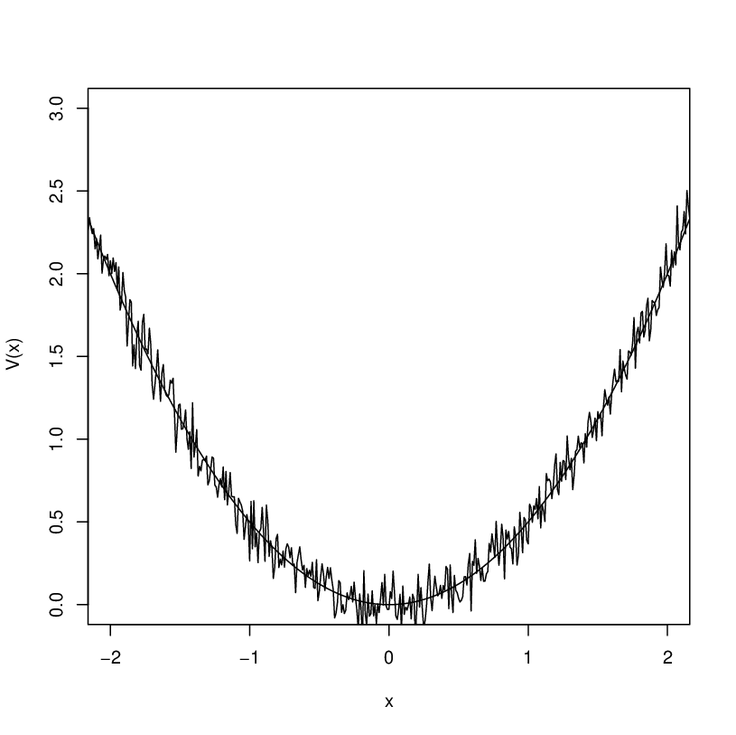
The Wiener process in (26) is defined on another probability space, and we work with the product space and product measure and so is independent of . Note that for the sake of notational simplicity, we have suppressed the dependence of and on for . Under Condition 6.1, for every , there exists a unique strong solution to the SDE (26). In contrast to the periodic case, when equation (26) is used to model the dynamics of a particle in a rough potential, the roughness is due to the “small” randomness generated by the random field . Figure 2 depicts a realization of such a random field superimposed on the smooth potential function . In the figure, is a zero mean Gaussian random field with Gaussian type correlation, i.e., .
Compared with multiscale diffusions with periodic environment, the analysis for general random media is relatively new. To the best of our knowledge, the first attempt to generalize the results obtained for the locally periodic setting to the locally stationary setting probably appeared in the work of [37], which studied random walks on with a locally stationary environment. Extensions have been considered in [42, 43] to diffusions whose generators are self-adjoint and take a certain form.
6.1 Homogenization in One Dimension
As in Section 5, we state the homogenization theorem for the one-dimensional case where everything can be explicitly quantified. For higher dimensions, analogous results exist but explicit calculation is much more difficult. In the following result we assume that is fixed and let tend to zero in order to clearly identify the effect of homogenization. To ease exposition, we temporarily denote by .
Theorem 6.1
Consider the one dimension case and assume Condition 6.1. Then the law of on converges weakly to the law of , in probability with respect to , where is the solution to the SDE
and with
| (27) |
The rest of this subsection is devoted to the proof of this theorem. Since it is very similar to that of [42, Theorem 3.1], we will only give an outline. Without loss of generality, we assume in the proof. We start with the following lemma.
Lemma 6.2
Let be a bounded and measurable function and let be a stationary random field such that
Then as
in , where denotes the expected value with respect to the independent Wiener process but with given, and
Proof. The proof follows from Theorem 6.1 in [42]. The only observation we need to make is that in our case the fast motion is governed by the generator
Then by the discussion in Section 2.2, in particular Theorem 2.1, of [36], the averaging should be taken under the corresponding ergodic stationary probability measure on say which satisfies
for any stationary random field .
Proof of Theorem 6.1. Let be the random field defined by
It is straightforward to verify that and
| (28) | ||||
Define the process
Then Itô’s formula implies that
The latter and (28) imply that is -a.s. a martingale with quadratic variation
It follows now from Lemma 6.2 [taking ] that as
where
Similarly, by Lemma 6.2 [taking ] again we have that
in as . Finally, note that by Birkhoff’s ergodic theorem -almost surely, as . Thus as
-almost surely. Then the desired convergence follows immediately since
in probability with respect to . This completes the proof.
6.2 Importance Sampling Schemes
It is easy to see that the homogenization result in the random case is analogous to that in the periodic case Corollary 5.1 with and replaced by , respectively. By analogy, it suggests that in the one dimensional case satisfies the large deviations principle with rate function given by (24), where
and and are defined by (27). Therefore it is natural to conjecture that given a classical subsolution , the corresponding control takes a similar form
Note that in contrast to the periodic case, the control is random in that it implicitly depends on since the random environment depends on it. Even though the associated importance sampling schemes are shown to be efficient in our empirical study, development of the underlying large deviation theory and a rigorous performance analysis remains to be done.
7 Simulation Results
In this section we test the performance of various Monte Carlo estimators for multiscale diffusions with periodic or random environment. Throughout this section, we assume that the diffusion process is one-dimensional and satisfies the first order Langevin equation (23).
7.1 Simulation Results for Periodic Case
Suppose that we are interested in the Monte Carlo estimation of
for a continuous function and in a periodic environment. We compare three unbiased estimators.
- 1.
The standard Monte Carlo estimator ,
- 2.
- 3.
The importance sampling estimator based on the change of measure corresponding to the control
This is the change of measure based on the control suggested by the homogenized HJB equation without taking into consideration of the multiscale nature of the dynamics. It is independent of the fast variable and differs from the control by a factor .
Based on the theory developed previously, the estimator should outperform the other two estimators as .
For numerical experimentation, we consider the potential function that is drawn in Figure 1, that is, and . Thus the period is . Let
It follows from Corollary 5.1 that the effective drift and diffusivity are
The limiting HJB equation (7) becomes
| (29) |
Under mild conditions that are satisfied here, the unique viscosity solution to this HJB equation equals
where is given by Corollary 5.1 and the infimum is taken over all such that . One can solve this variational problem explicitly and obtain
Since is not smooth at , it is not a classical sense solution. In general one should mollify it in order to produce a smooth subsolution, but it is known (see [46] for an analogous situation) that the bound on performance is still valid if the subsolution is the minimum of two classical sense solutions with a single discontinuous interface. Therefore we can just define the subsolution as the solution and the corresponding controls are
where if and if .
In the numerical simulation, we set , the initial condition , and the terminal time . One can calculate and . We used a predictor-corrector Euler scheme to simulate the trajectories of (23) and the associated controlled SDE. For reasons that will be discussed in Appendix A, a direct numerical approximation scheme was adopted instead of other techniques such as multiscale integrator or projective integrator methods (see [45, 17, 23]). By Theorem 7.1 we know that the error in the Euler approximation is bounded by a term of order , where is the time discretization step. For each choice of and we chose so that the aforementioned error bound is of the order . In other words, we set . Hence, as gets smaller the discretization step becomes smaller as well. Even though by extensive experimentation we found that in general the choice of was crucial for obtaining accurate results, for the periodic example studied here the requirement can be relaxed and a coarser discretization can still lead to accurate and stable results.
Simulations were done using parallel computing in the C programming language. We used Mersenne Twister [35] for the random number generator, with a sample size of . The measure for comparing different schemes is the relative error of the estimators, which is defined as
The smaller the relative error the more efficient the estimator. Since in practice both the standard deviation and the expected value of an estimator are typically unknown, empirical relative error is often used for measurement. In other words, the expected value of the estimator will be replaced by the empirical sample mean, and the standard deviation of the estimator will be replaced by the empirical sample standard error. In order to distinguish among the different Monte Carlo procedures, we denote by the empirical relative error of for . We would like to point out that the expected value in the denominator [which is always due to unbiasedness] is replaced by , regardless of . The reason is that is the most accurate estimate of .
The numerical results are summarized in Table 1. As suspected, the estimator significantly outperforms both the standard Monte Carlo estimator and the estimator which corresponds to the change of measure purely based on the homogenized HJB equation. In particular, the estimator seems to be of bounded relative error, which is a stronger notion of efficiency than asymptotic optimality.
| No. | |||||||||
7.2 Simulation Results for Random Case
In this section we test the performance of the proposed estimator in the case of a random environment by estimating an exit probability. In particular, we again consider the first order Langevin equation (23) in one dimension and wish to estimate the exit probability
where the exit time is defined by
As in the periodic case, we compare the estimator proposed in Section 6.2 [again denoted by with the standard Monte-Carlo estimator and with the estimator that corresponds to the change of measure based just on the homogenized HJB equation.
We consider and to be a zero mean Gaussian random field with covariance function
It follows from Theorem 6.1 that the effective drift and diffusivity are respectively
In this case the limiting HJB equation is the time independent version of (29) defined on the interval
with the boundary condition if and if . We consider the case , initial point and . The maximal viscosity solution (which is also the maximal classical sense subsolution) to this HJB equation is
While this example is not over a finite time interval, the proof of Theorem 4.1 can be adapted as in [15] to yield the analogous results. The importance sampling estimator corresponds to the control
while the estimator corresponds to the constant control
Following the notation of the periodic case, we summarize the simulation results in Table 2. We used the randomization method to simulate the Gaussian random environment. See [28] for an exposition on the simulation of Gaussian random fields.
| No. | |||||||||
As in the periodic case, the estimator outperforms both and . Comparing Tables 1 and 2, the reader may wonder why we did not try combinations of with larger ratio . Extensive empirical studies showed that the direct numerical scheme that we chose to simulate from the SDE was much more sensitive in honoring the rule for choosing the discretization step in the random case than it was for the periodic case. So, due to practical limitation on the computational budget, we had to limit to the values reported in Table 2 in order to obtain meaningful results. Note that this significant computational burden required to produce samples is independent of the scheme, and thus provides further impetus for the development of the theoretically best algorithms.
We also ran simulations for the model
| (30) |
where is the same random field as before and the goal is again to estimate the exit probability
with now , and .
Notice that this corresponds to the (random) potential function that is drawn in Figure 2. The difference between this and the previous model is that here there exists a stable point, in particular at , in the domain of attraction (see Figure 2). The results were qualitatively the same as in Table 2 and are presented in Table 3.
| No. | |||||||||
Appendix A. Numerical Schemes for Multiscale Problems
Assume for simplicity the periodic setup, and denote by the numerical approximation to provided by a direct scheme with weak order of convergence . For such a numerical scheme one has the following error bound, whose proof follows from standard arguments, e.g. [17], and will not be repeated here.
Theorem 7.1
If and the discretization step are such that , then for every and every smooth function with compact support, there exist constants and that are independent of and such that for all satisfying ,
| (31) |
The bound (31) illustrates the computational difficulty in approximating multiscale diffusions. Fix an error tolerance level . The error bound (31) indicates that a time step of order
is needed. The corresponding computational cost per unit of time is , which becomes more expensive as , and become smaller.
Of course, the increasing computational cost highlights the importance of important sampling or other fast simulation techniques for treating these kinds of problems. Since our interest in this work is to study importance sampling and not the numerical methods, we do not elaborate here much on the approximation aspect of the problem. Numerical methods such as multiscale integrator methods [45, 17], and projective integrator methods [23, 38] have been proposed to efficiently simulate systems with widely separated time scales. These methods turn out to be less costly than direct approximation methods, especially when is small. For example, in the case of equation (1) and for , perturbation analysis [17] shows that these methods are less costly than direct approximation when . Observe that in the examples of Section 7, the values of and were not smaller than the overall tolerance error . Hence, we chose to use direct approximation schemes and to rely on parallel computing to carry out the simulation.
Acknowledgments
We would like to thank the Center for Computation and Visualization (CCV) at Brown University for making available to us their high performance computing center.
References
- [1] O. Alvarez and M. Bardi, Viscosity solutions methods for singular perturbations in deterministic and stochastic control, SIAM Journal on Control and Optimization, 40(4), (2001), pp. 1159-1188.
- [2] A. Ansari, Mean first passage time solution of the Smoluchowski equation: Application of relaxation dynamics in myoglobin, Journal of Chemical Physics, 112(5), (2000), pp. 2516-2522.
- [3] P. Baldi, Large deviations for diffusions processes with homogenization and applications, Annals of Probability, 19(2), (1991), pp. 509–524.
- [4] M. Bardi and I. Capuzzo Dolcetta, Optimal Control and Viscosity Solutions of Hamilton Jacobi Bellman Equations, Birkäuser, Boston, 1997.
- [5] A. Bensoussan, J.L. Lions and G. Papanicolaou, Asymptotic Analysis for Periodic Structures, Vol 5, Studies in Mathematics and its Applications, North-Holland Publishing Co., Amsterdam, 1978.
- [6] M. Boué and P. Dupuis, A variational representation for certain functionals of Brownian motion, Annals of Probability, 26(4), (1998), pp. 1641-1659.
- [7] M. Boué, P. Dupuis and R. S. Ellis, Large deviations for small noise diffusions with discontinuous statistics, Probability Theory and Related Fields, 116(1), (2000), pp. 125-149.
- [8] J. D. Bryngelson, J. N. Onuchic, N. D. Socci and P. G. Wolynes, Funnels, pathways and the energy landscape of protein folding: A synthesis, Proteins, 21(3), (1995), pp. 167-195.
- [9] R. Buckdahn and N. Ichihara, Limit theorem for controlled backward SDEs and homogenization of Hamilton-Jacobi-Bellman equations, Applied Mathematics and Optimization, 51 (2005), pp. 1-33.
- [10] M. G. Crandall, H. Ishii and P.-L. Lions, User’s guide to viscosity solutions of second order partial differential equations, Bull. Amer. Math. Soc., (N.S.), 27(1), (1992), pp. 1-67.
- [11] T. Dean and P. Dupuis, Splitting for rare event simulation: a large deviation approach to design and analysis, Stochastic Processes and their Applications, 119 (2009), pp. 562-587.
- [12] P. Dupuis and R.S. Ellis, A Weak Convergence Approach to the Theory of Large Deviations, John Wiley & Sons, New York, 1997.
- [13] P. Dupuis and K. Spiliopoulos, Large deviations for multiscale problems via weak convergence methods, Stochastic Processes and their Applications, (2011), to appear.
- [14] P. Dupuis and H. Wang, Importance sampling, large deviations and differential games, Stochastics and Stochastics Reports, 76, (2004), pp. 481-508.
- [15] P. Dupuis and H. Wang, Subsolutions of an Isaacs equation and efficient schemes for importance sampling, Mathematics of Operations Research, 32(3), (2007), pp. 723-757.
- [16] W.E. and B. Engquist, The heterogeneous multi-scale methods, Comm. Math. Sc., 1(1), (2003), pp. 87-133.
- [17] W. E, D. Liu and E. Vanden-Eijnden, Analysis of multiscale methods for stochastic differential equations. Comm. Pure Appl. Math., 58(11), (2005), 1544-1585.
- [18] S.N. Eithier and T.G. Kurtz, Markov Processes: Characterization and Convergence, John Wiley & Sons, New York, 1986.
- [19] L. Evans, Periodic homogenization of certain fully nonlinear partial differential equations, Proc. Roy. Soc. Edinburgh Section A, 120 (1992), pp. 245-265.
- [20] W.H. Fleming and H.M. Soner, Controlled Markov Processes and Viscosity Solutions, Springer, 2nd Ed., 2006.
- [21] M. Freidlin and R. Sowers, A comparison of homogenization and large deviations, with applications to wavefront propagation, Stochastic Process and their Applications, 82(1), (1999), pp. 23–52.
- [22] C.W. Gear and I.G. Kevrekidis, Projective methods for stiff differential equations: problems with gaps in their eigenvalue spectrum, SIAM Journal of Scientific Computing, 24(4), (2003), pp. 109-110.
- [23] D. Givon, I. G. Kevrekidis and R. Kupferman, Strong convergence of projective integration schemes for singularly perturbed stochastic differential systems, Comm. Math. Sci., 4(4), (2006), pp. 707-729.
- [24] P. Guasoni and S. Robertson, Optimal importance sampling with explicit formulas in continuous time, Finance and Stochastics, 12(1), (2008), pp. 1-19.
- [25] K. Horie and H. Ishii, Simultaneous effects of homogenization and vanishing viscosity in fully nonlinear elliptic equations, Funkcialaj Ekvaciaj, 46(1), (2003), pp. 63-88.
- [26] C. Hyeon and D. Thirumalai, Can energy landscapes roughness of proteins and RNA be measured by using mechanical unfolding experiments?, Proc. Natl. Acad. Sci., USA, 100(18), (2003), pp. 10249-10253.
- [27] I. G. Kevrekidis, C. W. Gear, J. M. Hyman, P. G. Kevrekidis, O. Runborg and C. Theodoropoulos, Equation-free, coarse-grained multiscale computation: Enabling microscopic simulators to perform system-level analysis, Comm. Math. Sci., 1(4), (2003), pp. 715-762.
- [28] P.R. Kramer, O. Kurbanmuradov and K. Sabelfeld, Comparative analysis of multiscale Gaussian random field simulation algorithms, Journal of Computational Physics, 226(1), (2007), pp. 897-924.
- [29] S. Kozlov, The averaging of random operators, Math. USSR Sb, 109 (1979), pp. 188-202.
- [30] S. Kozlov, Geometric aspects of averaging, Russian Math. Surveys, 44 (1989), pp. 91-144
- [31] S.M. Kozlov and A.L. Piatniskii, Degeneration of effective diffusion in the presence of periodic potential, Ann. Inst. H. Poincare Probab. Statist., 32(5), (1996), pp. 571-587.
- [32] S. Lifson and J.L. Jackson, On the self-diffusion of ions in a polyelectrolyte solution, Journal of Chemical Physics, 36, (1962), pp. 2410-2414.
- [33] P.-L. Lions and P.E. Souganidis, Homogenization of degenerate second-order PDE in periodic and almost periodic environments and applications, Ann. Inst. H. Poincaré Anal. Non Linéaire, 22(5), (2005), pp. 667-677.
- [34] D. Mondal, P.K. Ghosh and D.S. Ray, Noise-induced transport in a rough racket potential, Journal of Chemical Physics, 130, (2009), pp. 074703.1-074703.7.
- [35] M. Matsumoto and T. Nishimura, Mersenne twister: a 623-dimensionally equidistributed uniform pseudo-random number generator, ACM Trans. Model. Comput. Simul., 8(1), (1998), pp. 3-30.
- [36] S. Olla, Homogenization of Diffusion Processes in Random Fields, 1994, available at www.ceremade.dauphine.fr/ olla/lho.ps.
- [37] S. Olla and P. Siri, Homogenization of a bond diffusion in a locally ergodic random envirnoment, Stochastic Processes and their Applications, 109 (2004), pp. 317-326.
- [38] A. Papavasiliou and I. G. Kevrekidis, Variance reduction for the equation-free simulation of multiscale stochastic systems, Multiscale Modeling Simulation, 6(1), (2007), pp. 70-89.
- [39] G.A. Pavliotis and A.M. Stuart, Multiscale Methods: Averaging and Homogenization, Springer, 2007.
- [40] G. Papanicolaou and S.R.S. Varadhan, Boundary value problems with rapidly oscillating random coefficients, Colloquia Mathematica Societatis Janos Bolyai 27, Random Fields, Esztergom (Hungary) 1979, North Holland, (1982), pp. 835-873.
- [41] G. Papanicolaou, Diffusion in Random Media, 1994, available at math.stanford.edu/papanico/pubftp/make.pdf
- [42] R. Rhodes, Diffusion in a locally stationary random environment, Probability Theory and Related Fields, 143(3-4), (2009), pp. 545-568.
- [43] R. Rhodes, Homogenization of locally stationary diffusions with possibly degenrate diffusion matrix, Annales de l’Institut Henri Poincaré, 45(4), (2009), pp. 981-1001.
- [44] J.G. Saven, J. Wang and P.G.Wolynes, Kinetics of protein folding: The dynamics of globally connected rough energy landscapes with biases, Journal of Chemical Physics, 101(12), (1994), pp. 11037-11043.
- [45] E. Vanden-Eijnden, Numerical techniques for multi-scale dynamical systems with stochastic effects, Comm. Math. Sci., 1(2), (2003), pp. 385-391.
- [46] E. Vanden-Eijnden and J. Weare, Rare event simulation with vanishing error for small noise diffusions, (2009), submitted.
- [47] R. Zwanzig, Diffusion in a rough potential, Proc. Natl. Acad. Sci. USA, 85, (1988), pp. 2029-2030.