Heat transport in silicon from first principles calculations
Abstract
Using harmonic and anharmonic force constants extracted from density-functional calculations within a supercell, we have developed a relatively simple but general method to compute thermodynamic and thermal properties of any crystal. First, from the harmonic, cubic, and quartic force constants we construct a force field for molecular dynamics (MD). It is exact in the limit of small atomic displacements and thus does not suffer from inaccuracies inherent in semi-empirical potentials such as Stillinger-Weber’s. By using the Green-Kubo (GK) formula and molecular dynamics simulations, we extract the bulk thermal conductivity. This method is accurate at high temperatures where three-phonon processes need to be included to higher orders, but may suffer from size scaling issues. Next, we use perturbation theory (Fermi Golden rule) to extract the phonon lifetimes and compute the thermal conductivity from the relaxation time approximation. This method is valid at most temperatures, but will overestimate at very high temperatures, where higher order processes neglected in our calculations, also contribute. As a test, these methods are applied to bulk crystalline silicon, and the results are compared and differences discussed in more detail. The presented methodology paves the way for a systematic approach to model heat transport in solids using multiscale modeling, in which the relaxation time due to anharmonic 3-phonon processes is calculated quantitatively, in addition to the usual harmonic properties such as phonon frequencies and group velocities. It also allows the construction of accurate bulk interatomic potentials database.
pacs
63.20.-e,63.20.dk,63.20.kg,61.50.AhI Introduction
Classical molecular dynamics (MD) simulations use either semi-empirical potentials such as Stillinger-Weber (SW)[1], Abell-Tersoff-Brenner[2] or other type of force fields where the potential energy is an analytical function of the atomic positions, or first-principles potentials calculated typically using density-functional methods based on either the Born-Oppenheimer[3] or the Car-Parrinello[4] dynamics. The former are fast to compute but suffer from inaccuracies, while the latter are accurate but time-consuming to compute. Due to recent interest in thermal transport in semiconductor materials having good thermoelectric properties and the topic of microelectronics thermal management in general, there have been many calculations of the lattice thermal conductivity of materials using the Green-Kubo (GK) formula[5, 6]. This formula relates the thermal conductivity, through the use of the fluctuation-dissipation theorem, to the time-integral of the heat current autocorrelation function. The latter is calculated from an MD simulation, and the ensemble average is usually replaced by a time average. Semi empirical potentials such as SW are usually used to perform the MD simulation for a system such as Si. As the thermal conductivity of a perfect crystal is mainly due to anharmonic three-phonon processes, directly related to the third-derivatives of the potential energy with respect to atomic displacements, and the latter is generally not fitted or considered in the design of the semi-empirical potentials, there is really no good reason to expect an accurate value for the thermal conductivity calculated from a GK-MD simulation. In the case of Si, when using the SW potential, however, for some reason[7], relatively good agreement is found between the experiment and the simulation results, even for a relatively small supercell[8, 9, 10, 11]. The latter fact is also cause for concern, because, as we will show in the following, a small supercell limits the number of long-wavelength phonons which carry a large portion of the heat in a material. The lucky agreement can be attributed to a cancellation due to two different effects, which will be discussed in sectionIII.2. Sellan et al.[11] have presented a discussion on convergence issues, mostly with respect to non-equilibrium MD simulations, and we will also discuss the scaling issue with respect to GK-MD and lattice dynamics (LD) in this paper.
More accurate calculations of the thermal conductivity, based on the full solution of Boltzmann transport equation have shown that the thermal conductivity of Si using the SW potential is about 4-times larger than the experiment, while using the Tersoff or EIDP potentials produce results that are about twice larger than the experimental values[12]. In a similar work, using the environment-dependent interaction potential (EDIP), Pascual-Gutierrez et al.[13] also find thermal conductivity of bulk Si from MD in good agreement with experiments. In a subsequent work[14], the same group computed the thermal conductivity using the lattice dynamics (LD) theory based on the same EDIP potential, similar to the work of Broido et al. [12]. They obtain good agreement with experiments whereas Broido et al. do not. The reason for this discrepancy, as they also mention in their paper, is unclear. Opinions on the accuracy of semiempirical potentials seem to differ as there have been other reports[15] where SW is found to overestimate the thermal conductivity by 70%. As we will show in this paper, some of these potentials might not be completely reliable for the calculation of the thermal transport properties for the simple reason that they were not fitted or constructed to have the correct third derivatives, which are responsible for the thermal resistivity of a material. In fact even their harmonic force constants produce phonon dispersions and elastic constants which differ from experiments by 10 up to 40%. Furthermore such potentials exist and have been thouroughly tested for only a very small number of pure crystalline solids.
In a tour de force work, Broido et al., later, used the density-functional perturbation theory (DFPT) formalism in order to calculate the phonon scattering rates from first-principles DFT calculations and were able to successfully reproduce the thermal conductivity of bulk Si and Ge[16]. Their approach, which was very accurate, included the calculation of all the cubic force constants up to 4 lattice parameters away, and the complete iterative solution of the Boltzmann transport equation.
We recently developed a methodology to extract second, third and fourth derivatives of the potential energy from first-principles calculations[17], and showed that the phonon dispersion relation in Si can be well-reproduced. In this paper, we pursue this work further and use these derivatives to construct a force field in order to explore the results from MD simulations and perturbation calculation to calculate the thermal conductivity of bulk Si. We should mention that our approach, even though very similar in essence to that of Broido et al., is simpler in the sense that it limits the range of the force constants (FCs) to a few neighbors (5 for harmonic and 1 for cubic in the present case study of Si, in contrast to more than 20 for harmonic and 10 for cubic in the work of Broido et al.[16]). For the sake of physical correctness, however, we enforce the translational, rotational and Huang invariances on the extracted force constants. So the latter are not exactly equal to the ones obtained from DFPT or any finite difference calculation of the forces, but make the calculation load much lighter than if one had to include so many neighbors. On the other hand a DFPT calculation, if restricted to few neighbors, should enforce all these invariances. Usually, only the translational ones, also known as the “Acoustic Sum Rule” (ASR) are enforced in some of the standard DFT codes such as Quantum Espresso[18].
In what follows we briefly review the methodology to extract force constants from first-principles density-functional theory calculations (FP-DFT). The formalism for the molecular dynamics and Green-Kubo calculations of are explained in section (III). This will be followed by the lattice dynamics approach detailed in section (IV). Results for Si will be shown and discussed in section (V), followed by conclusions.
II Extraction of force constants from FP-DFT calculations
We construct the potential energy for the MD simulation as a Taylor expansion up to fourth order in the atomic displacement of atom about its equilibrium position:
| (1) | |||||
| (2) |
The last equation defines the on-site energy . If the displacements are around the equilibrium position, and this is usually the case, . The coefficients and in the expansion are called the harmonic, cubic, and quartic force constants respectively, and satisfy certain symmetry constraints. Namely they must be invariant under interchange of the indices, uniform translations and rotations of the atoms, in addition to invariance under symmetry operations of the crystal. The details of the needed constraints and how they are imposed can be found in our previous work[17].
To get these numbers, we consider one or several supercells in which atoms are in their equilibrium position. One, two or three neighboring atoms are moved simultaneously by a small amount, typically about along the cartesian directions. Consideration of crystal symmetry usually reduces the needed displacements. For instance in a cubic-based crystal, like silicon, where the two atoms in the primitive cell are equivalent, one only needs to move one Si atom along the x direction. This is sufficient to extract all harmonic force constants if the supercell size is large enough. The latter size is chosen depending on the available computational power and the considered range of force constants. To get three- and four-body interaction terms, one needs to move two and three atoms at a time and record the forces on all atoms in the supercell. It is advantageous to record forces for atomic displacements in two opposite directions as there would be cancellation of the cubic contributions and this would make the calculation of the harmonic FCs much more accurate (up to order ). Thus one would obtain a large set of force-displacement relations computed from a FP-DFT code. Together with the invariance constraints, an overcomplete linear set of equations on all the force constants will be formed. A singular-value decomposition algorithm is then used to solve this linear overcomplete set. We find that usually the violation of the invariance relations is of the order of times the FC itself. This however requires very accurate evaluation of the forces, meaning that they should have converged with respect to the cutoff energy and number of k-points to within at least 4 significant figures, if not more! Our experience on graphene[19] and silicon (present work and reference [[17]] has shown that the harmonic force constants are usually reproduced quite accurately. Higher order FCs have less accuracy as their contribution shows up in the second or third or fourth significant figures of the forces. The main approximation is in cutting off the range of the interactions, which will lead to inaccuracies in some of the Gruneisen parameters as we will shortly see.
III Molecular dynamics and the Green-Kubo formalism
Typically a supercell is constructed with periodic boundary conditions, and an MD simulation is performed over a long enough time steps in order to reach thermal equilibrium, followed by a long (N,V,E) simulation in order to collect data on for later statistical processing, i.e time and ensemble averaging of its autocorrelation.
Based on the potential displayed in Eq. (2), one can extract the expression for the force, required in the MD simulations:
The heat current is defined in the discrete (atomic) case of a lattice, where there is no convection, as:
| (3) |
where is the velocity of particle and , as defined in Eq. (2) is the local energy of atom . Using our expansion, it can be expressed as a function of the force constants as follows (as we expand around the equilibrium position, we assume ) :
| (4) | |||||
This definition leads to the following form of the local heat current:
| (5) | |||||
| (6) |
where , and denotes the equilibrium average of the observable , which in the classical case can be replaced by its time average provided the time is long enough to satisfy ergodicity. The ensemble averaging is necessary as long as different runs starting with different initial conditions lead to different integrated autocorrelation functions. The true current autocorrelations decay quite fast. In a single MD run, however, this decay is not observed. Instead one observes a decay in the amplitude followed by random oscillations about zero. As finite systems are usually not ergodic, an ensemble average, over the random initial conditions is also needed to correctly simulate the equilibrium average required in the Green-Kubo formula. In this case, the ensemble-averaged autocorrelation function will decay smoothly to zero with time. One will then see that the decay is indeed relatively short, because the long-time tails get cancelled after ensemble averaging. The advantage of the ensemble averaging, in addition of course to the usual time averaging, is that one samples the phase space more randomly, and generates uncorrelated sets of pairs for a given time difference . In this case, the mean has the convergence properties of gaussian-distributed variables and the error decays to zero as the inverse square root of the number of initial conditions.
In a numerical simulation, the GK formula should be replaced by:
| (7) | |||||
where is the total simulation time of each run, is the time difference between two successive data points, and are integers labeling time, and is the number of generated initial conditions, each labeled by . One important comment is in order here, and that is the use of in the denominator instead of the more intuitive which is the actual number of terms in the last sum. One can show that the choice in Eq. (7) provides an unbiased estimator of the autocorrelation[20]. Some previous works in the GK method such as reference [9] have used the “biased” formula, which would be fine as long as the total simulation time is much larger than the largest time used for the integration. One simple way to become convinced that Eq. (7) is the correct way, is to consider large times near the maximum simulation time . As and are both fluctuating random numbers, and there are not enough terms in the sum to make the average go to zero, the time average will become large again and tend to instead of decaying to zero as approaches . A division by the small number would not solve the problem, whereas the division by would make this very small as it should.
The simulation time being usually quite long, the statistical error in the time averging is usually small, and we estimate the error bars in our data from the ensemble averaging: If is the ensemble-averaged autocorrelation function, its error bar is evaluated as:
The magnitude of this error bar and the required accuracy in the results determine how many ensembles are needed for a proper estimation of thermal conductivity.
III.1 How many MD steps are necessary?
For a given supercell size, there is a discrete number of phonon modes which can propagate and get scattered in the system. The largest wavelength consistent with the periodic boundary conditions would be the supercell length. To this, one can correspond a smallest phonon wavenumber or frequency allowed in the simulation: . The total simulation time should be large enough so that all phonon modes can get scattered a few times within the simulation period. Largest relaxation times belong to acoustic modes, and usually decay as the inverse square of the phonon frequency. Knowing the smallest allowed frequency due to the finite size of the system, one can estimate the corresponding phonon lifetime (using Klemens’ formula displayed in Eq. (8) for instance). The total MD simulation time should therefore be a few times larger than the largest phonon lifetime so that scattering events of long wavelength phonon modes can properly be sampled during the MD run. As an example, we can consider Si system in a cubic 10x10x10 supercell of 8000 atoms. In this case nm corresponding to which is a fifth of the line. The lowest frequency mode is therefore about THz. As can be seen in Fig. (5) below, the normal and umklapp lifetimes at this frequency are 3000 ps and 10000 ps respectively, leading to a total lifetime of 2300 ps. So in order to sample such rare events, one needs to calculate the autocorrelation over at least 20 ns, which means the MD simulation should be run for at least the same amount of time if not longer. This could be computationally prohibitive. If the runs are made with fewer MD steps long wavelength phonons will not be relaxed and the autocorrelation would not tend to zero. Another consequence of this remark is that for large supercells, as relaxation times scale as , longer simulation times proportional to the square of the the supercell size would be required.
III.2 Size scaling
As mentioned, the choice of a finite supercell comes with the cost of discretizing the phonon modes and supressing the phonons of wavelengths longer than the supercell length. The neglected contribution maybe estimated as follows: the anharmonic lifetime of acoustic modes maybe approximated by the Klemens’ formula [30]
| (8) |
where is the largest frequency of the branch , the mode Gruneisen parameter, the frequency, and the group velocity associated with the mode . Therefore long wavelength phonons will have a large relaxation time and can considerably contribute to the thermal conductivity. Assuming this form in the relaxation time approximation to the thermal conductivity, and using Eq. (16), we can write the thermal conductivity as a sum over contributions of phonons of different frequencies:
In 3D, since the density of states (DOS) is quadratic in frequency, the contribution of long wavelength acoustic phonons would be linear in the cutoff frequency :
For low frequencies and so that
| (9) | |||||
where and are constants which do not depend on the size, is the mean free path (MFP) associated with the cutoff frequency . This gives us a way to deduce how the thermal conductivity of a finite size sample scales with the supercell length or the cutoff frequency or MFP, . We should note that a different scaling law () was also proposed and used by Sellan et al.[11], and also Turney et al.[21] when they want to extrapolate their thermal conductivity data to infinite size. The argument they used to deduce it however was based on the Matthiesen’s rule, stating that the bulk resistivity is obtained by adding the finite size resistivity to the one obtained from taken as relaxation time.
There is another additional problem with finite size MD simulations. Even though momentum is still conserved in a 3-phonon process, because the modes are discrete in a finite supercell, energy conservation will not always be possible, unless the energy difference where is on the order of the sum of inverse lifetimes of the three considered phonons. If this relation is not satisfied, the considered 3-phonon scattering will not take place in a finite supercell, and this will lead to an overestimation of the lifetime of the phonons, and thus, of the thermal conductivity.
These competing effects, namely an overestimation of due to limited phase space for energy conservation and an underestimation due to cutoff of low frequency acoustic modes, may lead to a magical cancellation, resulting in thermal conductivities in good agreement with experiments even for moderate supercell size. This error cancellation will likely affect the temperature-dependence of : at higher temperatures the discreteness error is reduced as increases linearly with . The frequency cutoff error, however, will not be affected by high temperatures. Consequently, as is increased the thermal conductivity of a finite sample will decrease faster than with temperature. This has been observed in the work of Volz and Chen[8]. It can also be verified by introducing other scattering events such as isotope or defect scattering leading to larger values. In such cases, the discreteness of modes will have little effect, and the simulated will be less than the exact one, due to the cutoff of long MFP phonons effect. As a result, in a system where due to disorder or high temperatures scattering rates are high, GK-MD simulations will typically require larger supercells to converge.
The correct way of estimating is to do a proper size scaling at each temperature by plotting versus and linearly extrapolating to .
IV The Lattice Dynamics approach
Using the extracted for constants, one can form the dynamical matrix of the crystal using its primitive cell data:
| (10) |
where is a translation vector of the crystal, refers to an atom in the primitive cell, and are cartesian components . Such sums of the force constants over the translation vectors of the primitive lattice are usually short-ranged and fast to compute, except if Coulomb interactions are involved, in which case the sum is evaluated using the Ewald method.
Diagonalizing this matrix, one can find the phonon spectrum and the normal modes as its eigenvectors:
| (11) |
where labels a phonon band (or branch), and refers to a point in the first Brillouin zone (FBZ). Using these eigenvectors and eigenvalues, and from perturbation theory, one can calculate the phonon lineshifts and lifetimes as the real and imaginary parts of the 3-phonon self-energy defined as[24, 25, 26, 27]:
| (12) |
where , is a small infinitesimal number, which in practice is taken to be finite for a given k-mesh size, n is the equilibrium Bose-Einstein distribution function, and 1 and 2 refer to modes and . The 3-phonon matrix element , expressed as a function of the cubic force constants , is given by:
| (13) |
The calculation of the self-energy would require a double sum over the q-points (labeled above by 1 and 2) in the FBZ . Due to the conservation of momentum, however, only terms with , with being a reciprocal lattice vector, should be included in the above sum. In practice, therefore, this involves only a single summation. To get the phonon dispersion and lifetimes due to 3-phonon scattering terms, one needs to solve where is the real part of the self-energy () . This equation needs to be solved iteratively. Since the shift is usually small, to leading order, one can use i.e. one uses the on-shell frequency as argument of the self-energy. The same approximation will be used for the imaginary part giving the inverse lifetimes. The corresponding phonon lifetime will be given by . In the evaluation of the imaginary part , one encounters Dirac delta functions reflecting the conservation of energy in the three-phonon process: . In effect, from Eq. (12), it can be noticed that the delta function is substituted by a Lorentzian function of width . The latter depends on the choice of the k-point mesh in the FBZ. A small value for can be used for a fine mesh, while a coarse mesh requires larger values of . Typically is chosen to be of the order of energy spacing in the joint density of states (JDOS) so that the latter is a smooth function of the frequency and does not display any oscillations with sharp peaks which would appear if the width is too small.
| (14) |
The anharmonicity can be characterized by the Gruneisen parameters (GP). The force constant GP is defined as -d ln d ln where is the volume. The mode GP is defined as: = -d ln d ln where is the phonon frequency evaluated at the point and band index . It gives the relative decrease in the phonon frequency as the volume is increased by 1%. From the Taylor expansion of the harmonic force constants in terms of the volume or the lattice parameter, one can calculate such change.
| (15) | |||||
where is the equilibrium atomic position of atom type in the primitive cell labeled by the translation vector .
Finally, the thermal conductivity is calculated within the relaxation time approximation (RTA), which leads to the following well-known expression for the thermal conductivity:
| (16) |
where is the volume of the unit cell. The relaxation time in this expression represents the time after which a phonon in mode reaches equilibrium on the average, and depends on the scattering processes involved. In a pure bulk sample, the only source of phonon scattering is anharmonicity dominated usually by three-phonon processes. Using perturbation theory or the well-known Fermi Golden rule (FGR), one can derive the expression of the relaxation time as a function of the cubic force constants[24, 25, 26, 27]. It can be shown that to a good approximation, it is given by
| (17) |
In what follows, we have disregarded the boundary scattering term, which is responsible for the low-temperature behavior of . In such case, is expected to saturate to a finite value at low enough temperatures. The reason for this saturation can be understood if one assumes the low-frequency limit of the DOS and the relaxation times similar to Eq. 9. Considering that in limit we have: and (with ), and the relaxation time can be written as , the integral defining the thermal conductivity can be transformed, in the low temperature limit, to:
The constant that appears in the low energy limit of the relaxation time as well as the speeds of sound determine the saturated value of the thermal conductivity. So when only 3-phonon scattering processes are included, the thermal conductivity would tend to as goes to 0.
Finally, in our numerical calculations where the integral in the FBZ has been approximated by a sum over a discrete set of k-points, the low-frequency region is not properly sampled and we observe a decay to zero at low , and therefore have not reported the unreliable low-temperature data in this work.
V Results and Discussions
V.1 Validation of force constants
First-principles calculations were done using the PWSCF code of the Quantum Espresso package[18] A set of force-displacement data were calculated using supercell of 64 Si atoms. The set of force-displacements data, along with the symmetry constraints, form an over-complete linear set of equations needed to determine the potential derivatives. We use the local density approximation (LDA) of Perdew and Zunger[22] with a cutoff energy of 40 Ryd and 10 k-points in the irreducible Brillouin zone of the cubic supercell. The range of different ranks of force constants can be chosen by the user. We have set the range of harmonic forces constants (FCs) to 5 nearest neighbor shells, and that of the cubic and quartic force constants to the first neighbor shell only. This results in 17, 5 and 14 independent harmonic, cubic and quartic FCs respectively. The corresponding number of terms in the Taylor expansion of the potential energy are, however, equal to 1500, 1146 and 7980 respectively. This is why the ranges were restricted to 5, 1 and 1 nearest neighbor shells in order to limit the computational time to a reasonable amount. Note that despite the large number of terms to be computed, arithmetic operations are only limited to additions and multiplications.
In Fig. (1), we show the change in the total energy as an atom in the supercell is moved along the [100], [110] and [111] directions respectively. Resutls from DFT calculations are compared against our developed force field including the harmonic, harmonic+cubic, and harmonic+cubic+quartic terms of the Taylor expansion. For the sake of comparison, we have also plotted the same energy change ontained from the Stillinger-Weber (SW) potential[1], which is widely used in MD simulations of Si systems.


To further assess the accuracy of the force field, we have also moved all the atoms in the supercell in different random directions by a small amount of magnitudes 0.1 and 0.2 respectively, and compared the average force of our model and the SW potential to the FP-DFT one. The deviation is charaterized by:
| (18) |
The results for the parameter are summarized in table (1).
| Amplitude() | (SW) | (Present) |
|---|---|---|
| 0.1 | 0.35 | 0.05 |
| 0.2 | 0.28 | 0.08 |
We can notice that this type of error estimate would also include contributions from many-body forces, and is a more stringent test on the force field. The errors from the present model are consistently about 4 to 5 times smaller that the SW potential.
In the following we follow two paths to compute the thermal conductivity. The first is to use the Green-Kubo formula, by using the results from an MD simulation:
V.2 Thermal conductivity from MD-GK
As previously mentioned, there will be large fluctuations in the current autocorrelation function versus time from one run to the next, and therefore an averaging over several initial conditions is necessary to produce a reliable plot. In Fig. (2), we have plotted such ensemble average for a 10x10x10 supercell containing 8000 atoms. The error bars are mainly due to the ensemble averaging, and those related to the time averaging are small as the number of MD time steps are quite large.
We can also see in this figure the cumulative integral of the ensemble-averaged autocorrelation function. The same calculation was performed in a 7x7x7 supercell of 2744 atoms, where the averaging was over 99 runs with different initial conditions. Due to its larger size, there are smaller fluctuations in the average current per atom in the 10x10x10 supercell, and we only used 27 initial conditions for this supercell. Since from each MD run one can really extract three autocorrelation functions , and , which are equal by cubic symmetry, we also averaged over the 3 directions. In this sense, the above mentioned numbers should be multiplied by 3.

The error bars are determined by the large fluctuations in the integrated autocorrelations divided by the square root of the number of ensembles. The error bar due to the time average is usually much smaller if MD simulations are run for a long enough time.
The results for two different supercell sizes are summarized in table (2) as compared with the experimental data of Slack et al.[28]. One can notice an underestimation of the experimental data, which is reduced as the supercell size is increased. To get the correct value in the thermodynamic limit, one needs to extrapolate these results to infinite size.
| Supercell size | MD-GK | LD | experiment |
|---|---|---|---|
| 7x7x7 | 37 10 | 32.67 | 64 3 |
| 10x10x10 | 43 12 | 47.2 | 64 3 |
There are a few competing effects which can explain this discrepancy: the most important one is size effect, which as was just explained, underestimates . Similarly, the larger value of the Gruneisen parameter for the acoustic modes in our model will produce a smaller relaxation time (see the Klemens formula in Eq.(8)).
The following effects will, however, lead to an overestimation of the thermal conductivity: in the classical MD simulations, the number of modes is the high-temperature limit of the Bose-Einstein distribution, which is larger than the quantum distribution. This leads to a heat capacity per mode of and therefore an overestimate of the true heat capacity (see also Fig. (8)). In a finite size cell, the allowed frequencies are quantized and energy conservation after a 3-phonon process can never be exactly satisfied, this will lead to an effectively longer lifetime for phonons, and thus also overestimate . It is not easy to quantify these errors except for those due to the phonon occupation numbers. It is therefore possible that there is a cancellation. In our case, since only two supercell sizes were considered, we can not do a systematic size scaling study, but overall, due to these cancellations the MD-GK results seem to be weakly dependent on size, in agreement with previous MD simulations (see for example Table I in reference [[11]]).
Here, we must point out some discrepancy between published results on Si using the SW potential. Using the MD-GK method, Philpot et al. and Volz et al. [9, 8] find a thermal conductivity in reasonable agreement (to within 30%) with experiments. Broido et al.[12], on the other hand, have shown by solving Boltzmann equation beyond the RTA, that . Recently Sellan et al.[11] investigated size effects in GK-MD simulations, direct method, and also used lattice dynamics to compute the thermal conductivity of Si from the SW potential. They found that , which is only 70% larger than the experimental value of 80 W/mK, in contrast to Broido et al’s [12] prediction. Their direct method followed by scaling predicts W/mK, and their unscaled GK value for a 8x8x8 supercell is ( W/mK).
All these results point to the subtleties involved in extracting a reliable value for the thermal conductivity of bulk materials, no matter what method is used.
To investigate this discrepancy, we used our approach to extract cubic force constants from the SW potential and used LD theory to compute the corresponding thermal conductivity. Using the same k-point mesh, in order to avoid systematic errors, in comparison to FP-derived force constants, we found that at 150K the thermal conductivity derived from SW is 80% larger than the one derived from FP-DFT calculations.
V.3 Phonons, DOS and Gruneisen parameters
In extracting the force constants, we have limited the range of the harmonic FCs to 5 neighbor shells, and that of the cubic and quartic terms to one neighbor shell, so that MD simulations can be done within a reasonable time. Using the harmonic FCs, we can obtain the phonon spectrum. As can be seen in Fig. (3) the speeds of sound and most of the features are reproduced with very good accuracy. It is well-known that in order to reproduce the flat feature in the TA modes near the X point, one must go well beyond the fifth neighbor. For the band structure and the density of states (DOS), the overall agreement is good, except for the Gruneisen parameters of the TA branch, where our calculations, which only include cubic force constants up to the first neighbor shell, overestimate TA). Based on Klemens’ formula (Eq. (8)), one might anticipate that our model will slightly underestimate the lifetime of TA modes and thus their contribution in the thermal conductivity.

V.4 Phonon lifetimes and mean-free paths
To get an idea about the relative contributions of the matrix elements, representing the strength of the 3-phonon interactions, versus the phase space available for these transitions, characterized by the two-phonon DOS, we show in Fig. (4) the plots of these quantities. We define the contribution of the matrix elements as:
| (19) |
From Fig. (4) we can note that optical phonons have a much larger weight coming from the matrix element . This explains why they have such a larger relaxation rate compared to acoustic modes for which the matrix elements contribution is very small. The two-phonon DOS is representative of the phase space available for the transitions, and is defined as:
| (20) |
From Fig. (4) it can be inferred that one phonon absorption or emission () dominates for low frequency phonons (acoustic), while two-phonon absorption or emission () dominates at high frequencies (LA and optical).

Next, we show in Fig. (5) the calculated lifetimes of the 3 acoustic and optical modes versus frequency for a regular mesh of kpoints in the first Brillouin zone, at T=70 and 277K. The results depend slightly on the number of k-mesh points used for the integration within the FBZ. Here, we are showing results obtained with 18x18x18 mesh, which is close to convergence. The normal and umklapp components of the lifetimes are separated as . We can note that although the lifetimes associated with normal processes are in , those of umklapp processes seem to scale at low frequencies like so that the former dominates at low frequencies. This is in contrast to the first-principles results provided by Ward and Broido[31] where they report that the umklapp rate is in . Even though not explicitly mentioned in their paper[32], fits to their data with was almost as good as the fit with . In the appendix, we provide a proof why in the case of Si the umklapp rate would behave as .

From Fig. (5), we can notice that at low frequencies (typically below 3 THz or 100 cm-1 where dispersions are linear), normal rates dominate while at higher frequencies and typically for optical modes, umklapp processes dominate transport.
V.5 Thermal conductivity from lattice dynamics
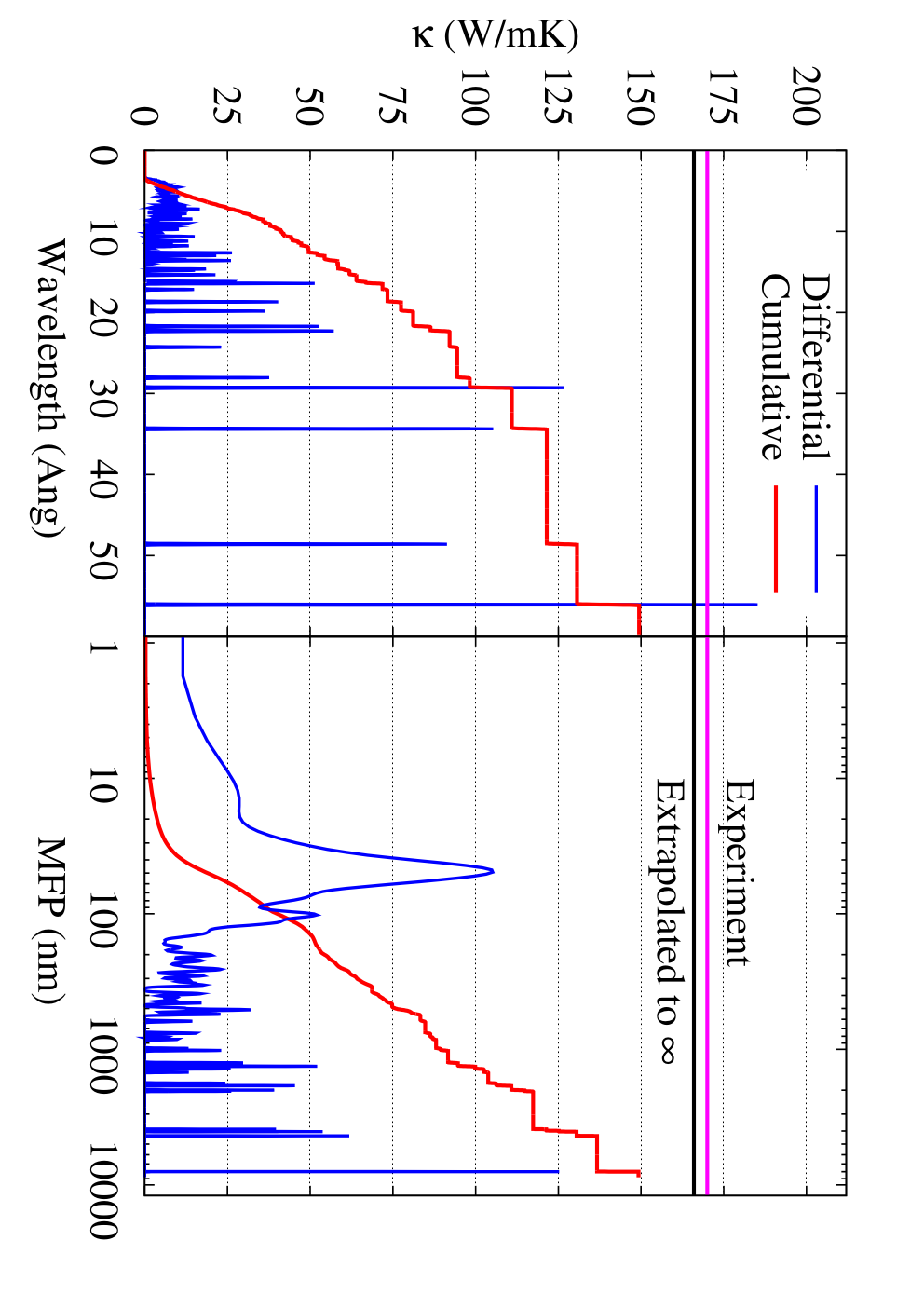
To see what is the contribution of each MFP to the total thermal conductivity, following the approach of Dames and Chen[33], we have decomposed the thermal conductivity based on each mode and sorted each component according to their mean free paths. One can then define a differential thermal conductivity and the accumulated one, which is its integral:
| (21) |
The above can be plotted versus the MFP, , seen as an independent variable. Fig. (6) shows such contribution at 277 K. Considering the extrapolated value to be 166 W/mK, one can notice that MFPs extend well beyond 10 microns even at room temperature. MFPs longer than 1 micron contribute almost to half of the total thermal conductivity! One should also note that the range of MFPs in Si at least, span over 5 orders of magnitude from a nanometer to 100 microns at room temperature. This would be larger as we go to lower temperatures.
To get an acurate estimate of the thermal conductivity, one needs to extrapolate the data obtained from a finite number of k-mesh points, according to Eq. (9). The extrapolated thermal conductivity versus temperature is plotted in Fig. (7) and compared to the experimental results of Glassbrenner and Slack [28] and Inyushkin et al.[29]. We can notice that at low temperatures, boundary scattering limits the experimental thermal conductivity. The agreement is very good in the temperature range of 100 to 500K, after which experimental results decay faster due to higher order phonon scatterings which are like or higher. Our resutls are within the relaxation time approximation, but one could also go beyond and iteratively solve Boltzmann equation as Broido et al. have done[16]. They have shown that for Si and Ge, there would be about a further increase in .

To assess the effect of the classical approximation, which is made in classical MD simulations, we have also compared in Fig. (8) for a given k-point density, the classical and the quantum thermal conductivities within the RTA. They are displayed with symbols on the lines. The quantum one is given by Eq.(16), and the classical one uses the same expression in which the Bose-Einstein distribution is substituted by both in the heat capacity and in the relaxation time. We can notice that the difference is small above the Debye temperature, as expected, but the classical value overestimates the quantum one by 10 to as the temperature is lowered further. This is a combination of the larger heat capacity and a smaller lifetime in the classical case. We have also plotted the contribution of each mode to the thermal conductivity. We can note that at low temperatures maily the two TA modes equally contribute to , whereas at temperatures above 200 K, LA and TA modes equally contribute about almost 1/3 of the thermal conductivity, while LO’s contribution is about 5%.

The computation of the thermal conductivity using the RTA is to some extent more straightforward than the use of GK-MD. The former involves a double summation in the FBZ and has very little systematic error in it, whereas the MD simulations require an ensemble averaging process with a relatively large error bar, not to mention the much longer CPU time needed to run the MD simulations.
VI Conclusions
Using first-principles calculations, we developed a classical force field which was used both in a molecular dynamics simulation and in the calculation of anharmonic phonon lifetimes. Both methods provided an estimate for the thermal conductivity of pure crystalline silicon. The results of these two methods agreed for the same system size in the case where was evaluated in the classical limit. GK-MD is however much more time-consuming and includes large statistical errors. Furthermore it does not provide much information besides the way the integrated autocorrelation converges with simulation time. Size effects were discussed and arguments were provided why equilibrium MD simulations converged relatively fast with respect to the supercell size. Lattice dynamics, on the other hand, proved to be faster, more accurate, and contain more useful information. The use of a linear extrapolation versus the inverse of the size led to a surprizingly good agreement with experiments. Such extrapolation is justified for relaxation rates which are quadratic in frequency at low frequencies. The decomposition of into the contribution of different mean free paths showed that in Si MFPs span over 5 orders of magnitude from 1 nm to 100 microns at room temperature, where about half of the thermal conductivity comes from MFPs larger than 1 micron.
The developed potential has the advantage of being amenable to systematic improvement by including more neighbor shells at the cost of heavier calculations. The approach of using the FGR for the estimation of relaxation rates and the RTA or an improved approximation to by solving the linearized Boltzmann equation, allows one to obtain a relatively accurate estimate of the thermal conductivity of an arbitrary bulk crystalline structure from a few force-displacement relations obtained using first-principles calculations, without any fitting parameters. This method paves the way for an accurate prediction of thermal properties of nanostructured or composite materials in a multiscale approach, which takes as input the relaxation times due to anharmonicity and defect scatterings.
VII Acknowledgements
The authors wish to acknowledge useful discussions with Junichiro Shiomi, Joseph Feldman, Peter Young, and Asegun Henry. We thank Nuo Yang for providing the SW force-displacement data used in Fig. (1).
This work was supported as part of the Solid-State Solar-Thermal Energy Conversion Center (S3TEC), an Energy Frontier Research Center funded by the U.S. Department of Energy, Office of Science, Office of Basic Energy Sciences under Award Number DE-SC0001299.
VIII Appendix
In this appendix, we show the frequency-dependence of the umklapp rates. According to Eq. 12, the relaxation rate is a product of the 3-phonon matrix element , a combination of occupation factors, and delta functions reflecting the constraints of energy conservation. We will separately discuss the frequency dependence of the matrix element and the phase space term.
First, the sum over the second momentum 2 is cancelled by the constraint of momentum conservation, so that the relaxation rate is just the 3D integral over in the FBZ. One of the dimensions can be integrated over by using the identity
| (22) |
where is the solution of . Note that the denominator containing the group velocities is not small as as long as refer to two different branches; but in case , the denominator becomes linear in .
Second, for umklapp processes, in the small limit, we must have both and near the Brillouin zone boundary such that is inside the zone and outside; so that the corresponding frequencies are not infinitesimally small, but their difference would be. In general, this forces the surface integral to be limited to a pocket of dimensions located at the FBZ boundary, so that the surface integral is of the order of . But in case where there is a degenerate band at the zone boundary, the surface would be of order instead. Different cases based on the symmetry of the crystal and the type of degeneracy have been discussed in detail by Herring[34]. In our case of interest, namely Si, it is possible to have a 3-phonon process involving a small momentum acoustic mode connecting the LA branch to the LO one, with which it is degenerate, near the Brillouin zone boundary all along , with a surface area , therefore, of order .
Third, among the two types of terms: phonon decaying to and one phonon absorption , the former cannot contribute because and and are finite. Therefore only the terms contribute to the umklapp lifetimes at small frequencies. In the latter, one can substitute by . We must remember to substitute the argument in the relaxation rate by its on-shell value . So that, in the limit of low frequencies, the inverse lifetime can be written as:
| (23) |
Finally, due to the odd parity of the cubic force constants, one can show that for small we have .
Putting everything together, we find that the umklapp rates at low frequencies are, to leading order, of the form:
| (24) |
This is in agreement with our numerical findings.
For normal processes, there is no restriction for modes 1 and 2 to be near the BZ boundary. For instance, in the (LA LA + TA) process the term contributes and will not be linear in . In such cases the rate would be in and would dominate terms with higher powers of .
References
- [1] F. H. Stillinger and T. A. Weber, Phys. Rev. B 31, 5262 (1985).
- [2] G. C. Abell, Phys. Rev. B 31, 6184 (1985); J. Tersoff, Phys. Rev. B 38, 9902 (1988); D. W. Brenner, Phys. Rev. B 42, 9458 (1990).
- [3] M. C. Payne, M. P. Teter, D. C. Allan, T. A. Arias, and J. D. Joannopoulos, Rev. Mod. Phys 64, 1045 (1992).
- [4] R. Car and M. Parrinello, Phys. Rev. Lett. 55, 2471 (1985).
- [5] M. S. Green, J. Chem. Phys 22, 398 (1954).
- [6] R. Kubo, J. Phys. Soc. Jpn. 12, 570 (1957).
- [7] One reason for the success of the SW potential compared to others, can be attributed to its ability to reproduce a relatively correct Gruneisen parameter and thermal expansion coefficient. It is not clear to us whether or not this is accidental, as the way SW determined their parameters was not clarified in their paper. The properties of SW and Tersoff potential have been discussed by Porter, Justo and Yip in Jour. Appl. Phys. 82, 5381 (1997).
- [8] S. G. Volz and G. Chen, Phys. Rev. B 61, 2651 (2000).
- [9] P. K. Schelling, S. R. Phillpot, and P. Keblinski Phys. Rev. B 65, 144306 (2002).
- [10] A. Henry and G. Chen, Jour. Comput. Theor. Nanosci., 5, 141, 2008.
- [11] D. P. Sellan, E. S. Landry, J. E. Turney, A. J. H. McGaughey, and C. H. Amon Phys. Rev. B 81, 214305 (2010).
- [12] D. A. Broido, A. Ward, and N. Mingo, Phys. Rev. B 72, 014308 (2005).
- [13] Sun and J. Murthy, APL 89, 171919 (2006).
- [14] J. A. Pascual-Gutierrez, J. Murthy and R. Viskanta, JAP 106, 063532 (2010).
- [15] Private communication with the referee.
- [16] D. A. Broido, M. Malorny, G. Birner, N. Mingo, and D. A. Stewart, Appl. Phys. Lett. 91, 231922 (2007).
- [17] K. Esfarjani and H. T. Stokes, Phys. Rev. B 77, 144112 (2008).
- [18] Quantum Espresso is an electronic structure package based on the density functional theory developed at SISSA. The methodology is detailed in: P. Giannozzi et al., JPCM 21, 395502 (2009).
- [19] N. Mingo, K. Esfarjani, D. A. Broido, and D. A. Stewart, Phys. Rev. B 81, 045408 (2010).
- [20] Time Series: Modeling, Computation, and Inference (Chapman & Hall/CRC Texts in Statistical Science)
- [21] J. E. Turney, E. S. Landry, A. J. H. McGaughey, and C. H. Amon, Phys. Rev. B 79, 064301 (2009).
- [22] J. P. Perdew and A. Phys. Rev. B 23, 5048 (1981).
- [23] G. Nelin and G. Nilsson, Phys. Rev. B 5, 3151 (1972).
- [24] A. A. Maradudin and A. E. Fein, Phys. Rev. 128, 2589 (1962).
- [25] R. A. Cowley, Rep. Prog. Phys. 31, 123 (1968).
- [26] G. P. Srivastava, “The physics of phonons”, Taylor and Francis (1990).
- [27] J. A. Reissland, “The physics of phonons”, J. Wiley (1973).
- [28] C. J. Glassbrenner and G. A. Slack, Phys. Rev. 134, A1058 (1964).
- [29] A. V. Inyushkin, A. N. Taldenkov, A. M. Gibin, A. V. Gusev, and H.-J. Pohl, Phys. Stat. Sol. (c) 11, 2995 (2004).
- [30] P. G. Klemens, In Thermal Conductivity (Edited by R. P. Tve). 1 D. 1, Academic Press. London (1969).
- [31] A. Ward and D. A. Broido, Phys. Rev. B 81, 085205 (2010).
- [32] After private communication with D. Broido, we found out that their low-frequency data could as well be fitted with , and their choice of was because of a better agreement in some intermediate frequency range.
- [33] C. Dames and G. Chen, ”Thermal Conductivity of Nanostructured Thermoelectric Materials,” CRC Handbook, Ed. M. Rowe, Taylor and Francis, Boca Raton, (2006).
- [34] C. Herring, Phys. Rev. 95 , 954 (1954).