Fast multi-scale edge-detection in medical ultrasound signals.
Abstract
In this article we suggest a fast multi-scale edge-detection
scheme for medical ultrasound signals. The edge-detector is based on
well-known properties of the continuous wavelet transform. To achieve
both good localization of edges and detect only significant
edges, we study the maxima-lines of the wavelet transform. One can
obtain the maxima-lines between two scales by computing the
wavelet transform at several intermediate scales. To reduce
computational effort and time we suggest a time-scale filtering
procedure which uses only few scales to connect modulus-maxima across
time-scale plane. The design of this procedure is based on a study of
maxima-lines corresponding to edges typical for medical ultrasound
signals. This study allows us to construct an algorithm for medical
ultrasound signals which meets the demand for speed, but not on
expense of reliability.
The edge-detection algorithm has
been applied to a large class of medical ultrasound signals including
tumour-, liver- and artery-images. Our results show that the proposed
algorithm effectively detects major features in such signals,
including edges with low contrast.
1 Introduction
Recent advances within medical research calls for new
techniques to improve the quality of medical ultrasound
signals. Ultrasound is versatile and non-invasive compared to many
other medical visualization-systems. Unfortunately ultrasound signals
are often heavily contaminated with speckle-noise. In addition, edges
in such signals often have low contrast. This makes medical
ultrasound signals difficult to interpret and analyze. Improving the
quality of such signals is therefore desirable.
In this
article we study a fast wavelet-based edge-detector scheme for medical
ultrasound signals. This scheme is based on properties of the
continuous wavelet transform. We refer to [1] and
[2, Ch. 6] for an introduction to the wavelet transform as
well as its application in edge-detection. The continuous wavelet
transform can be used to study local structures - such as edges - at
different scales in a signal. In particular, if the wavelet is given
by the 1st derivative (1-D) or gradient (2-D) of the
Gaussian-function, the local extrema (modulus-maxima) of the wavelet
transform at a scale correspond to edge-points in the signal.
In order to explain the idea behind our investigation we will
give a brief survey of the now classic Canny edge-detector
[3]. The Canny edge-detector computes the wavelet transform of
a signal at a single scale. If the modulus of the wavelet transform at
a modulus-maximum is larger than a threshold-value its spatial
location represents an edge. At a fine scale the Canny edge-detector
provides fine details, but is sensitive to noise. At a coarse scale
one can detect low-contrast edges, but the positional accuracy of a
modulus-maximum is poor compared to the location of the edge.
At each scale the wavelet transform yields a different
description of the edges in the signal. It is clear that for a noisy
signal - such as a medical ultrasound signal - there is no single
scale which provides a categorically correct representation of the
edges. To deal with this ambiguity we - as many others e.g.
[4, 5, 6, 7, 8, 9] - suggest to use the wavelet
transform at several scales. The idea is to study modulus-maxima at
coarse scales to detect the edges, and use a fine scale to localize them.
The main purpose of this article is to address two issues
which frequently occur when using multi-scale wavelet transform to
detect edges. These are;
- 1.
Which modulus-maxima at different scales correspond to the same edge in the underlying signal, and
- 2.
how can one effectively decide which modulus-maxima correspond to the same edge.
As the scale decreases each modulus-maximum belongs to a curve
(maxima-line) in the time-scale plane. As each
maxima-line propagates towards an edge in the signal. The maxima-lines
provide a natural identification of which modulus-maxima corresponds
to the same edge in the signal.
To decide which
modulus-maxima belong to the same maxima-line one can compute the
wavelet transform at several close scales and gradually trace the
modulus-maxima towards fine scales [4, 5]. However, the
wavelet transform computed at two close scales carries almost the same
information, and do not contribute with new information with regards
to the edge-detector scheme studied in this article. Computing the
wavelet transform at several scales will therefore yield redundancy,
as well as making the procedure computationally expensive.
Our aim is to decide which modulus-maxima belong to the same
maxima-line by computing the wavelet transform at only a few
’different’ scales. To achieve this it is essential to understand the
behavior of the maxima-lines in the time-scale plane. This depends on
several factors, such as the intensity and mutual position of the
edges. In general the ambiguity introduced by using multiple scales is
inescapable. The goal is not to eliminate the ambiguity, but rather
manage it and reduce it where possible.
For this purpose we
study typical maxima-lines corresponding to medical ultrasound
signals. It happens that local intensity-changes in medical ultrasound
signals often can be approximated by a set of model-edges. In this
article we refer to these as patterns. In particular, the maxima-lines
of each pattern have their special behavior in the time-scale plane.
To the best of our knowledge the idea of using model-edges to
study properties of the wavelet transform in the time-scale plane is
due to [10] who created an ’elementary’ set of
model-edges. Since then this idea has been used by a number of
researchers e.g. [11] and more recently [12].
We propose a new time-scale filtering procedure for medical ultrasound
signals. This procedure accommodates the time-scale behavior of both
the maxima-lines and the wavelet transform corresponding to the set of
patterns. The procedure uses a decision-function which analyzes a
decay- and a distance-criterion to decide which modulus-maxima belong
to the same maxima-line. The procedure is constructed to decide this
by computing the wavelet transform at only a sparse set of scales.
The set of patterns serves as test signals for the time-scale
filtering procedure. By analyzing the accuracy of the
decision-function on the maxima-lines corresponding to each pattern we
study the reliability of the procedure. We complement
this with a statistical study on medical ultrasound signals.
We also study an edge-detector scheme for medical ultrasound
images which is based on the time-scale filtering procedure. The
edge-detector uses a perceptual criteria similar to [6] to
find the significant edges in an image. This method has shown
promising results for detecting and localizing (low-contrast) edges in
medical signals.
Several have suggested edge-detectors based
on the multi-scale wavelet transform. We refer to [13] and
references therein for a general exposition of edge-detectors. In
[14, 15, 12] edges are characterized by estimating the decay
of the wavelet transform along each maxima-line. In [6, 9]
they use multi-scale wavelet coefficients to detect and localize
significant edges, and in [16, 17] the authors suggest a
procedure using automatic scale selection. Statistical methods have
been used in [18], and in [7] a method
based on the multi-scale Edge-flow vector field have been proposed.
The article is organized as follows. In the next section we
provide a brief reminder of the wavelet transform and its use to
detect edges. We also discuss general properties of maxima-lines
related to edge-detection. In Sect.3 we propose and study a
time-scale filtering procedure for medical ultrasound signals. We
conclude Sect.3 with a discussion of a space-scale filtering
procedure for images. This construction is based on our analysis of
the 1-D time-scale filtering procedure. In Sect.4 we present
the edge-detection algorithm. In the final part of the note we present
experimental results of both time-scale filtering procedure and
edge-detection algorithm. These results are based on a study of both
phantom and actual medical ultrasound images.
2 Wavelet transform.
2.1 Wavelet transform.
We consider the following well-known smoothing-function and wavelet;
The wavelet transform is defined as e.g. in [2];
The candidate edges of correspond to the points in the time-scale plane where has a local maximum. These points are referred to as modulus-maxima, in what follows abbreviated mod-max. The set of mod-max of at a scale will be denoted ;
For 2-D signals (images) J. Canny introduced an edge-detector in [3]. This was later formulated in wavelet terminology by e.g. [15]. The smoothing function and (directional) wavelets are given by;
where and are defined as above. Given a function in two variables, let . The 2-D wavelet transform is defined as;
The vector is the direction of maximal change of the smoothed image . Candidate edges are the points in the space-scale plane where has a local maximum in the direction of maximal change. The set of mod-max at scale will in what follows be denoted ;
2.2 Maxima-lines.
With respect to the wavelet considered in this article it is well-known that every mod-max of belongs to some curve
where is some index-set. These curves are called maxima-lines. For wavelets equal a derivative of the Gaussian-function every maxima-line propagates towards finer scales [2, page 178], see fig.1 for an example.


In particular, if no maxima-lines
propagate towards a point in an interval it contains no edges
[2, Th. 6.5].
It will be assumed that a mod-max at a
scale corresponds to only one mod-max at any finer scales. In theory a
maxima-line may bifurcate, but the probability of bifurcating in real
signals is negligible.
To illustrate this we consider the
function where and
denotes the Heaviside-function (we remind the definition of
in Sect.3.2). The mod-max of are
found by solving
There exists a (see (3)) such that this equation
has one and only one solution for every and three solutions
(two modulus-maxima and one local minimum) for . It is clear
that the solution curves (maxima-lines) bifurcate if and only if i.e. . For all other values of the maxima-lines do not
bifurcate. Our study of maxima-lines in medical ultrasound signals
indicates that bifurcations are rare in such signals.
We
will also assume that two mod-max on the same maxima-line correspond
to the same underlying phenomenon in the signal, and that the accuracy
of the localization of the mod-max increases as decreases. These
assumptions corresponds to the classical identity- and
localization-assumption of Witkin [5].
3 Space-scale filtering.
The main purpose of this article is to study how one can connect mod-max between two (perhaps rather distinct) scales. Let be the maxima-lines of , and
be the mod-max at two scales. If the number of elements in
is less or equal the number of elements in
since new maxima-lines may appear between
and . The question is how one can decide which mod-max of
belong to the same maxima-line as a mod-max of
, and which belong to a maxima-line which appears
between and .
At fine scales one can decide which
mod-max belong to the same maxima-line by considering their spatial
distance. At coarse scales one can consider the logarithmic-decay of
the wavelet transform. In addition the sign of the wavelet transform
along a maxima-line can not change.
In the next section we
suggest a time-scale filtering procedure for medical ultrasound
signals. This procedure is based on a decision-function
which analyzes both a distance-
and a decay-criterion to decide which mod-max belong to the
same maxima-line. We design the function to favor decay at coarse
scales and distance at fine scales. In Sect.3.2 we
introduce a set of model-edges, called patterns, which serves as
test-signals for the decision-function. These patterns model local
intensity-changes in medical ultrasound signals. In
Sect. 3.3 we study the reliability of the time-scale
filtering procedure with respect to each pattern and their respective
maxima-lines.
3.1 Decision-function and time-scale filtering procedure.
Let be two scales , and let and be two mod-max. We define the decision-function corresponding to scales and as;
| (1) |
where;
The essence of the procedure is to connect mod-max which maximize the
decision-function . For instance, if
and both belong to the same maxima-line
say, then we want for all
. The control-parameter in
the expressions of and controls the mutual
weighting between the distance- () and decay-criterion
(). A negative favors the decay-criterion, while
a positive favors distance. By studying the procedure for various
choices of we find a weighting between distance and decay
suitable for our type of signals.
In the following sections
we will analyze the decision function and
the corresponding time-scale filtering procedure. This analysis is
based on a set of model-edges which model local intensity
changes in ultrasound signals.
3.2 Patterns
To investigate whether the suggested procedure successfully connects mod-max between two scales we have studied a collection of model-edges, called patterns. These patterns - six in total - model typical transitions between tissues


in medical ultrasound
signals, fig.2.
Let denote
the translated Heaviside-function;
The patterns can be modeled as;
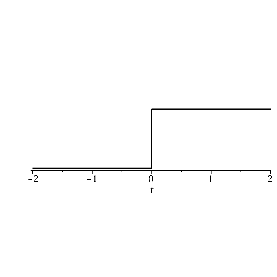

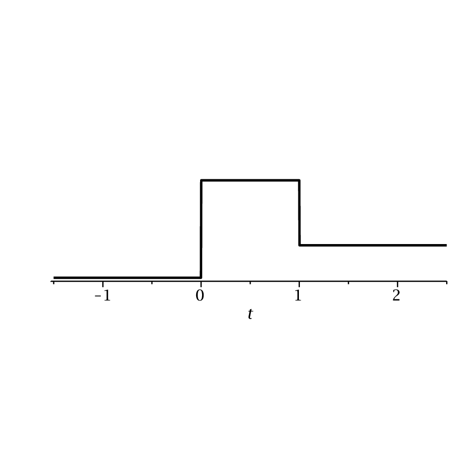

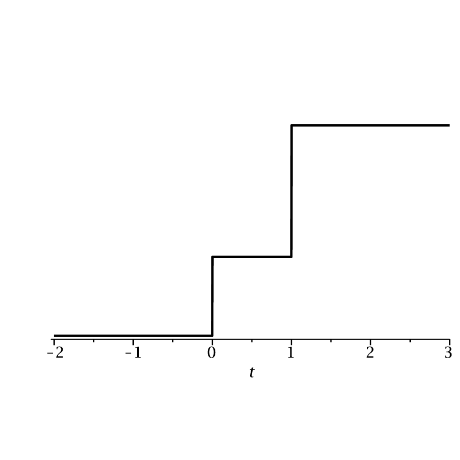

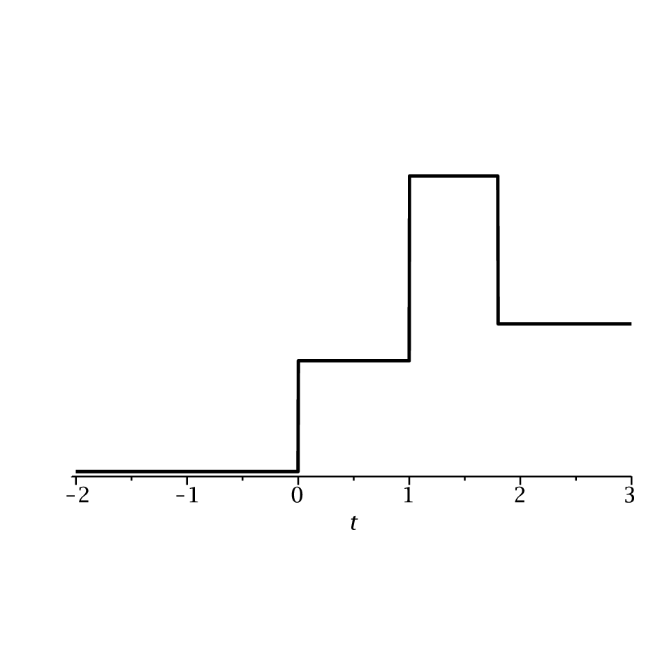

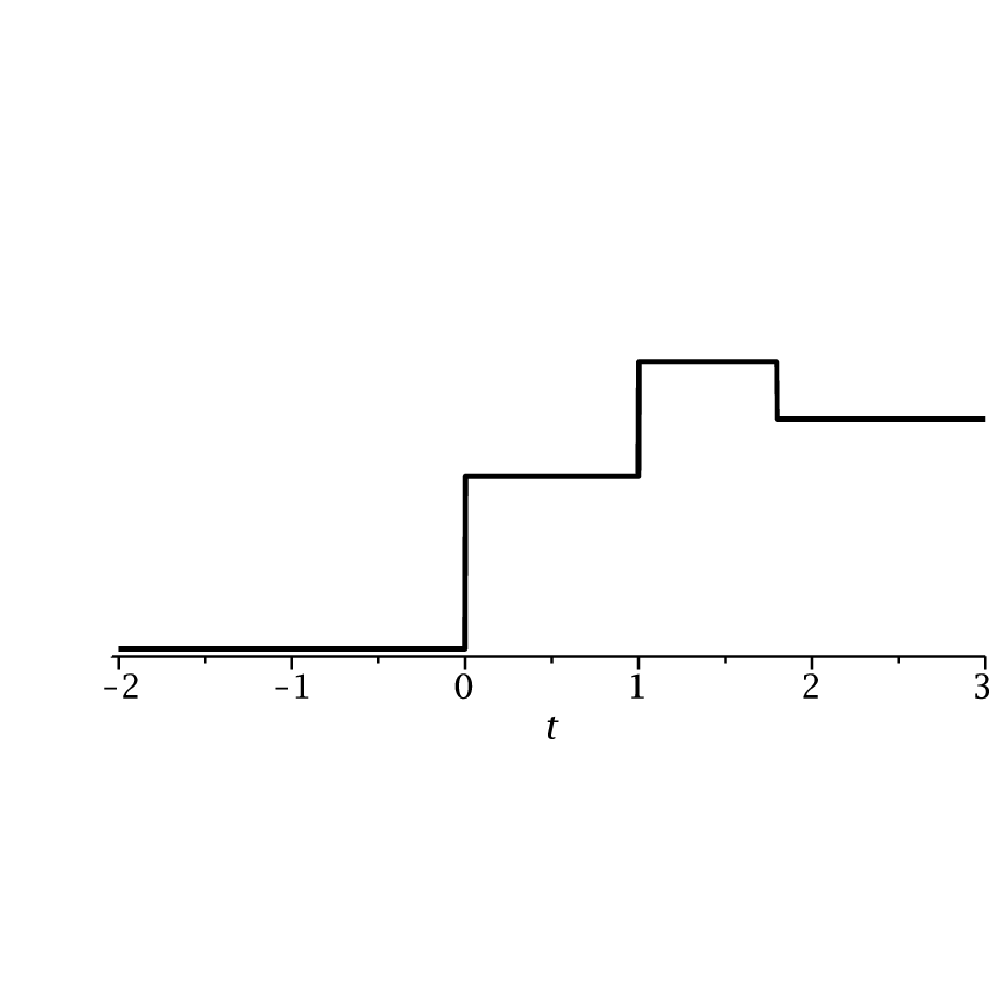

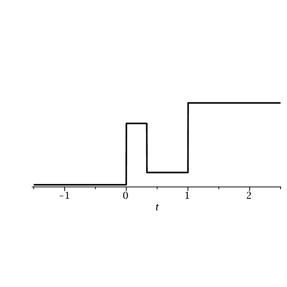

The six patterns each model a particular type of edge. Pattern
1 models an isolated step-edge, that is, if the intensity at the
boundary of the object changes at a single jump. Pattern 2 models a
thin object or an impulse, while Pattern 3 models a boundary where the
intensity changes at two isolated jumps. Pattern 4 and pattern 5 model
an object with boundary similar to Pattern 3, but where the intensity
decreases shortly after the initial intensity-changes. This occurs for
instance if there is a ’void’ within the object. If the object has a
’hole’ near the boundary one can model this with Pattern 6.
Pattern 4 and pattern 5 differ by the time-scale behavior of the
maxima-lines, fig.3(h,j). Given (or
) the point of transformation between the patterns are given
by (or ). or can be found by solving;
| (2) |
Fig.3 shows typical examples of the
patterns and their respective maximal-lines. Every pattern can after a
suitable normalization and translation be assumed to have an edge at
with intensity . Pattern 3-6 have (after rescaling) an
additional edge at with (positive) intensity , and pattern
2,4-6 have an edge of (negative) intensity at . The
six patterns have one (pattern 1), two (pattern 2,3) and three
(pattern 4-6) maxima-lines, in what follows denoted ,
and .
In fig.3 the six
patterns and characteristic examples of their maxima-lines are
displayed. As indicated in fig.3h, one can expect
that distance between mod-max is a weak criterion for pattern
4. Rather surprisingly this is also the case for pattern 3. Observe
that the maxima-lines of these ’simple’ patterns show a complexity
similar to those in medical ultrasound signals.
A
common factor of pattern 3-6 is that there exists a scale where the
maxima-line (pattern 3,4,6), (pattern 5) or
(pattern 6) first appears. This scale is found by
solving the equations;
| (3) |
The unique for which (3) has a solution is denoted . As it happens, the suggested time-scale filtering procedure is often most critical near .
3.3 Evaluation of the time-scale filtering procedure.
The purpose of the forthcoming analysis is to study for which patterns
(i.e. for which ) the time-scale filtering procedure
suggested in Sect.3.1 works. We also study the procedure for
different control-parameters .
Let as
before , and denote the maxima-lines
in the patterns from Sect.3.2 and fix two scales
and . We chose in this study , i.e. the scales
are dyadic distributed. In what follows let
be the decision-function corresponding to and defined in
Sect.3.1.
It is straightforward to see that the
procedure works for the first two patterns, hence we focus our
analysis on patterns . The decision-function
needs to fulfill one inequality for each
maxima-line. Namely; the decision-function connects two mod-max
and from the maxima-line if;
| (4) |
Similarly the mod-max and are connected if;
| (5) |
Note that for pattern 3 the inequalities (4) and (5) have to hold only for and respectively since does not exist. Finally, for pattern 4-6 the suggested procedure connects two mod-max from the maxima-line if;
| (6) |
Inequality (6) always holds for pattern 4-6 since
only if (since and ). We will therefore focus the
analysis on the inequalities (4) and (5).
For pattern 3,4,6 the decision-function successfully connects
any two mod-max if both inequalities (4)
and (5) hold for all scales such that
exists. Consequently (4) has to hold for every and (5) for all . For
pattern 5 both (4) and (5) have to hold
for all scales such that is well-defined. Thus
(4) has to hold for
every and (5) for all .
Comment: The preceding analysis of the
decision-function focuses on patterns with
values of typical for our specific application (locally
model medical ultrasound signals). Values of and/or
near the ’transformation-limit’ (value of where a
pattern transforms into another) will not be studied. In practice
one can
often consider such ’critical’ configurations by another pattern.
Pattern 3: First we consider the
decision-function and corresponding time-scale filtering procedure
with respect to pattern 3. Numerical analysis suggests that
the time-scale filtering procedure is most likely to fail at the
largest scale where both and exist. We can therefore
simplify the analysis by considering the left-hand-side (lhs.) of
(4) with , and lhs. of
(5) with , . Note that the
lhs. of (4) and (5) - denoted and
- are now functions depending only on . In
particular, if both and the suggested
procedure holds.


Fig.4 displays the graphs of respectively
and for given by (1) with
control-parameters (cyan,
yellow, blue, red, green). The dashed and dash-dotted lines correspond
to the ’limit cases’ resp. and
.
From fig.4a
one can see that along the maxima-line the decay-criterion
(dotted line) is optimal for connecting mod-max; if then (i.e. (4) holds) for all
. Along one need to have ,
fig.4b. On the contrary; if one considers the
distance-criterion (dash-dotted line) it suffices to have at fine scales, but needs to have at coarse
scales. Consequently one must have in order to
connect mod-max between any two scales and for pattern 3 if either or .
Combining distance and decay increase the -interval for
which the time-scale filtering procedure works, fig.4. If
e.g. is given by (1) with (yellow line) then it suffices to have to
connect mod-max between (any) two scales in pattern 3. If (blue line) then both and for all .


Pattern 4: For pattern 4 there are
three maxima-lines, , and . As
illustrated in fig.3h the edge at ’repels’
the maxima-lines corresponding to the edges at and . The result
is that the distance between and gets smaller, hence
weakening the distance-criterion for pattern 4.
For pattern
4 the time-scale filtering procedure successfully connect mod-max
across scales if both (4) and (5) holds. For this
purpose let denote the minimum of the lhs. of
(4) with respect to , , and , where
is given by (2) (recall that pattern 4 transforms into
pattern 5 for ). Similarly let denote
the minimum of the lhs. of (5) with , and . If both and
the procedure
successfully connects any two mod-max with respect to pattern 4.
The additional variables and make the analysis of
and more complicated for pattern 4-6 than for pattern
3. Rather than considering the graphs of and we study the
(level-curves of the) surfaces ,
. Numerical analysis indicates that both and
increase if: (i): the jump at location increases,
(ii): the jump at decreases, or (iii): the
distance from to increases. In particular, if
then for
all and , and similarly for .
As with pattern 3; different values of the control-parameter
’interpolates’ given by
(1) in between the ’limit’ cases and . Fig.5 displays the level-curves of the
surface with respect to given
by (1) with (note that the y-axis
differs in the figures). Fig.6 displays the
level-curves of for . Numerical studies indicate that if
, except possibly near critical values of
such as e.g. (which are
uninteresting to study for our purpose).
As expected;
increasing the influence of the decay-criterion increases the accuracy
of the time-scale filtering procedure for pattern 4. The following
table illustrates this for a few concrete values of and .
The table shows the maximal -interval such that the time-scale
filtering procedure works for some values of and ;
| A | ||||
|---|---|---|---|---|
As one can observe in the table, the reliability of the time-scale
filtering procedure increases with respect to pattern 4 if we increase
the influence of the decay-criterion.


Pattern 5:For pattern 5 the
situation is similar as with pattern 4. The edge at will - as
before - ’push’ the other maxima-lines away. However, since the ’long’
maxima-line now approaches (and not as for pattern 4,
fig.3(h,j)), we expect that the distance-criterion
will be strengthened.
Let as before denote
the minimum of the lhs. of (4) for and .
Given one can find by solving (2). Let
denote the minimum of the lhs. of (5) for
and .
Fig.7 and
fig.8 show some level-curves of the surfaces
for defined in
(1) with . Given the pair
in the -plane the point on the surface
represents the maximal value of such that the
procedure successfully connects mod-max along the maxima-line
for .
One may observe that the reliability of the
decision function increases if we increase
the weighting of the distance-criterion. Indeed; , for ’almost’ all if
or if is given
by (1) with . On the other hand, if
one can roughly say that one must have to ensure that both and .
Pattern 6: Fig.9 and
fig.10 show a few examples of the analysis of the
decision-function with respect to pattern 6. Similar to the
previous patterns let denote the minimum of the
lhs. of (4) wrt. and . Given one can find
by solving (2) (If the maxima-line at coarse
scales trifurcates). Let denote the minimum of the
lhs. of (5) wrt. , and .
Fig.9 and
fig.10 show some results of the analysis of pattern 6
with for and . If is close to either or one can in
practice model the signal as pattern 1, pattern 2 or pattern 3,
depending on mutual relations between and . For large
values of and the maxima-lines become unstable
making numerical analysis difficult.
The surfaces
represent the minimal
such that for all . Fig.9 shows some level-curves of the surface
for given by (1)
with . Fig.10 shows the some
level-curves of the surface for
given by (1) with . Numerical studies suggest that for
all , and if or ,
except possibly for .
One may observe
in fig.9 and fig.10 that increasing the
influence of the distance-criterion increases the reliability of the
scale-space filtering procedure for pattern 6. This is caused by the
edge at which ’pushes’ the other
maxima-lines away in different directions and hence strengthens the
distance-criterion. In addition, the edge at has negative
intensity which disrupts the decay-coefficient of the
wavelet transform, and hence the accuracy of the decay-criterion.


3.4 Summary and discussion of 1-D time-scale filtering procedure.
We have studied the
suggested time-scale filtering procedure from Sect.3.1 with
respect to the six model-patterns in Sect.3.2.
Connecting mod-max across time-scale plane for the first two
patterns is trivial. For the other patterns the overall accuracy of
the decision-function in general increases
if we use a suitable weighting between the distance- and
decay-criterion. For pattern 3 and pattern 4 the accuracy of the
decision-function benefits from increasing
the influence of the decay-criterion. For the last two patterns we saw
that increasing the influence of the distance-criterion increases the
accuracy of the time-scale filtering procedure. It is clear that one
should take specific features of the concrete signals into account
when defining the mutual weighting between distance- and
decay-criterion. When analyzing the medical ultrasound images in
Sect.5.3 we use .
In
Sect.5.1 we will evaluate the performance of the
proposed time-scale filtering procedure with respect to medical
ultrasound signals.
The results from the previous sections
are useful also for more complicated signals. For instance the signal
is locally similar to pattern 3 near
the point and pattern 4 near the point . Due to fast decay of
the wavelet the maxima-lines of the ’local’ patterns in
and their exact equivalent are practically identical for
. It makes little sense to analyze the signal at
scales for the purpose of edge-detection. Our analysis of
actual medical ultrasound signals indicates that such signals often
are composed of (distinct) patterns in this manner as illustrated in
fig.2.
Real medical ultrasound signals are of
course ’smooth’. The corresponding edges can be modeled by smoothed
versions of the ’ideal’ patterns in Sect.3.2. If
is any of the ideal patterns say, then we can model the smoothed
patterns as where , is
the Gaussian smoothing kernel.
With some natural
modifications the suggested time-scale filtering procedure applies to
the smoothed patterns as well. We need to use denser (i.e. non-dyadic)
scales; more precisely we need to choose such that
. If we in
addition change to in the expression for the decay-criterion
, the results from Sect.3.3 apply directly
(i.e. with
the same ).
3.5 Decision-function and space-scale filtering procedure for 2-D signals.
We turn the attention towards a space-scale filtering procedure for
connecting mod-max across the space-scale plane of 2-D
signals. In images mod-max are chained together to form
boundary-curves corresponding to boundaries of objects, and
the natural space-scale plane object is the
maxima-surface. The behavior of a maxima-surface is more
subtle than for a maxima-line. For instance one can not assume that a
maxima-surface does not branch. The target with the space-scale
filtering procedure is to decide which mod-max propagate toward each
of the boundary-curves at the finest scale.
The suggested
decision-function for 2-D signals is - with some natural modifications
- similar to the 1-D decision-function defined in Sect.3.1. Let
and be two scales , and let and be
two mod-max. We define the decision-function as;
where;
is the direction of the wavelet transform at the mod-max , and is given by
The essence of the space-scale filtering procedure is - as in 1-D - to
connect mod-max which maximize .
In
particular, if one consider 2-D patterns obtained by a tensor product
of the 1-D patterns, then the analysis in Sect.3.3 extends
to the 2-D procedure.
Given two scales the
procedure requires that for each one has to
compute for every . One can reduce the
computational efforts by computing only for
within a given
distance ( should suffice if we use dyadic scales) of .
In the next section we will see that for our purpose it is
sufficient to compute for only a few mod-max at scale
as well. By using these simplification one will effectively reduce the
computational complexity of the space-scale filtering procedure for
images.
4 Edge-detection.
The uncertainty-principle states that in a noisy signal there
exists no single scale such that one can detect and simultaneously
localize only the significant edges, [3]. However, by using
the maxima-lines one can turn the uncertainty-principle into our
advantage. At coarse scale one can detect the significant edges in the
signal, and at fine scales one can localize them. Since maxima-lines
connect coarse- and fine-scale information one can effectively improve
edge-detection in noisy signals.
In this section we discuss
a multi-scale wavelet-based edge-detection scheme. The method is based
on the suggested time-scale filtering procedure and a perceptual
criteria similar to that in [6]. This approach has shown
promising results for detecting and localizing (low-contrast) edges in
medical images.
4.1 1-D edge-detection.
Assume that the wavelet transform is computed at scales for , and let denote the mod-max at the finest scale . For a mod-max let denote the maxima-line which contains . To each assign the number;
If need be one can introduce a weight-function in the expression for , for instance to favor fine/coarse scale information. The final step of the edge-detector is to decide a threshold and find the mod-max such that . These mod-max are used to represent the significant edges in the signal.
4.2 2-D edge-detection
Assume that the wavelet transform is computed at scales for and let denote the boundary-curves at scale .
To each maxima-curve we assign the following quantity;
| (7) |
where denotes the average-function. The final
step of the edge-detection is to identify the curves such that
, where is a threshold. These
boundary-curves is used to represent the boundaries of significant
edges in the image.
The quantity reduces the influence of a few false connections made by the
space-scale filtering procedure along a boundary-curve . Such
false connections can occur for some ’critical’ patterns (e.g. in pattern 3).
As mentioned in Sect.3.5
on can save computational efforts by reducing the number of ’s for
which one has to compute . Further reduction can be achieved
by computing the average in (7) from only a ’few’
randomly selected maxima-lines from each maxima-curve
. Experiments indicate that this simplification has little
influence on the values of .
5 Experiments and results.
We test the edge-detector on both phantom and actual
medical ultrasound signals. By studying the algorithm on
phantom-signals we compare the Figure of Merit [19] with the
Canny edge-detector. The visual performance of the edge-detector is
analyzed with respect to medical ultrasound signals. This
analysis focuses on some well-known problem features of
medical ultrasound images; such as low-contrast edges and speckle-noise.
Before studying the edge-detection algorithm we analyze the
reliability of the suggested time-scale filtering procedure on actual
signals. The main question is whether the results from
Sect.3 also apply to actual medical ultrasound signals.
5.1 Accuracy of time-scale filtering procedure on medical ultrasound signals.
To quantitatively
evaluate the performance of the suggested time-scale filtering
procedure from Sect.3.1 we compare the output of the procedure
with the exact maxima-lines of the wavelet transform. Assuming that
the procedure connects the mod-max to and say, then we will study if . The
test-signals used to evaluate the procedure are 1-D cross-sections of
medical ultrasound images.
In the analysis we study the
probability of a false connection, and between which scales an error
is most likely to occur. For the purpose of edge-detection the
severity of a false connection increases at coarse scales. We also
study the average displacement (in pixels) of a mod-max caused by a
false connection. If this number is small it indicates that an error
has little influence on the visual output of the edge-detector.
In the experiments we use scales . The control-parameter is chosen as 11
1
Note that in the analysis of the patterns in
Sect.3 we had in the expression for
in (1). In particular . Since we are using scales to
analyze actual medical ultrasound signals we will necessarily have
. This causes that a large
favors decay-criteria and a small favors the
distance-criteria. I.e. in the preceding section
’corresponds’ to in this section, and visa verse for
.. To obtain the actual maxima-lines we use the
edge-focusing algorithm [4].
The results of the
quantitative analysis of the time-scale filtering procedure is
displayed in Tab.1-3. Each column
represents the average performance of the procedure applied to every
horizontal cross-section in the corresponding image. The images are
displayed in fig.12(a,b,c) and fig.11b.
| Signal: | Tumor | Blood - vessel | Liver | phantom |
| False connections : | 4.8 | 4.7 | 6.2 | 4.2 |
| Spatial error in pixels: | 12.4 (2.5) | 12.9 (2.5) | 12.2 (2.8) | 20.3 (7.4) |
| False connections between scale and : | 2.5 | 4.4 | 8.5 | 4.2 |
| False connections between scale and : | 5.4 | 5.2 | 9.0 | 8.0 |
| False connections between scale and : | 6.2 | 5.7 | 8.2 | 5.0 |
| False connections between scale and : | 4.8 | 4.5 | 6.0 | 1.7 |
| Signal: | Tumor | Blood - vessel | Liver | phantom |
| False connections : | 4.0 | 4.2 | 4.8 | 3.8 |
| Spatial error in pixels: | 11.5 (2.2) | 13.2 (2.6) | 12.6 (2.9) | 19.2 (7.0) |
| False connections between scale and : | 1.9 | 4.3 | 8.6 | 3.3 |
| False connections between scale and : | 4.3 | 5.3 | 7.9 | 8.0 |
| False connections between scale and : | 5.2 | 4.8 | 5.4 | 4.1 |
| False connections between scale and : | 4.1 | 3.9 | 4.7 | 1.6 |
| Signal: | Tumor | Blood - vessel | Liver | phantom |
| False connections : | 3.9 | 4.0 | 4.6 | 3.7 |
| Spatial error in pixels: | 11.7 (2.3) | 13.5 (2.6) | 13.3 (3.1) | 19.3 (7.0) |
| False connections between scale and : | 1.9 | 4.3 | 8.6 | 3.3 |
| False connections between scale and : | 4.4 | 5.3 | 7.8 | 7.8 |
| False connections between scale and : | 5.0 | 4.5 | 5.2 | 4.0 |
| False connections between scale and : | 4.0 | 3.7 | 4.5 | 1.6 |
The analysis of pattern 6 in Sect.3.3 showed that the accuracy of the suggested time-scale filtering procedure increases as increases from to . Speckle noise can often locally be modeled as pattern 6 (with and ). Hence we expect to observe a similar increase in accuracy for actual medical ultrasound signals. In Tab.1-3 one can indeed observe such increase of the accuracy of the procedure on medical ultrasound signals (recall that in this analysis corresponds to in the analysis in Sect.3, etc). A closer inspection indicates that false connections in between maxima-lines corresponding to speckle-noise is the typical problem for the time-scale filtering procedure on ultrasound signal. Since speckle-noise contains information which is unwanted from an edge-detection viewpoint, such false connections will only be a minor problem.
5.2 Results of edge-detection on phantom ultrasound images.
To study the performance of the edge-detection algorithm
suggested in Sect.4.2 we compare it with the well-known
Canny edge-detector. We believe that comparing the Canny edge-detector
with ours demonstrates some differences between multi-scale and
single-scale wavelet-based edge-detection.
For the Canny
edge-detector with hysteria we have used thresholds and . The scale is chosen equal to the
finest scale used by our algorithm.
To quantitatively
analyze the edge-detectors we study the phantom medical ultrasound
signals shown in fig.11.


The image in fig.11(a) shows the noise-free version,
and fig.11(b,c) shows the images with various
speckle-noise. The phantom images are generated by using a region
image as a variance field for the diffuse scattering. The images are
made by convolving the ideal image with a parametric point-spread
function and adding white Gaussian noise, and are discussed in details
in [20, 21]22
2
The images are kindly provided by SINTEF
MedTech. The author thanks T. Langø for his assistance..
We use the well-known Figure of Merit (FOM)[19] to
quantitatively evaluate the edge-detection algorithms. The FOM is the
number defined as;
where and are the number of resp. true and detected edges,
and is the minimal distance from a detected to a true
edge. is a constant used to penalize displaced mod-max. To be
consistent with others we use [8, 22]. The
should ideally be close to .
The values of
the Figure of Merit of the two edge-detectors are displayed in
tab.4 - 5.
| Signal: | proposed edge-detector | Canny |
|---|---|---|
| phantom 1: | 0.56 | 0.53 |
| phantom 2: | 0.54 | 0.47 |
| Signal: | proposed edge-detector | Canny |
|---|---|---|
| phantom 1: | 0.54 | 0.53 |
| phantom 2: | 0.53 | 0.51 |
5.3 Result of edge-detection on real ultrasound images.
In this section we discuss the results of the suggested
edge-detection algorithm on real signals. For this purpose we study
the edges detected by the algorithm in several actual medical
ultrasound images. The goal is to study if the algorithm detects the
significant edges in the images without including irrelevant
information such as noise. In addition we
discuss how one can obtain a threshold as well as the computational
complexity of the
algorithm.


Fig.12 shows the ultrasound images which are
discussed in this section. Each image contains some typical features
of medical ultrasound images which cause difficulties for
edge-detection.
Fig.12(a),
Brain-tumor image: The interesting edges are the outer boundary of
the tumor and the cortex (white ’horizontal’ object to the south-west
of the tumor). The voids within the tumor are mainly interesting in
order to study how the edge-detector represents fine details.
Fig.12(b), Liver image: The interesting
edge is the boundary of the liver. The boundary is the horizontal line
in the upper third in the image. This image interesting to study
because of the low CNR of the boundary.
Fig.12(c), Blood-vessel image: In this image we
want to detect the boundary of the blood-vessel. Some parts of the
boundary of the blood-vessel have low contrast making them difficult
to detect. This problem is typical for ultrasound images of
blood-vessels.


Edge-detection and noise-removal:
Fig.13(a,b,c) shows some results of our edge-detection
algorithm applied to the images in fig.12. Most of the
significant edges which we would like to detect are present in the
representations. One may also observe, in particular in
fig.13(a,c), that the representations contain few edges
which can be ascribed to noise. The representations in
fig.13 show promising results for detecting low contrast
edges and fine detail edges. However, the boundary-curves of such
edges are vulnerable to fragmenting (which make them difficult to
detect). This phenomenon occurs for instance underneath the tumor (low
contrast) and to some degree inside the tumor (fine details). The
fragmenting - in particular for low-contrast edges - appears to
increase due to speckle-noise. One can reduce this problem by
connecting fragmented boundary-curves (e.g. by using coarse scale
information as suggested in [6]). Preliminary studies have
shown that using this as a complimentary tool improves edge-detection
of low-contrast and fine detail edges. We use no synthesizing of the
boundary-curves in this study.
Fig.13(d,e,f)
shows the result obtained by using the Canny edge-detector (with
hysteria). The scales is chosen equal the finest scale used by our
algorithm. One can observe that the edge-detector scheme studied in
Sect.4.2 in general yields better representations of
the significant edges in the images, and includes less noise.
Threshold: The edge-detector assigns to each
boundary-curve a value representing both its length and
value of wavelet transform in both time- and scale-space. Values of
corresponding to noise will therefore be concentrated at low
values, while those corresponding to edges will be distributed
discretely at high values. The result is that there is often a
separation between values of corresponding to noise and edges. A
similar phenomenon was observed in [6]. In addition, since
values of corresponding to significant edges are often distributed
discretely it is possible to find representations which are
perceptually optimal.
Computational complexity: The
computational complexity of the edge-filtering procedure in
Sect.4.2 is negligible. In what follows we focus on the
computational complexity of computing the wavelet transform and the
space-scale filtering procedure from Sect.3.5.
To
reduce the computational complexity of the space-scale filtering
procedure we use the tricks discussed in Sect.3.5 and
Sect.4.2. In other words we find the maxima-lines of
only a few randomly selected mod-max along each boundary-curve, and
use a sliding window (of size to decide candidate connections at the next finer
scale. We use the fast Fourier-transform to compute the wavelet
transform.
The space-scale filtering procedure has been
implemented in MATLAB version 7.9.0 (R2009b) on a laptop with a
Pentium 3 (2 GHz) processor. Tested on a image the
total processing time is seconds if we find the maxima-lines of
of the mod-max. If we find only randomly selected
maxima-lines the total processing time is sec.
Computationally both computing the wavelet transform at different
scales and connecting mod-max across scales is well-suited for
parallel-computing. It is expected that this should allow us to
further reduce the total processing-time of the scale-space filtering
procedure.
6 Conclusion
We suggest a fast multi-scale edge-detection algorithm for medical
ultrasound signals. The edge-detector is based on the continuous
wavelet transform, and takes advantage of the behavior of maxima-lines
in the space-scale plane. Our algorithm shows promising results for
detecting the significant edges in medical ultrasound signals.
The key-point of the edge-detection scheme is a fast
space-scale filtering procedure for medical ultrasound signals. The
procedure is designed to accommodate a set of patterns modeling
intensity-changes which are typical in such signals. This allow us to
manage and reduce the ambiguity introduced when using the multi-scale
wavelet transform to detect edges in a medical ultrasound signal. The
space-scale filtering procedure connects mod-max which belong to the
same maxima-line by computing the wavelet transform at only a sparse
set of scales. For our medical ultrasound signals we typically need to
compute the wavelet transform at the four scales . In the popular Edge-focusing algorithm [4] one
computes the wavelet transform at a linear set of scales () to trace mod-max in the space-scale plane. Our proposed
space-scale filtering procedure will therefore considerably reduce the
computational efforts needed to decide which mod-max belong to the
same maxima-line.
Based on the space-scale filtering
procedure we study a novel edge-detection algorithm for medical
ultrasound signals. The edge-detector assigns to each candidate edge a
value representing the behavior of its corresponding maxima-line in
the space-scale plane. Experimental results indicate that the
edge-detector finds both high- and low-contrast edges in medical
ultrasound images and yet disregards noise. Compared to the Canny
edge-detector we observe that our algorithm finds the significant
edges, and includes less redundant information such as noise. Our
study has showed that one can construct multi-scale edge-detection
algorithm for medical ultrasound signals which meets the demand of
speed, but not on the expense of reliability.
We also expect
that using multi-scale information opens new possibilities for further
improvements of edge-detection in medical ultrasound images. One
possibility is to dynamically choose the finest scale based on local
automatic scale selection as described in e.g. [16].
Acknowledgment
The author would first of all like to thank his supervisor Prof. Yurii
Lyubarskii for the support and guidance during the work.
The
author would also like to thank Dr. Jianhua Yao (National Institue of
Health) for useful discussions.
The author would like to
thank SINTEF Medical Technology for providing medical ultrasound
images obtained through clinical studies at St. Olavs Hospital,
Trondheim, Norway.
References
- [1] I. Daubechies, Ten lectures on wavelets, Society for Industrial and Applied Mathematics, Philadelphia, PA, USA, 1992.
- [2] S. Mallat, A wavelet tour of signal processing, 2nd Edition, Academic Press, 1998.
- [3] J. Canny, A computational approach to edge detection, IEEE transactions of pattern analysis and machine intelligence PAMI-8 (6) (1986) 679–698.
- [4] F. Bergholm, Edge focusing, IEEE transactions of pattern analysis and machine intelligence PAMI-9 (6) (1987) 726–741.
- [5] A. P. Witkin, Scale-space filtering: A new approach to multi-scale description, in: Proc. IEEE International Conference on Acoustics, Speech, and Signal Processing (ICASSP), Vol. 9, IEEE, San Diego, CA, 1984, pp. 150–153.
- [6] J. Lu, J. D. Weaver, J. Dennis M. Healy, Y. Xu, Noise reduction with a multiscale edge representation and perceptual criteria, in: in Proceedings of IEEE-SP International Symposium on Time-Frequency and TimeScale Analysis, 1992, pp. 555–558.
- [7] B. Sumengen, B. S. Manjunath, Multi-scale edge detection and image segmentation, in: European Signal Processing Conference (EUSIPCO), 2005.
- [8] Y. Yue, M. M. Croitoru, A. Bidani, J. B. Zwischenberger, J. W. Clark, Nonlinear multiscale wavelet diffusion for speckle suppression and edge enhancement in ultrasound images, IEEE transactions on medical imaging 25 (3) (2006) 297–311.
- [9] L. Zhang, P. Bao, Edge detection by scale multiplication in wavelet domain, Pattern Recogn. Lett. 23 (2002) 1771–1784.
- [10] M. Shah, A. Sood, R. Jain, Pulse and staircase edge models, Comput. Vision Graph. Image Process. 34 (1986) 321–343.
- [11] Y. Lu, R. C. Jain, Behaviour of edges in scale space, IEEE transactions of pattern analysis and machine intelligence 11 (4) (1989) 337–356.
- [12] C. Ducottet, T. Fournel, C. Barat, Scale-adaptive detection and local characterization of edges based on wavelet transform, Signal Process. 84 (2004) 2115–2137.
- [13] D. Ziou, S. Tabbone, Edge detection techniques - an overview, International Journal of Pattern Recognition and Image Analysis 8 (1998) 537–559.
- [14] S. Mallat, S. Zhong, Characterization of signals from multiscale edges, IEEE transactions on pattern analysis and machine intelligence 14 (7) (1992) 710–732.
- [15] S. Mallat, W. L. Hwang, Singularity detection and processing with wavelets, IEEE transactions on information theory 38 (2) (1992) 617–643.
- [16] T. Lindeberg, Edge detection and ridge detection with automatic scale selection, International Journal of Computer Vision 30 (2) (1998) 117–156.
- [17] F. Guo, Y. Yang, B. Chen, L. Guo, A novel multi-scale edge detection technique based on wavelet analysis with application in multiphase flows, Powder Technology 202 (1-3) (2010) 171–177.
- [18] R. Zhang, W. Ouyang, W.-K. Cham, Image multi-scale edge detection using 3-d hidden markov model based on the non-decimated wavelet, in: Image Processing (ICIP), 2009 16th IEEE International Conference on, 2009, pp. 2173 –2176.
- [19] W. K. Pratt, Digital image processing, 2nd Edition, John Wiley & Sons, Inc., 1991.
- [20] O. Husby, T. Lie, T. Langø, J. Hokland, H. Rue, Bayesian 2-d deconvolution: A model for diffuse ultrasound scattering, IEEE transactions on ultrasonics, ferroelectrics, and frequency control 48 (1) (2001) 121–130.
- [21] T. Langø, T. Lie, O. Husby, J. Hokland, Bayesian 2-d deconvolution: Effect of using spatially invariant ultrasound point spread functions, IEEE transactions on ultrasonics, ferroelectrics, and frequency control 48 (1) (2001) 131–141.
- [22] S. Yi, D. Labate, G. R. Easley, H. Krim, A shearlet approach to edge analysis and detection, IEEE Transactions on Image Processing 18 (5) (2009) 929–941.