Normalized graph Laplacians for directed graphsThanks: 2010 Mathematics Subject Classification. 05C20, 05C22, 05C50

Frank Bauer Address: Max Planck Institute for Mathematics in the Sciences
Leipzig 04103, Germany. Email address: Frank.Bauer@mis.mpg.de

Abstract.

We consider the normalized Laplace operator for directed graphs with positive and negative edge weights. This generalization of the normalized Laplace operator for undirected graphs is used to characterize directed acyclic graphs. Moreover, we identify certain structural properties of the underlying graph with extremal eigenvalues of the normalized Laplace operator. We prove comparison theorems that establish a relationship between the eigenvalues of directed graphs and certain undirected graphs. This relationship is used to derive eigenvalue estimates for directed graphs. Finally we introduce the concept of neighborhood graphs for directed graphs and use it to obtain further eigenvalue estimates.

Key words and phrases:

directed graphs, normalized graph Laplace operator, eigenvalues, directed acyclic graphs, neighborhood graph

To appear in: Linear Algebra and its Applications

1. Introduction

For undirected graphs with nonnegative weights, the normalized graph Laplace operator $\Delta$ is a well studied object, see e. g. the monograph [8]. In addition to its mathematical importance, the spectrum of the normalized Laplace operator has various applications in chemistry and physics. However, it is not always sufficient to study the normalized Laplace operator for undirected graphs with nonnegative weights. In many biological applications, one naturally has to consider directed graphs with positive and negative weights [3]. For instance, in a neuronal network only the presynaptic neuron influences the postsynaptic one, but not vice versa. Furthermore, the synapses can be of inhibitory or excitatory type. Inhibitory and excitatory synapses enhance or suppress, respectively, the activity of the postsynaptic neuron and thus the directionality of the synapses and the existence of excitatory and inhibitory synapses crucially influence the dynamics in neuronal networks [3]. Hence, a realistic model of a neuronal network has to be a directed graph with positive and negative weights in which the neurons correspond to the vertices and the excitatory and inhibitory synaptic connections are modelled by directed edges with positive and negative weights, respectively.

In contrast to undirected graphs not much is known about normalized Laplace operators for directed graphs. In [9] Chung studied a normalized Laplace operator for strongly connected directed graphs with nonnegative weights. This Laplace operator is defined as a self-adjoint operator using the transition probability operator and the Perron vector^*^* * A similar construction is used in [25] to study the algebraic connectivity of the Laplace operator $L=D-W$ defined on directed graphs.. For our purposes, however, this definition of the normalized Laplace operator is not suitable since by the above considerations we are particularly interested in graphs that are neither strongly connected nor have nonnegative weights. In this article, we define a novel normalized Laplace operator that can in particular be defined for directed graphs that are neither strongly connected nor have nonnegative weights. In contrast to Chung’s normalized Laplace operator our normalized Laplace operator is in general neither self-adjoint nor nonnegative. Moreover, our definition of the normalized Laplace operator is motivated by the observation that it has already found applications in the field of complex networks, see [2, 3].

The paper is organized as follows. In Section $2$ we define the normalized Laplace operator for directed graphs and in Section $3$ and Section $4$ we derive its basic spectral properties. In Section $5$ we characterize directed acyclic graphs by means of their spectrum. Extremal eigenvalues of the Laplace operator are studied in Section $6$ and Section $7$ . In Section $8$ we prove several eigenvalues estimates for the normalized Laplace operator. Finally in Section $9$ we introduce the concept of neighborhood graphs and use it to derive further eigenvalue estimates.

2. Preliminaries

Unless stated otherwise, we consider finite simple loopless graphs. Let $\Gamma=(V,E,w)$ be a weighted directed graph on $n$ vertices where $V$ denotes the vertex set, $E$ denotes the edge set, and $w:V\times V\rightarrow{\mathbb{R}}$ is the associated weight function of the graph. For a directed edge $e=(i,j)\in E$ , we say that there is an edge from $i$ to $j$ . The weight of $e=(i,j)$ is given by $w_{ji}$ ^†^† † We use this convention instead of denoting the weight of the edge $e=(i,j)$ by $w_{ij}$ , since it is more appropriate if one studies dynamical systems defined on graphs, see for example [2]. and we use the convention that $w_{ji}=0$ if and only if $e=(i,j)\notin E$ . The graph $\Gamma=(V,E,w)$ is an undirected weighted graph if the associated weight function $w$ is symmetric, i.e. satisfies $w_{ij}=w_{ji}$ for all $i$ and $j$ . Furthermore, $\Gamma$ is a graph with non-negative weights if the associated weight function $w$ satisfies $w_{ij}\geq 0$ for all $i$ and $j$ . For ease of notation, let $\mathbb{G}$ denote the class of weighted directed graphs $\Gamma$ . Furthermore, let $\mathbb{G}^{\mathrm{u}}$ , $\mathbb{G}^{+}$ and $\mathbb{G}^{\mathrm{u}+}$ denote the class of weighted undirected graphs, the class of weighted directed graphs with non-negative weights and the class of weighted undirected graphs with non-negative weights, respectively. The in-degree and the out-degree of vertex $i$ are given by $d_{i}^{\mathrm{in}}:=\sum_{j}w_{ij}$ and $d_{i}^{\mathrm{out}}:=\sum_{j}w_{ji}$ , respectively. A graph is said to be balanced if $d_{i}^{\mathrm{in}}=d_{i}^{\mathrm{out}}$ for all $i\in V$ . Since every undirected graph is balanced, the two notions coincide for undirected graphs. Thus, we simply refer to the degree $d_{i}$ of an undirected graph. A graph $\Gamma$ is said to have a spanning tree if there exists a vertex from which all other vertices can be reached following directed edges. A directed graph $\Gamma$ is weakly connected if replacing all of its directed edges with undirected edges produces a connected (undirected) graph. A directed graph $\Gamma$ is strongly connected if for any pair of distinct vertices $i$ and $j$ there exists a path from $i$ to $j$ and a path from $j$ to $i$ . An undirected graph is weakly connected if and only if it is strongly connected. Hence, we do not distinguish between weakly and strongly connected undirected graphs. We simply say that the undirected graph is connected if it is weakly (strongly) connected.

Definition 2.1.

Let $C(V)$ denote the space of complex valued functions on $V$ . The normalized graph Laplace operator for directed graphs $\Gamma\in\mathbb{G}$ is defined as

\Delta:C(V)\rightarrow C(V),

\displaystyle\Delta v(i)=\left\{\begin{array}[]{c l}v(i)-\frac{1}{d^{\mathrm{in}}_{i}}\sum_{j}w_{ij}v(j)&\mbox{if }d^{\mathrm{in}}_{i}\neq 0.\\ 0&\mbox{else}.\end{array}\right.

If $d^{\mathrm{in}}_{i}\neq 0$ for all $i\in V$ , then $\Delta$ is given by

\Delta=I-D^{-1}W,

where $D:C(V)\to C(V)$ is the multiplication operator defined by

(4)

Dv(i)=d_{i}^{\mathrm{in}}v(i)

and $W:C(V)\to C(V)$ is the weighted adjacency operator

Wv(i)=\sum_{j\in V}w_{ij}v(j).

When restricted to undirected graphs with nonnegative weights, Definition 2.1 reduces to the well-known definition of the normalized Laplace operator for undirected graphs with nonnegative weights, c.f.[19].

The choice of normalizing by the in-degree is to some extend arbitrary. One could also consider the operator

\overline{\Delta}:C(V)\rightarrow C(V),

\displaystyle\overline{\Delta}v(i)=\left\{\begin{array}[]{c l}v(i)-\frac{1}{d^{\mathrm{out}}_{i}}\sum_{j}w_{ji}v(j)&\mbox{if }d^{\mathrm{out}}_{i}\neq 0.\\ 0&\mbox{else}.\end{array}\right.

Note however, that both operators $\Delta$ and $\overline{\Delta}$ are equivalent to each other in the sense that $\Delta(\Gamma)=\overline{\Delta}(\overline{\Gamma})$ , where $\overline{\Gamma}$ is the graph that is obtained from $\Gamma$ by reversing all edges.

Since we consider a normalized graph Laplace operator, i. e. we normalize the edge weights w.r.t. the in-degree, vertices with zero in-degree are of particular interest and need a special treatment. We define the following:

Definition 2.2.

We say that vertex $i$ is in-isolated or simply isolated if $w_{ij}=0$ for all $j\in V$ . Similarly, vertex $i$ is said to be in-quasi-isolated or simply quasi-isolated if $d^{\mathrm{in}}_{i}=\sum_{j}w_{ij}=0$ .

Note that every isolated vertex is quasi-isolated but not vice versa. These definitions can be extended to induced subgraphs:

Definition 2.3.

Let $\Gamma=(V,E,w)\in\mathbb{G}$ be a graph and $\Gamma^{\prime}=(V^{\prime},E^{\prime},w^{\prime})$ be an induced subgraph of $\Gamma$ , i.e. $V^{\prime}\subseteq V$ , $E^{\prime}=E\cap(V^{\prime}\times V^{\prime})\subseteq E$ , and $w^{\prime}:V^{\prime}\times V^{\prime}\rightarrow\mathds{R}$ , $w^{\prime}:=w|_{E^{\prime}}$ . We say that $\Gamma^{\prime}$ is isolated if $w_{ij}=0$ for all $i\in V^{\prime}$ and $j\notin V^{\prime}$ . Similarly, $\Gamma^{\prime}$ is said to be quasi-isolated if $\sum_{j\in V\setminus V^{\prime}}w_{ij}=0$ for all $i\in V^{\prime}$ .

We do not exclude the case where $V^{\prime}=V$ . Thus, in particular, every graph $\Gamma$ is isolated.

It is useful to introduce the reduced Laplace operator $\Delta_{R}$ .

Definition 2.4.

Let $V_{R}\subseteq V$ be the subset of all vertices that are not quasi-isolated. The reduced Laplace operator $\Delta_{R}:C(V_{R})\to C(V_{R})$ is defined as

(8)

\Delta_{R}v(i)=v(i)-\frac{1}{d_{i}^{\mathrm{in}}}\sum_{j\in V_{R}}w_{ij}v(j)\quad i\in V_{R},

where $d_{i}^{\mathrm{in}}$ is the in-degree of vertex $i$ in $\Gamma$ .

As above $\Delta_{R}$ can be written in the form $\Delta_{R}=I_{R}-D_{R}^{-1}W_{R}$ where $I_{R}$ is the identity operator on $V_{R}$ .

It is easy to see that the spectrum of $\Delta$ consists of the eigenvalues of $\Delta_{R}$ and $|V\setminus V_{R}|$ times the eigenvalue $0$ , i. e.

(9)

\mathrm{spec}(\Delta)=(|V\setminus V_{R}|\mbox{ times the eigenvalue }0)\cup\mathrm{spec}(\Delta_{R}).

We remark here that $\Delta_{R}$ can be considered as a Dirichlet Laplace operator. The Dirichlet Laplace operator for directed graphs is defined as in the case of undirected graphs, see e. g. [16]. Let $\Omega\subseteq V$ and denote by $C(\Omega)$ the space of complex valued functions $v:\Omega\rightarrow\mathds{C}$ . The Dirichlet Laplace operator $\Delta_{\Omega}$ on $C(\Omega)$ is defined as follows: First extend $v$ to the whole of $V$ by setting $v=0$ outside $\Omega$ and then

\Delta_{\Omega}v=(\Delta v)|_{\Omega},

i. e. for any $i\in\Omega$ we have

\Delta_{\Omega}v(i)=v(i)-\frac{1}{d^{\mathrm{in}}_{i}}\sum_{j\in V}w_{ij}v(j)=v(i)-\frac{1}{d^{\mathrm{in}}_{i}}\sum_{j\in\Omega}w_{ij}v(j)

since $v(j)=0$ for all $j\in V\setminus\Omega$ . Hence, $\Delta_{R}=\Delta_{\Omega}$ if we set $\Omega=V_{R}$ .

As already mentioned in the introduction, we are particularly interested in graphs that are not strongly connected. However, every graph that is not strongly connected can uniquely be decomposed into its strongly connected components [6]. Using this decomposition, the Laplace operator $\Delta$ can be represented in the Frobenius normal form [6], i. e. either $\Gamma$ is strongly connected or there exists an integer $z>1$ s.t.

(10)

\Delta=\left(\begin{array}[]{cccccc}\Delta_{1}&\Delta_{12}&...&\Delta_{1z}&\\ 0&\Delta_{2}&...&\Delta_{2z}\\ \vdots&\vdots&\ddots&\vdots\\ 0&0&...&\Delta_{z}\end{array}\right),

where $\Delta_{1},\ldots\Delta_{z}$ are square matrices corresponding to the strongly connected components $\Gamma_{1},\ldots,\Gamma_{z}$ of $\Gamma$ . In the following, the vertex set of $\Gamma_{k}$ is denoted by $V_{k}$ . Then the off-diagonal elements of $\Delta_{k}$ are of the form $\frac{w_{ij}}{d^{\mathrm{in}}_{i}}$ for all $i,j\in V_{k}$ if $d^{\mathrm{in}}_{i}\neq 0$ and zero otherwise and the diagonal elements are either zero (if the in-degree of the corresponding vertex is equal to zero) or one (if the in-degree of the corresponding vertex is nonzero). If $V_{k}$ does not contain a quasi-isolated vertex, then $\Delta_{k}$ is irreducible. Furthermore, the submatrices $\Delta_{kl}$ , $1\leq k<l\leq z$ are determined by the connectivity structure between different strongly connected components. For example, $\Delta_{kl}$ contains all elements of the form $\frac{w_{ij}}{d^{\mathrm{in}}_{i}}$ for all $i\in V_{k}$ and all $j\in V_{l}$ . A simple consequence of (10) is that

(11)

\mathrm{spec}(\Delta)=\bigcup_{i=1}^{z}\mathrm{spec}(\Delta_{i}).

Note that $\Delta_{i}$ , $i=1,\ldots,z$ , is a matrix representation of the Dirichlet Laplace operator of the strongly connected component $\Gamma_{i}$ , i.e. $\Delta_{i}=\Delta_{\Omega}$ for $\Omega=V_{i}$ . To sum up our discussion, the spectrum of the Laplace operator of a directed graph is the union of the spectra of the Dirichlet Laplace operators of its strongly connected components $\Gamma_{i}$ .

We conclude this section by introducing the operator $P:=I-\Delta$ . We have

P:C(V)\rightarrow C(V),

\displaystyle Pv(i)=\left\{\begin{array}[]{c l}\frac{1}{d^{\mathrm{in}}_{i}}\sum_{j}w_{ij}v(j)&\mbox{if }d^{\mathrm{in}}_{i}\neq 0.\\ v(i)&\mbox{else}.\end{array}\right.

For technical reasons, it is sometimes convenient to study $P$ instead of $\Delta$ . Clearly, the eigenvalues of $\Delta$ and $P$ are related to each other by

(15)

\lambda(\Delta)=1-\lambda(P),

i. e. if $\lambda$ is an eigenvalue of $P$ then $1-\lambda$ is an eigenvalue of $\Delta$ . When restricted to graphs $\Gamma\in\mathbb{G}^{+}$ , $P(\Gamma)$ is equal to the transition probability operator of the reversal graph $\overline{\Gamma}$ . Furthermore, we define the reduced operator $P_{R}=I_{R}-\Delta_{R}=D^{-1}_{R}W_{R}$ .

3. Basic properties of the spectrum

In this section, we collect basic spectral properties of the Laplace operator $\Delta$ .

Proposition 3.1.

Let $\Gamma\in\mathbb{G}$ then following assertions hold:

(i)

The Laplace operator $\Delta$ has always an eigenvalue $\lambda_{0}=0$ and the corresponding eigenfunction is given by the constant function.
(ii)

The eigenvalues of $\Delta$ appear in complex conjugate pairs.
(iii)

The eigenvalues of $\Delta$ satisfy

$\sum_{i=0}^{n-1}\lambda_{i}=\sum_{i=0}^{n-1}\Re(\lambda_{i})=|V_{R}|.$
(iv)

The spectrum of $\Delta$ is invariant under multiplying all weights of the form $w_{ij}$ for some fixed $i$ and $j=1,..,n$ by a non-zero constant $c$ .
(v)

The spectrum of $\Delta$ is invariant under multiplying all weights by a non-zero constant $c$ .
(vi)

The Laplace operator spectrum of a graph is the union of the Laplace operator spectra of its weakly connected components.

Proof.

(i)

This follows immediately from the definition of $\Delta$ since

\Delta v(i)=\left\{\begin{array}[]{c l}\frac{1}{d^{\mathrm{in}}_{i}}\sum_{j}w_{ij}(v(i)-v(j))&\mbox{if }d^{\mathrm{in}}_{i}\neq 0.\\ 0&\mbox{else}.\end{array}\right.

$(ii)$

Since $\Delta$ can be represented as a real matrix, the characteristic polynomial is given by

$\det(\Delta-\lambda I)=a_{0}+a_{1}\lambda+...+a_{n-1}\lambda^{n-1},$

with $a_{i}\in\mathds{R}$ for all $i=0,1,\ldots,n-1$ . Consequently, $\det(\Delta-\lambda I)=0$ if and only if $\det(\Delta-\overline{\lambda}I)=0$ .
$(iii)$

The equality $\sum_{i=0}^{n-1}\lambda_{i}=\sum_{i=0}^{n-1}\Re(\lambda_{i})$ follows from $(ii)$ . By considering the trace of $\Delta$ , one obtains $\sum_{i=0}^{n-1}\lambda_{i}=|V_{R}|$ .
$(iv)$ ,

$(v)$ and $(vi)$ follow directly from the definition of $\Delta$ .

∎

From Proposition 3.1 $(v)$ it follows that it is equivalent to study the spectrum of graphs with nonnegative or nonpositive weights. Moreover, because of Proposition 3.1 $(vi)$ , we will restrict ourselves to weakly connected graphs in the following.

Proposition 3.2.

The spectrum of $\Delta$ satisfies

\mathrm{spec}(\Delta)\subseteq\mathcal{D}(1,r_{1})\cup\{0\}\subseteq\mathcal{D}(1,r_{2})\cup\{0\}\subseteq\mathcal{D}(1,r)\cup\{0\},

where $\mathcal{D}(c,r)$ denotes the disk in the complex plane centered at $c$ with radius $r$ and

r_{1}:=\max_{p=1,\ldots,z}\max_{i\in V_{R,p}}\frac{\sum_{j\in V_{R,p}}|w_{ij}|}{|d^{\mathrm{in}}_{i}|},

r_{2}:=\max_{i\in V_{R}}\frac{\sum_{j\in V_{R}}|w_{ij}|}{|d^{\mathrm{in}}_{i}|},

and

(16)

r:=\max_{i\in V}r(i),

where $r(i)=\frac{\sum_{j\in V}|w_{ij}|}{|d^{\mathrm{in}}_{i}|}$ . Here, $V_{R,1},\ldots,V_{R,z}$ are the strongly connected components of the induced subgraph $\Gamma_{R}$ whose vertex set is given by $V_{R}$ . We use the convention that $r_{1},r_{2}$ and $r$ are equal to zero if $d^{\mathrm{in}}_{i}=0$ .

Proof.

Clearly, $r_{1}\leq r_{2}\leq r$ and the proof follows from Gersgorin’s circle theorem (see e. g. [18]) and (9)-(11). ∎

For undirected graphs with nonnegative weights Proposition 3.2 reduces to the well-known result [8], that all eigenvalues of $\Delta$ are contained in the interval $[0,2]$ .

The radius $r$ in Proposition 3.2 has the following properties: $r\geq 1$ if and only if $V_{R}\neq\emptyset$ and $r=0$ if and only if $V_{R}=\emptyset$ .

Lemma 3.1.

Let $\Gamma$ be a graph without quasi-isolated vertices and let $r(i)=r=1$ for all $i\in V$ . Then there exists a graph $\Gamma^{+}\in\mathbb{G}^{+}$ that is isospectral to $\Gamma$ .

Proof.

Since $r=1$ it follows from the definition of $r$ that for every vertex $i\in V$ the sign $\mathrm{sgn}(w_{ij})$ is the same for all $j\in V$ . By Proposition 3.1 $(iv)$ the graph $\Gamma^{+}\in\mathbb{G}^{+}$ that is obtained from $\Gamma$ by replacing the associated weight function $w$ by its absolute value $|w|$ is isospectral to $\Gamma$ . ∎

In the following, $\Gamma^{+}$ is called the associated positive graph of $\Gamma$ .

Corollary 3.1.

For graphs $\Gamma\in\mathbb{G}$ the nonzero eigenvalues satisfy

(17)

1-r\leq\min_{i:\lambda_{i}\neq 0}\Re(\lambda_{i})\leq\frac{|V_{R}|}{n-m_{0}}\leq\max_{i:\lambda_{i}\neq 0}\Re(\lambda_{i})\leq 1+r,

where $m_{0}$ denotes the multiplicity of the eigenvalue zero. In particular, we have

1\leq\max_{i:\lambda_{i}\neq 0}\Re(\lambda_{i}).

Proof.

This estimate follows from Proposition 3.1 $(iii)$ and Proposition 3.2. The last statement follows from the observation that $n-m_{0}\leq|V_{R}|$ . ∎

Later, in Corollary 7.4, we characterize all graphs for which $\max_{i:\lambda_{i}\neq 0}\Re(\lambda_{i})=1+r$ . Similarly, in Corollary 7.7, we characterize all graphs for which $\min_{i:\lambda_{i}\neq 0}\Re(\lambda_{i})=1-r$ , provided that $r>1$ .

For graphs with nonnegative weights, Proposition 3.2 can be further improved.

Proposition 3.3.

Let $\Gamma\in\mathbb{G}^{+}$ , then all eigenvalues of the Laplace operator $\Delta$ are contained in the shaded region in Figure 1.

Refer to caption — Figure 1. For a graph $\Gamma\in\mathbb{G}^{+}$ with $n$ vertices, all eigenvalues of $\Delta$ are contained in the shaded region.

Proof.

This follows from the results in [14], see [22] for further discussion. ∎

We close this section by considering the following example.

Example 1.

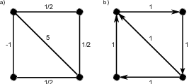
In [8] it is shown that the smallest non-trivial eigenvalue $\lambda_{1}$ of non-complete undirected graphs $\Gamma\in\mathbb{G}^{\mathrm{u}+}$ with nonnegative weights satisfies $\lambda_{1}\leq 1$ . It is tempting to conjecture that $\min_{i\neq 0}\Re(\lambda_{i})\leq 1$ for all non-complete undirected graphs with positive and negative weights and for all non-complete directed graphs with nonnegative weights. However, the two examples in Figure 2 show that this is, in general, not true. For both, the non-complete graph $\Gamma_{1}\in\mathbb{G}^{\mathrm{u}}$ in Figure 2 (a) and the non-complete graph $\Gamma_{2}\in\mathbb{G}^{+}$ in Figure 2 (b) we have $\min_{i\neq 0}\Re(\lambda_{i})>1$ . Thus, there exist non-complete graphs $\Gamma_{1}\in\mathbb{G}^{\mathrm{u}}$ and $\Gamma_{2}\in\mathbb{G}^{+}$ for which the smallest non-zero real part of the eigenvalues is larger than the smallest non-zero eigenvalue of all non-complete graphs $\Gamma\in\mathbb{G}^{\mathrm{u}+}$ . This observation has interesting consequences for the synchronization of coupled oscillators, see [1].

4. Spectrum of $\Delta$ and isolated components of $\Gamma$

We have the following simple observation:

Lemma 4.1.

Consider a graph $\Gamma\in\mathbb{G}$ and let $\Gamma_{i},1\leq i\leq r$ be its strongly connected components. Furthermore, let the Laplace operator $\Delta$ be represented in Frobenius normal form (10). Then,

$(i)$

If $\Gamma_{i}$ is isolated then $\Delta_{ij}=0$ for all $j>i$ .
$(ii)$

If $\Gamma_{i}$ is quasi-isolated then the row sums of $\Delta_{i,(i+1)}\ldots\Delta_{ir}$ add up to zero.

Moreover, if $\Gamma\in\mathbb{G}^{+}$ then

$(iii)$

$\Gamma_{i}$ is isolated if and only if $\Delta_{ij}=0$ for all $j>i$ .
$(iv)$

$\Gamma_{i}$ is quasi-isolated if and only if the row sums of $\Delta_{i,(i+1)}\ldots\Delta_{ir}$ add up to zero.

Lemma 4.2.

Every graph $\Gamma\in\mathbb{G}$ contains at least one isolated strongly connected component. Furthermore, $\Gamma\in\mathbb{G}$ contains exactly one isolated strongly connected component if and only if $\Gamma$ contains a spanning tree.

Proof.

This follows immediately from the Frobenius normal form of $\Delta$ . ∎

In particular, every undirected graph $\Gamma\in\mathbb{G}^{\mathrm{u}}$ is strongly connected and isolated.

In general, it is not true that the spectrum of an induced subgraph $\Gamma^{\prime}$ of $\Gamma$ is contained in the spectrum of the whole $\Gamma$ , i. e. $\mathrm{spec}(\Delta(\Gamma^{\prime}))\nsubseteq\mathrm{spec}(\Delta(\Gamma))$ . However, we have the following result:

Proposition 4.1.

Let $\Gamma\in\mathbb{G}$ and $\Gamma^{\prime}$ be an induced subgraph of $\Gamma$ . If one of the following conditions is satisfied

(i)

$\Gamma^{\prime}$ consists of $1\leq p\leq r$ strongly connected components of $\Gamma$ and is quasi-isolated,
(ii)

$\Gamma^{\prime}$ is isolated,

then

\mathrm{spec}(\Delta(\Gamma^{\prime}))\subseteq\mathrm{spec}(\Delta(\Gamma)).

Proof.

$(i)$ First, assume that $\Gamma^{\prime}$ is quasi-isolated and consists of $p$ strongly connected components of $\Gamma$ . Without loss of generality we assume that $\Gamma^{\prime}=\cup_{i=1}^{p}\Gamma_{i}$ . Since $\Gamma^{\prime}$ is quasi-isolated we have for all vertices $i\in V^{\prime}$ :

d^{\mathrm{in}}_{i}=\sum_{j\in V}w_{ij}=\sum_{j\in V^{\prime}}w_{ij}+\sum_{j\in V\setminus V^{\prime}}w_{ij}=\sum_{j\in V^{\prime}}w_{ij}

Thus, the in-degree of each vertex $i\in V^{\prime}$ is not affected by the vertices in $V\setminus V^{\prime}$ . Using (10) and (11) we obtain

\mathrm{spec}(\Delta(\Gamma^{\prime}))=\bigcup_{i=1}^{p}\mathrm{spec}(\Delta_{i})\subseteq\bigcup_{i=1}^{r}\mathrm{spec}(\Delta_{i})=\mathrm{spec}(\Delta(\Gamma)).

$(ii)$ Now assume that $\Gamma^{\prime}$ is isolated. Observe that each isolated induced subgraph $\Gamma^{\prime}$ of $\Gamma$ has to consist of $p$ , $1\leq p\leq r$ strongly connected components of $\Gamma$ . Thus, the second assertion follows from the first one. ∎

We will make use of the following theorem by Taussky [23].

Theorem 4.1 ([23]).

A complex $n\times n$ matrix $A$ is non-singular if $A$ is irreducible and $|A_{ii}|\geq\sum_{j\neq i}|A_{ij}|$ with equality in at most $n-1$ cases.

Lemma 4.3.

Let $\Gamma\in\mathbb{G}^{+}$ be a graph with nonnegative weights and let $\Gamma_{i}$ , $1\leq i\leq r$ be its strongly connected components. Furthermore, let $\Delta$ be represented in Frobenius normal form. Then, zero is an eigenvalue (in fact a simple eigenvalue) of $\Delta_{i}$ if and only if $\Gamma_{i}$ is isolated.

Proof.

We observe that since $\Gamma\in\mathbb{G}^{+}$ , it follows that $d_{j}^{\mathrm{in}}\neq 0$ for all $j\in\Gamma_{i}$ and hence $\Delta_{i}$ is irreducible. First assume that $\Gamma_{i}$ is not isolated. Assume further that $\Gamma_{i}$ consists of more than one vertex. Then there exists a vertex $k\in V_{i}$ s.t. $w_{kl}\neq 0$ for some $l\notin V_{i}$ . For vertex $k$ we have

|(\Delta_{i})_{kk}|=1>\frac{\sum_{j\in V_{i}}|w_{kj}|}{\sum_{j\in V}|w_{kj}|}=\sum_{j\in V_{i}}\frac{|w_{kj}|}{|d^{\mathrm{in}}_{k}|}=\sum_{j\in V_{i}}|(\Delta_{i})_{kj}|.

For all other $j\in V_{i}$ we have

|(\Delta_{i})_{jj}|=1\geq\sum_{l\in V_{i}}\frac{|w_{jl}|}{|d^{\mathrm{in}}_{j}|}=\sum_{l\in V_{i}}|(\Delta_{i})_{jl}|

and hence by Theorem 4.1, $0$ is not an eigenvalue of $\Delta_{i}$ . If $\Gamma_{i}$ consists of one vertex, then $1$ is the only eigenvalue of $\Delta_{i}$ and hence $0$ is not an eigenvalue of $\Delta_{i}$ .

Now we assume that $\Gamma_{i}$ is isolated and consists of more than one vertex. We consider the operator $P_{i}:=I_{i}-\Delta_{i}$ , where $I_{i}$ is the identity operator on $\Gamma_{i}$ . Since all row sums of $P_{i}$ are equal to one, it follows that the spectral radius $\rho$ of $P_{i}$ is equal to one. Moreover, since $\Gamma\in\mathbb{G}^{+}$ , it follows that $P_{i}$ is non-negative and irreducible. The Perron-Frobenius theorem implies that $\rho=1$ is a simple eigenvalue of $P_{i}$ and hence, by (15), $0$ is a simple eigenvalue of $\Delta_{i}$ . If $\Gamma_{i}$ is an isolated vertex, then clearly $0$ is a simple eigenvalue of $\Delta_{i}$ . ∎

Theorem 4.2.

For a graph $\Gamma\in\mathbb{G}^{+}$ the following four statements are equivalent:

$(i)$

The multiplicity $m_{1}(P)$ of the eigenvalue one of $P$ is equal to $k$ .
$(ii)$

The multiplicity $m_{0}(\Delta)$ of the eigenvalue zero of the Laplace operator $\Delta$ is equal to $k$ .
$(iii)$

There exist $k$ isolated strongly connected components in $\Gamma$ .
$(iv)$

The minimum number of directed trees needed to span the whole graph is equal to $k$ .

Proof.

$(i)\Leftrightarrow(ii)$ follows from (15). $(ii)\Leftrightarrow(iii)$ follows from Lemma 4.3 and (11). $(iii)\Leftrightarrow(iv)$ follows from the Frobenius normal form and Lemma 4.1 ( $iii$ ). ∎

A similar result was obtained for the algebraic graph Laplace operator $L=D-W$ in [24]. In the presence of negative weights, Theorem 4.2 is not true anymore. However, for general graphs $\Gamma\in\mathbb{G}$ we have the following:

Corollary 4.1.

For a graph $\Gamma\in\mathbb{G}$ we have:

$(i)$

$m_{1}(P)=m_{0}(\Delta)$ .
$(ii)$

The number of isolated strongly connected components in $\Gamma$ is equal to the minimum number of directed trees needed to span $\Gamma$ .
$(iii)$

The number of isolated strongly connected components in $\Gamma$ is less or equal to the multiplicity of the eigenvalue zero of $\Delta$ .

Proof.

The first two statements follows exactly in the same way as in Theorem 4.2, since the proof is not affected by the presence of negative weights. The third assertion follows from the observation that for every isolated strongly connected component $\Gamma_{i}$ the Laplace operator $\Delta_{i}$ has at least one eigenvalue equal to zero. This observation follows immediately from Proposition 4.1 and Proposition 3.1 $(i)$ . ∎

5. Directed acyclic graphs

Definition 5.1.

A directed cycle is a cycle with all edges being oriented in the same direction. A vertex is a cyclic vertex if it is contained in at least one directed cycle. A graph is an directed acyclic graph if none of its vertices are cyclic. The class of all directed acyclic graphs is denoted by $\mathbb{G}^{\mathrm{ac}}$ .

Note that a directed acyclic graph is not necessarily a directed tree, because we do not exclude the existence of topological cycles in the graph. If $\Delta$ is represented in the Frobenius normal form, then we immediately obtain the following:

Lemma 5.1.

The following three statements are equivalent:

(i)

$\Gamma\in\mathbb{G}^{\mathrm{ac}}$ is a directed acyclic graph.
(ii)

Every strongly connected component of $\Gamma$ consists of exactly one vertex.
(iii)

$\Delta$ represented in Frobenius normal form is upper triangular.

Theorem 5.1.

(i)

If $\Gamma\in\mathbb{G}^{\mathrm{ac}}$ is a directed acyclic graph, then $\mathrm{spec}(\Delta)\subseteq\{0,1\}$ . Furthermore, $m_{0}(\Delta)=|V\setminus V_{R}|$ and $m_{1}(\Delta)=|V_{R}|$ .
(ii)

$\Gamma\in\mathbb{G}^{+}$ and $\mathrm{spec}(\Delta)\subseteq\{0,1\}$ if and only if $\Gamma\in\mathbb{G}^{ac,+}$ .

Proof.

The first part follows immediately from Lemma 5.1, the definition of $\Delta$ , and (11). Thus, we only have to prove that if $\Gamma\in\mathbb{G}^{+}$ and $\mathrm{spec}(\Delta)\subseteq\{0,1\}$ then $\Gamma\in\mathbb{G}^{ac,+}$ . Assume the converse, i.e. assume that $\Gamma\in\mathbb{G}^{+}$ and $\mathrm{spec}(\Delta)\subseteq\{0,1\}$ but $\Gamma\notin\mathbb{G}^{ac,+}$ . Then, by Lemma 5.1 there exists a strongly connected component $\Gamma_{i}$ in $\Gamma$ consisting of at least two vertices. First, assume that $\Gamma_{i}$ is isolated. Then, by Lemma 4.3 exactly one eigenvalue of $\Delta_{i}$ is equal to zero. Using Proposition 4.1 and Corollary 3.1 we conclude that there exists an eigenvalue $\lambda\in\mathrm{spec}(\Delta)$ s.t. $\Re(\lambda)\geq\frac{n_{i}}{n_{i}-1}>1$ where $n_{i}=|V_{i}|>1$ . This is the desired contradiction. Now assume that $\Gamma_{i}$ is not isolated. By Lemma 4.3, all eigenvalues of $\Delta_{i}$ are non-zero. Since $\Gamma\in\mathbb{G}^{+}$ , $P_{i}$ is non-negative and irreducible. The Perron-Frobenius theorem implies that the spectral radius $\rho$ of $P_{i}$ is positive and is an eigenvalue of $P_{i}$ . By (15), $1-\rho$ is an eigenvalue of $\Delta_{i}$ that satisfies $1>1-\rho>0$ . Hence, we have a contradiction to the assumption that $\mathrm{spec}(\Delta)\subseteq\{0,1\}$ . ∎

Corollary 5.1.

If $k$ eigenvalues of $\Delta$ are not equal to $0$ or $1$ , then there exists at least $k$ cyclic vertices in the graph.

6. Extremal eigenvalues

In this section, we study eigenvalues $\lambda$ of $\Delta$ that satisfy $|1-\lambda|=r$ , i. e. eigenvalues that are boundary points of the disc $\mathcal{D}(1,r)$ in Proposition 3.2.

Definition 6.1.

Let $\Gamma\in\mathbb{G}$ and $\Gamma^{\prime}$ be an induced subgraph of $\Gamma$ . The induced subgraph $\Gamma^{\prime}$ is said to be maximal if all vertices $i\in V^{\prime}$ satisfy

r(i)=\max_{l}r(l)=r,

where as before

r(i):=\frac{\sum_{j\in V}|w_{ij}|}{|d^{\mathrm{in}}_{i}|}.

Note that, if we exclude isolated vertices, then every graph with nonnegative weights $\Gamma\in\mathbb{G}^{+}$ is maximal. Thus, in particular, every connected graph $\Gamma\in\mathbb{G}^{\mathrm{u}+}$ is maximal.

Proposition 6.1.

Let $\lambda\neq 0$ be an eigenvalue of $\Delta$ that satisfies $|1-\lambda|=r$ . Then $\Gamma$ possesses a maximal, isolated, strongly connected component that consists of at least two vertices.

Before we prove Proposition 6.1, we consider the following lemma.

Lemma 6.1.

Let $\lambda\neq 1$ , be an eigenvalue of $P$ that satisfies $|\lambda|=r$ . Then $\lambda$ is an eigenvalue of the Dirichlet operator $P_{k}$ that corresponds to the strongly connected component $\Gamma_{k}$ for some $k$ . Furthermore, $\Gamma_{k}$ consists of at least two vertices and the corresponding eigenfunction $u$ for $\lambda$ satisfies $|u(i)|=\mathrm{const}$ for all $i\in V_{k}$ .

Proof.

From (10) and (11) it follow that $\lambda$ is an eigenvalue of $P_{k}$ for some $1\leq k\leq z$ . Since we assume that $\lambda\neq 1$ it follows that $V_{R}\neq\emptyset$ and hence $r\geq 1$ . This in turn implies that $\Gamma_{k}$ consists of at least two vertices because otherwise by Theorem 5.1 and (15), $P_{k}$ has only one eigenvalue which is either equal to zero or one. So we only have to prove that $|u(i)|=\mathrm{const}$ for all $i\in V_{k}$ .

Assume that $|u|$ is not constant on $V_{k}$ . Since $\Gamma_{k}$ is strongly connected, there exists two vertices $i,j$ in $V_{k}$ that satisfy $w_{ij}\neq 0$ and $|u(j)|<|u(i)|=\max_{l\in V_{k}}|u(l)|$ . Again, since $\lambda\neq 1$ it follows that $i\in V_{R}$ and hence we have

	$\displaystyle\left\|P_{k}u(i)\right\|$	$\displaystyle=$	$\displaystyle\left\|\frac{1}{d^{\mathrm{in}}_{i}}\sum_{l\in V_{k}}w_{il}u(l)\right\|\leq\frac{1}{\|d^{\mathrm{in}}_{i}\|}\sum_{l\in V_{k}}\|w_{il}\|\|u(l)\|$
		$\displaystyle<$	$\displaystyle r(i)\max_{l\in V_{k}}\|u(l)\|\leq r\max_{l\in V_{k}}\|u(l)\|.$

On the other hand we have

(18)

\left|P_{k}u(i)\right|=|\lambda||u(i)|=r\max_{l\in V_{k}}|u(l)|.

This is a contradiction to the last equation. ∎

Now we prove Proposition 6.1.

Proof.

For simplicity, we consider $P$ instead of $\Delta$ . Formulated in terms of $P$ we have to show the following: Let $\lambda\neq 1$ be an eigenvalue of $P$ that satisfies $|\lambda|=r$ then $\Gamma$ possesses an isolated, maximal, strongly connected component consisting of at least two vertices. As in the proof of Lemma 6.1 one can show that $\lambda$ is an eigenvalue of the operator $P_{k}$ that corresponds to a strongly connected component $\Gamma_{k}$ consisting of at least two vertices.

First we show that all vertices in $\Gamma_{k}$ are not quasi-isolated. Assume that at least one vertex, say vertex $l$ , in $\Gamma_{k}$ is quasi-isolated. Then

P_{k}u(l)=u(l)=\lambda u(l).

Since $\lambda\neq 1$ it follows that $u(l)=0$ . Thus, we have $|u(l)|<\max_{j\in V_{k}}|u(j)|$ which is a contradiction to Lemma 6.1.

Now we prove that $\Gamma_{k}$ is isolated. Assume that $\Gamma_{k}$ is not isolated, then there exists a vertex $i\in V_{k}$ and a neighbor $j\notin V_{k}$ of $i$ . Thus, we have for the vertex $i$ that

$\displaystyle\left\|P_{k}u(i)\right\|$	$\displaystyle=$	$\displaystyle\left\|\frac{1}{d^{\mathrm{in}}_{i}}\sum_{l\in V_{k}}w_{il}u(l)\right\|\leq\frac{1}{\|d^{\mathrm{in}}_{i}\|}\sum_{l\in V_{k}}\|w_{il}\|\|u(l)\|$
	$\displaystyle<$	$\displaystyle\frac{1}{\|d^{\mathrm{in}}_{i}\|}\sum_{l\in V}\|w_{il}\|\max_{l\in V_{k}}\|u(l)\|=r(i)\max_{l\in V_{k}}\|u(l)\|$
	$\displaystyle\leq$	$\displaystyle r\max_{l\in V_{k}}\|u(l)\|.$

On the other hand, we have

(19)

\left|P_{k}u(i)\right|=|\lambda||u(i)|=r|u(i)|.

Comparing these two equations yields

|u(i)|<\max_{l\in V_{k}}|u(l)|.

Again, this is a contradiction to Lemma 6.1.

Finally, we have to prove that the strongly connected component $\Gamma_{k}$ is maximal. Assume that $\Gamma_{k}$ not maximal. Then there exists a vertex, say $i\in V_{k}$ , such that $r(i)<r$ . We conclude that

$\displaystyle\|P_{k}u(i)\|$	$\displaystyle=$	$\displaystyle\left\|\frac{1}{d^{\mathrm{in}}_{i}}\sum_{l\in V_{k}}w_{il}u(l)\right\|\leq\frac{1}{\|d^{\mathrm{in}}_{i}\|}\sum_{l\in V_{k}}\|w_{il}\|\|u(l)\|$
	$\displaystyle\leq$	$\displaystyle\frac{1}{\|d^{\mathrm{in}}_{i}\|}\sum_{l\in V}\|w_{il}\|\max_{l\in V_{k}}\|u(l)\|=r(i)\max_{l\in V_{k}}\|u(l)\|$
	$\displaystyle<$	$\displaystyle r\max_{l\in V_{k}}\|u(l)\|.$

Together with (19) this implies that $|u(i)|<\max_{l\in V_{k}}|u(l)|$ . Again, this is a contradiction to Lemma 6.1. ∎

In Proposition 6.1 we have to exclude the eigenvalue $\lambda=0$ . However, if we assume that all vertices are not quasi-isolated, Proposition 6.1 also holds for $\lambda=0$ .

Proposition 6.2.

Let $\Gamma\in\mathbb{G}$ and assume that all vertices are not quasi-isolated. If $\lambda=0$ is an eigenvalue of $\Delta$ that satisfies $|1-\lambda|=r$ , then there exists a maximal, isolated, strongly connected component consisting of at least two vertices in $\Gamma$ .

Proof.

Since $V=V_{R}$ we have for all $i\in V$ that $r(i)\geq 1$ . By assumption, we have $1=r$ and hence $r(i)=1$ for all $i\in V$ . This implies that every strongly connected component in $\Gamma$ is maximal. By Lemma 4.2 every graph contains an isolated strongly connected component. Since $\lambda=0$ and we exclude quasi-isolated vertices it follows that there exists an isolated maximal strongly connected component in $\Gamma$ that consists of at least two vertices. ∎

7. $k$ -partite graphs and anti- $k$ -partite graphs

7.1. $k$ -partite graphs

Definition 7.1.

$\Gamma\in\mathbb{G}$ is $k$ -partite, $k\geq 2$ , if $d^{\mathrm{in}}_{i}\neq 0$ for all $i\in V$ and the vertex set $V$ consists of $k$ nonempty subsets $V_{1},\ldots,V_{k}$ such that the following holds: There are only edges from vertices $j\in V_{q-1}$ to vertices $i\in V_{q}$ , $q=1,\ldots,k$ , if $\frac{w_{ij}}{d^{\mathrm{in}}_{i}}>0$ and if $k$ is even from vertices $j\in V_{q+l}$ to vertices $i\in V_{q}$ , $q=1,\ldots,k$ , if $\frac{w_{ij}}{d^{\mathrm{in}}_{i}}<0$ where $l=\frac{k}{2}-1\in{\mathbb{N}}$ and we identify $V_{k+1}$ with $V_{1}$ .

The condition $l=\frac{k}{2}-1\in{\mathbb{N}}$ implies that, in a $k$ -partite graph, there can only exists weights satisfying $\frac{w_{ij}}{d^{\mathrm{in}}_{i}}<0$ if $k$ is even. The special choice of $l$ ensures that the distance between different neighbors of one particular vertex, say vertex $i$ , is a multiple of $\frac{k}{2}$ . If the distance of two neighbors $s,t$ of $i$ is an odd multiple of $\frac{k}{2}$ , then $s,t$ belong to different subsets and $\frac{w_{is}}{w_{it}}<0$ . If the distance between $s,t$ is an even multiple of $\frac{k}{2}$ , then $s,t$ belong to the same subset and $\frac{w_{is}}{w_{it}}>0$ .

Theorem 7.1.

$\Gamma\in\mathbb{G}$ contains a $k$ -partite isolated maximal strongly connected component if and only if $1-re^{\pm 2\pi i\frac{1}{k}}$ are eigenvalues of $\Delta$ .

Proof.

Again, for technical reasons, we consider $P$ instead of $\Delta$ . Since the eigenvalues appear in complex conjugate pairs (Proposition 3.1 (ii)), it is sufficient to show that $re^{2\pi i\frac{1}{k}}$ is an eigenvalue of $P$ . Assume that $\Gamma$ contains a $k$ -partite isolated maximal strongly connected component $\Gamma_{p}$ . We claim that the function

u^{1}(j)=\left\{\begin{array}[]{c}e^{2\pi i\frac{k}{k}}\\ e^{2\pi i\frac{k-1}{k}}\\ \vdots\\ e^{2\pi i\frac{1}{k}}\end{array}\right.\begin{array}[]{c}\mbox{ if }j\in V_{p,1}\\ \mbox{ if }j\in V_{p,2}\\ \vdots\\ \mbox{ if }j\in V_{p,k},\end{array}

where $V_{p,1},\ldots,V_{p,k}$ is a $k$ -partite decomposition of $V_{p}$ , is an eigenfunction for the eigenvalue $re^{2\pi i\frac{1}{k}}$ of $P_{p}$ . For any $j\in V_{p,q}$ , $1\leq q\leq k$ , we have

$\displaystyle P_{p}u^{1}(j)$	$\displaystyle=$	$\displaystyle\frac{1}{d_{j}^{\mathrm{in}}}\sum_{t\in V_{p}}w_{jt}u^{1}(t)$
	$\displaystyle=$	$\displaystyle\frac{1}{d_{j}^{\mathrm{in}}}\left(\sum_{t\in V_{p,q-1}}w_{jt}u^{1}(t)+\sum_{t\in V_{p,q+l}}w_{jt}u^{1}(t)\right)$
	$\displaystyle=$	$\displaystyle\frac{1}{d_{j}^{\mathrm{in}}}\left(\sum_{t\in V_{p,q-1}}w_{jt}e^{2\pi i\frac{1}{k}}u^{1}(j)+\sum_{t\in V_{p,q+l}}w_{jt}e^{-\pi i}e^{2\pi i\frac{1}{k}}u^{1}(j)\right)$
	$\displaystyle=$	$\displaystyle\frac{1}{\|d^{\mathrm{in}}_{j}\|}\sum_{t\in V_{p,q-1}}\|w_{jt}\|e^{2\pi i\frac{1}{k}}u^{1}(j)-\frac{1}{\|d^{\mathrm{in}}_{j}\|}\sum_{t\in V_{p,q+l}}\|w_{jt}\|e^{-\pi i}e^{2\pi i\frac{1}{k}}u^{1}(j)$
	$\displaystyle=$	$\displaystyle\frac{1}{\|d^{\mathrm{in}}_{j}\|}\sum_{t\in V_{p}}\|w_{jt}\|e^{2\pi i\frac{1}{k}}u^{1}(j)=\frac{1}{\|d^{\mathrm{in}}_{j}\|}\sum_{t\in V}\|w_{jt}\|e^{2\pi i\frac{1}{k}}u^{1}(j)$
	$\displaystyle=$	$\displaystyle r(j)e^{2\pi i\frac{1}{k}}u^{1}(j)=re^{2\pi i\frac{1}{k}}u^{1}(j),$

where we used that the $k$ -partite component $\Gamma_{p}$ is isolated and maximal. We conclude that $re^{2\pi i\frac{1}{k}}$ is an eigenvalue of $P_{p}$ and, by Proposition 4.1, $re^{2\pi i\frac{1}{k}}$ is an eigenvalue of $P$ .

Now assume that $re^{2\pi i\frac{1}{k}}$ is an eigenvalue of $P$ . Since $|re^{2\pi i\frac{1}{k}}|=r$ and $re^{2\pi i\frac{1}{k}}\neq 1$ , Proposition 6.1 implies that $\Gamma$ contains an isolated maximal strongly connected component $\Gamma_{p}$ and $re^{2\pi i\frac{1}{k}}$ is an eigenvalue of the corresponding Dirichlet operator $P_{p}$ . We only have to prove that $\Gamma_{p}$ is $k$ -partite.

Let $u\in C(V_{p})$ be an eigenfunction for the eigenvalue $re^{2\pi i\frac{1}{k}}$ . On the one hand, since $\Gamma_{p}$ is maximal and isolated, all $j\in V_{p}$ satisfy

(20)		$\displaystyle P_{p}u(j)$	$\displaystyle=$	$\displaystyle re^{2\pi i\frac{1}{k}}u(j)=\frac{1}{\|d^{\mathrm{in}}_{j}\|}\sum_{t\in V}\|w_{jt}\|e^{2\pi i\frac{1}{k}}u(j)$
(21)			$\displaystyle=$	$\displaystyle\frac{1}{\|d^{\mathrm{in}}_{j}\|}\sum_{t\in V_{p}}\|w_{jt}\|e^{2\pi i\frac{1}{k}}u(j).$

On the other hand

(22)

P_{p}u(j)=\frac{1}{d^{\mathrm{in}}_{j}}\sum_{t\in V_{p}}w_{jt}u(t).

Comparing these two equations yields

(23)

\sum_{t\in V_{p}}\frac{|w_{jt}|}{|d^{\mathrm{in}}_{j}|}=\sum_{t\in V_{p}}\frac{w_{jt}}{d^{\mathrm{in}}_{j}}\frac{u(t)}{u(j)}e^{-2\pi i\frac{1}{k}}.

Lemma 6.1 implies that the eigenfunction $u$ satisfies $|u(t)|=|u(j)|$ for all $j,t\in V_{p}$ . Thus, $\frac{u(t)}{u(j)}e^{-2\pi i\frac{1}{k}}$ is a complex number whose absolute value is equal to one. Since we consider only real weights, we have equality in (23) if

(24)

u(j)=e^{-2\pi i\frac{1}{k}}u(t),

whenever $\frac{w_{jt}}{d^{\mathrm{in}}_{j}}>0$ and

u(j)=-e^{-2\pi i\frac{1}{k}}u(t)=e^{-\pi i}e^{-2\pi i\frac{1}{k}}u(t),

whenever $\frac{w_{jt}}{d^{\mathrm{in}}_{j}}<0$ .

First, assume that $\frac{w_{ij}}{d^{\mathrm{in}}_{i}}>0$ for all edges in $\Gamma_{p}$ . If $t$ is a neighbor of $j$ then the eigenfunction has to satisfy equation (24). Since $\Gamma_{p}$ is strongly connected we can uniquely assign to each vertex $i$ a value $u(i)$ such that every $k$ -th vertex in a directed path has the same value since $\left(e^{-2\pi i\frac{1}{k}}\right)^{k}=1$ . Now decompose the vertex set into $k$ non-empty subsets s.t. all vertices with the same $u$ -value belong to the same subset of $V_{p}$ . This yields a $k$ -partite decomposition of $\Gamma_{p}$ .

If there also exist edges s.t. $\frac{w_{ij}}{d^{\mathrm{in}}_{i}}<0$ is satisfied, then the crucial observation is that if $\frac{w_{jt}}{d^{\mathrm{in}}_{j}}<0$ for some $j$ and $t$ then there has to exist another neighbor $s$ of $j$ s.t. $\frac{w_{js}}{d^{\mathrm{in}}_{j}}>0$ . We conclude that every vertex $j$ has at least one neighbor $s$ such that $\frac{w_{js}}{d_{j}^{\mathrm{in}}}>0$ . Thus, there exist $k$ different $u$ -values and we can find a $k$ -partite decomposition of $V_{p}$ similarly as in the case studied before. ∎

Even if we do not require that the $k$ -partite component is maximal we have:

Corollary 7.1.

Let $\Gamma\in\mathbb{G}$ contain a $k$ -partite isolated strongly connected component $\Gamma_{p}$ , and let $r(j)=c$ for all $j\in V_{p}$ and some constant $c$ . Then $1-ce^{\pm 2\pi i\frac{1}{k}}$ are eigenvalues of $\Delta$ .

Theorem 7.1 can be used to characterize the graph $\Gamma\in\mathbb{G}^{+}$ whose spectrum contains the distinguished eigenvalues $1-e^{\pm 2\pi i\frac{1}{n}}$ in Figure 1. As a special case of Theorem 7.1 we obtain:

Corollary 7.2.

Let $\Gamma\in\mathbb{G}^{+}$ be a graph with $n$ vertices. Then, $1-e^{\pm 2\pi i\frac{1}{n}}$ is an eigenvalue of $\Delta(\Gamma)$ iff $\Gamma$ is a directed cycle.

Definition 7.2.

The associated positive graph $\Gamma^{+}\in\mathbb{G}^{+}$ of a graph $\Gamma\in\mathbb{G}$ is obtained from $\Gamma$ by replacing every weight $w_{ij}$ by its absolute value $|w_{ij}|$ . The eigenvalues of $\Gamma^{+}$ are denoted by $\lambda^{+}_{0},\ldots\lambda_{n-1}^{+}$ and the Laplace operator defined on the graph $\Gamma^{+}$ is denoted by $\Delta^{+}$ .

Clearly, a graph $\Gamma\in\mathbb{G}^{+}$ with nonnegative weights coincides with its associated positive graph, i. e. $\Gamma=\Gamma^{+}$ .

Remark.

It is also possible to define the associated negative graph $\Gamma^{-}$ of a graph $\Gamma$ that is obtained from $\Gamma$ by replacing every weight $w_{ij}$ by $-|w_{ij}|$ . Note however, that by Proposition 3.1 $(v)$ the graphs $\Gamma^{-}$ and $\Gamma^{+}$ are isospectral. Thus, we will only consider $\Gamma^{+}$ in the following.

Theorem 7.2.

Let $\Gamma\in\mathbb{G}$ be a $k$ -partite graph and $r(j)=r$ for all $j\in V$ . Then, the spectra of $\Delta^{+}$ and $\Delta$ satisfy the following relation: $\lambda^{+}\in\mathrm{spec}(\Delta^{+})$ iff $1-re^{\pm 2\pi i\frac{1}{k}}(1-\lambda^{+})\in\mathrm{spec}(\Delta)$ .

Proof.

Let the function $u$ satisfy $\Delta^{+}u=\lambda^{+}u$ . We define a new function $v$ in the following way:

(25)

v(j)=\left\{\begin{array}[]{r c l}e^{2\pi i\frac{1}{k}}u(j)&\quad if&j\in V_{1}\\ e^{2\pi i\frac{2}{k}}u(j)&\quad if&j\in V_{2}\\ \vdots&&\\ e^{2\pi i\frac{k}{k}}u(j)&\quad if&j\in V_{k},\end{array}\right.

where $V_{1},\ldots,V_{k}$ is a $k$ -partite decomposition of $V$ . We show that $v$ is an eigenfunction for $\Delta$ and the corresponding eigenvalue is given by $(1-re^{-2\pi i\frac{1}{k}}(1-\lambda^{+}))$ . For any $j\in V_{q}$ and $1\leq q\leq k$ , we have

$\displaystyle\Delta v(j)$	$\displaystyle=$	$\displaystyle v(j)-\frac{1}{d_{j}^{\mathrm{in}}}\sum_{t\in V_{q-1}}w_{jt}v(t)-\frac{1}{d_{j}^{\mathrm{in}}}\sum_{t\in V_{q+l}}w_{jt}v(t)$
	$\displaystyle=$	$\displaystyle e^{2\pi i\frac{q}{k}}u(j)-\frac{1}{\|d_{j}^{\mathrm{in}}\|}\sum_{t\in V_{q-1}}\|w_{jt}\|e^{2\pi i\frac{q-1}{k}}u(t)+\frac{1}{\|d_{j}^{\mathrm{in}}\|}\sum_{t\in V_{q+l}}\|w_{jt}\|e^{\pi i}e^{2\pi i\frac{q-1}{k}}u(t)$
	$\displaystyle=$	$\displaystyle e^{2\pi i\frac{q}{k}}u(j)-\frac{1}{\|d^{\mathrm{in}}_{j}\|}\sum_{t\in V}\|w_{jt}\|e^{2\pi i\frac{q-1}{k}}u(t)$
	$\displaystyle=$	$\displaystyle e^{2\pi i\frac{q}{k}}u(j)-re^{2\pi i\frac{q-1}{k}}u(j)+re^{2\pi i\frac{q-1}{k}}\underbrace{\left(u(j)-\frac{1}{\sum_{t\in V}\|w_{jt}\|}\sum_{t\in V}\|w_{jt}\|u(t)\right)}_{=\Delta^{+}u(j)=\lambda^{+}u(j)}$
	$\displaystyle=$	$\displaystyle(1-re^{-2\pi i\frac{1}{k}}(1-\lambda^{+}))v(j).$

Since the edge weights are real, $\Delta$ can be represented as a real matrix and hence $\overline{v}$ is an eigenfunction for the eigenvalue $1-re^{2\pi i\frac{1}{k}}(1-\lambda^{+}))$ .

The other direction follows in a similar way. To be more precise, for an eigenfunction $v$ of $\Delta$ we define the function $u$ by

(26)

u(j)=\left\{\begin{array}[]{r c l}e^{2\pi i\frac{1}{k}}v(j)&\quad if&j\in V_{1}\\ e^{2\pi i\frac{2}{k}}v(j)&\quad if&j\in V_{2}\\ \vdots&&\\ e^{2\pi i\frac{k}{k}}v(j)&\quad if&j\in V_{k}.\end{array}\right.

As above, one can show that $u$ is an eigenfunction for $\Delta^{+}$ and corresponding eigenvalue $1-\frac{1}{r}e^{-2\pi i\frac{1}{k}}(1-\lambda)$ . ∎

Note that in Theorem 7.2 we do not assume that $\Gamma$ is strongly connected. However, if we assume in addition that $\Gamma$ is strongly connected, then we have the following result:

Corollary 7.3.

Let $\Gamma\in\mathbb{G}$ be a strongly connected graph, and $r(j)=r$ for all $j\in V$ . Then, $\Gamma$ is $k$ -partite if and only if the spectra of $\Delta^{+}$ and $\Delta$ satisfy the following: $\lambda^{+}$ is an eigenvalue of $\Delta^{+}$ iff $1-re^{\pm 2\pi i\frac{1}{k}}(1-\lambda^{+})$ is an eigenvalue of $\Delta$ .

Proof.

One direction follows from Theorem 7.2. The other direction follows from the observation that zero is an eigenvalue of $\Delta^{+}$ and thus $1-re^{\pm 2\pi i\frac{1}{k}}$ is an eigenvalue of $\Delta$ . Since $\Gamma$ is strongly connected, it follows from Theorem 7.1 that the whole graph is $k$ -partite. ∎

Moreover, a $k$ -partite graph has the following eigenvalues:

Proposition 7.1.

Let $\Gamma\in\mathbb{G}$ be a $k$ -partite graph and $r(l)=r$ for all $l\in V$ . Then, $1-re^{2\pi i\frac{m}{k}}\in\mathrm{spec}(\Delta)$ for $1\leq m\leq k-1$ and $m$ odd. If, in addition, $\frac{w_{jt}}{d^{\mathrm{in}}_{j}}>0$ for all $j,t\in V$ , then $1-e^{2\pi i\frac{m}{k}}\in\mathrm{spec}(\Delta)$ for all $0\leq m\leq k-1$ .

Proof.

In order to prove that $1-re^{2\pi i\frac{m}{k}}$ is an eigenvalue of $\Delta$ , it is sufficient to show that $re^{2\pi i\frac{m}{k}}$ is an eigenvalue of $P$ . Consider the functions

(27)

u^{m}(j)=\left\{\begin{array}[]{r c l}e^{2\pi i\frac{mk}{k}}&\quad if&j\in V_{1}\\ e^{2\pi i\frac{m(k-1)}{k}}&\quad if&j\in V_{2}\\ \vdots&&\\ e^{2\pi i\frac{m1}{k}}&\quad if&j\in V_{k},\end{array}\right.

for $m=0,1,\ldots k-1$ . One easily checks that these functions are linearly independent if $k>2$ .

For all $j\in V_{q}$ , $q=1,\ldots,k$ , and $0\leq m\leq k-1$ we have

(28)	$\displaystyle Pu^{m}(j)$	$\displaystyle=$	$\displaystyle\frac{1}{d_{j}^{\mathrm{in}}}\sum_{t\in V_{q-1}}w_{jt}u^{m}(t)+\frac{1}{d_{j}^{\mathrm{in}}}\sum_{t\in V_{q+l}}w_{jt}u^{m}(t)$
		$\displaystyle=$	$\displaystyle\frac{1}{\|d^{\mathrm{in}}_{j}\|}\sum_{t\in V_{q-1}}\|w_{jt}\|e^{2\pi i\frac{m}{k}}u^{m}(j)-\frac{1}{\|d^{\mathrm{in}}_{j}\|}\sum_{t\in V_{q+l}}\|w_{jt}\|e^{-2\pi i\frac{ml}{k}}u^{m}(j)$
		$\displaystyle=$	$\displaystyle\frac{1}{\|d^{\mathrm{in}}_{j}\|}\sum_{t\in V_{q-1}}\|w_{jt}\|e^{2\pi i\frac{m}{k}}u^{m}(j)-\frac{1}{\|d^{\mathrm{in}}_{j}\|}\sum_{t\in V_{q+l}}\|w_{jt}\|e^{2\pi i\frac{m}{k}}e^{-\pi im}u^{m}(j).$

If $m$ is odd, then $e^{-\pi im}=-1$ and thus

$\displaystyle Pu^{m}(j)$	$\displaystyle=$	$\displaystyle\frac{1}{\|d^{\mathrm{in}}_{j}\|}\sum_{t\in V_{q-1}\cup V_{q+l}}\|w_{jt}\|e^{2\pi i\frac{m}{k}}u^{m}(j)$
	$\displaystyle=$	$\displaystyle\frac{1}{\|d^{\mathrm{in}}_{j}\|}\sum_{t\in V}\|w_{jt}\|e^{2\pi i\frac{m}{k}}u^{m}(j)$
	$\displaystyle=$	$\displaystyle re^{2\pi i\frac{m}{k}}u^{m}(j).$

Hence, $1-re^{2\pi i\frac{m}{k}}$ for $1\leq m\leq k-1$ and $m$ odd is an eigenvalue of $\Delta$ .

If in addition $\frac{w_{jt}}{d^{\mathrm{in}}_{j}}>0$ for all $j$ and $t$ in $V$ , then $r=1$ and there are only edges from vertices in $V_{q-1}$ to vertices in $V_{q}$ . Thus, the second term on the r.h.s. of (28) vanishes and we can conclude that

	$\displaystyle Pu^{m}(j)$	$\displaystyle=$	$\displaystyle\frac{1}{\|d^{\mathrm{in}}_{j}\|}\sum_{t\in V_{q-1}}\|w_{jt}\|e^{2\pi i\frac{m}{k}}u^{m}(j)=\frac{1}{\|d^{\mathrm{in}}_{j}\|}\sum_{t\in V}\|w_{jt}\|e^{2\pi i\frac{m}{k}}u^{m}(j)$
		$\displaystyle=$	$\displaystyle re^{2\pi i\frac{m}{k}}u^{m}(j)=e^{2\pi i\frac{m}{k}}u^{m}(j).$

This shows that $1-e^{2\pi i\frac{m}{k}}$ for all $m=0,\ldots,k-1$ is an eigenvalue of $\Delta$ . ∎

7.2. Anti- $k$ -partite graphs

In this section, we study graphs that are closely related to $k$ -partite graphs. We call those graphs anti- $k$ -partite graphs since they have the same topological structure as $k$ -partite graphs but compared to $k$ -partite graphs, the normalized weights $\frac{w_{ij}}{d^{\mathrm{in}}_{i}}$ in anti- $k$ -partite graphs have always the opposite sign.

Definition 7.3.

$\Gamma\in\mathbb{G}$ is anti- $k$ -partite, for $k\geq 2$ and $k$ even, if $d^{\mathrm{in}}_{i}\neq 0$ for all $i\in V$ and the vertex set $V$ consists of $k$ nonempty subsets $V_{1},\ldots,V_{k}$ such that the following holds: There are only edges from vertices $j\in V_{q-1}$ to vertices $i\in V_{q}$ if $\frac{w_{ij}}{d^{\mathrm{in}}_{i}}<0$ or from vertices $j\in V_{q+l}$ to vertices $i\in V_{q}$ if $\frac{w_{ij}}{d^{\mathrm{in}}_{i}}>0$ where $l=\frac{k}{2}-1\in{\mathbb{N}}$ and we identify $V_{k+1}$ with $V_{1}$ .

In contrast to $k$ -partite graphs, anti- $k$ -partite graphs can only be defined if $k$ is even. This follows from the observation that every vertex $i$ has at least one neighbor $j$ such that $\frac{w_{ij}}{d^{\mathrm{in}}_{i}}>0$ . Hence, every vertex $i\in V_{q}$ has at least one neighbor in $V_{q+l}$ for $q=1,\ldots,k$ . Since we require that $l=\frac{k}{2}-1\in{\mathbb{N}}$ , it follows that $k$ has to be even.

We mention the following simple observation without proof:

Proposition 7.2.

Let $\Gamma\in\mathbb{G}^{+}$ be an anti- $k$ -partite graph and $k=2+4^{m}$ , where $m=0,1,\ldots$ . Then, $\Gamma$ is disconnected and if $m\geq 1$ $\Gamma$ consists of two $\frac{k}{2}$ -partite connected components.

Theorem 7.3.

Let $\Gamma\in\mathbb{G}$ contain an anti- $k$ -partite maximal, isolated, strongly connected component, then $1+re^{\pm 2\pi i\frac{1}{k}}\in\mathrm{spec}(\Delta)$ . Furthermore, if $1+re^{\pm 2\pi i\frac{1}{k}}\in\mathrm{spec}(\Delta)$ and one of the following two conditions is satisfied

(i)

$k=4^{m}$ for $m=1,2,\ldots$
(ii)

$k=2+4^{m}$ for $m=0,1,\ldots$ and $r>1$ ,

then $\Gamma$ contains an anti- $k$ -partite isolated maximal strongly connected component.

Proof.

Assume that $\Gamma$ contains an anti- $k$ -partite maximal, isolated, strongly connected component. In exactly the same way as in Theorem 7.1 one can show that $1+re^{\pm 2\pi i\frac{1}{k}}$ is an eigenvalue of $\Delta$ . We will omit the details here. Now let $1+re^{\pm 2\pi i\frac{1}{k}}$ be an eigenvalue of $\Delta$ . Note that $1+re^{\pm 2\pi i\frac{1}{k}}\neq 0$ and thus, by Proposition 6.1, $\Gamma$ contains an maximal, isolated, strongly connected component $\Gamma_{p}$ . Furthermore, we have that $1+re^{\pm 2\pi i\frac{1}{k}}$ is an eigenvalue of $\Delta_{p}$ . By a reasoning similar to the one in the proof of Theorem 7.1 it follows that the corresponding eigenfunction for $\Delta_{p}$ satisfies

(29)

u(j)=-e^{2\pi i\frac{1}{k}}u(t)

whenever $\frac{w_{jt}}{d^{\mathrm{in}}_{j}}>0$ and

(30)

u(j)=e^{2\pi i\frac{1}{k}}u(t)

whenever $\frac{w_{jt}}{d^{\mathrm{in}}_{j}}<0$ . Now assume that $k=4^{m}$ and $\frac{w_{tj}}{d^{\mathrm{in}}_{t}}>0$ for all $t,j\in V_{p}$ .

Since $\Gamma_{p}$ is strongly connected, $k=4^{m}$ , and neighbors have to satisfy equation (29), we can uniquely assign to every vertex an $u$ -value such that every $k$ -th vertex in a directed path has the same $u$ -value. Now decompose the vertex set into $k$ non-empty subsets such that all vertices with the same $u$ -value belong to the same subset. This yields an anti- $k$ -partite decomposition of $\Gamma_{p}$ .

If there also exists edges s.t. $\frac{w_{jt}}{d^{\mathrm{in}}_{j}}<0$ is satisfied then, again, the crucial observation is that if $\frac{w_{jt}}{d^{\mathrm{in}}_{j}}<0$ for some $j$ and $t$ then there also has to exist another neighbor $s$ of $j$ s.t. $\frac{w_{js}}{d^{\mathrm{in}}_{j}}>0$ . Thus, there exist $k$ different $u$ -values. Similar to above, we can find an anti- $k$ -partite decomposition of $V_{p}$ .

If $k=2+4^{m}$ , $m=0,1,\ldots,$ the situation is different. If $\frac{w_{jt}}{d^{\mathrm{in}}_{j}}>0$ for all $j$ and $t$ , then $r=1$ . In this case, we cannot conclude that there exists an anti- $k$ -partite component since already every $\frac{k}{2}$ -th vertex in a directed path has the same $u$ -value, i.e. $(-1)^{\frac{k}{2}}(e^{2\pi i\frac{1}{k}})^{\frac{k}{2}}=1$ for $k=2+4^{m}$ , $m=0,1,\ldots$ . Thus, we crucially need that $r>1$ . In this case, every vertex $i$ has at least one neighbor $j$ such that $\frac{w_{ij}}{d^{\mathrm{in}}_{i}}<0$ . By (30) it follows that there has to exist $k$ different $u$ -values. Thus, we can obtain an anti- $k$ -partite component of $\Gamma_{p}$ in the same way as before. ∎

A simple example that shows that the assumption $r>1$ is necessary if $k=2+4^{m}$ in the last theorem. If $1-r=0$ is an eigenvalue of $\Gamma$ , then this does not imply that there exists a $2$ -partite isolated maximal strongly connected component in $\Gamma$ .

The next theorem shows that there also exists a relationship between the spectrum of an anti- $k$ -partite graph and its associated positive graph.

Theorem 7.4.

Let $\Gamma\in\mathbb{G}$ be an anti- $k$ -partite graph and $r(l)=r$ for all $l\in V$ . Then, $\lambda^{+}\in\mathrm{spec}(\Delta^{+})$ iff $1+re^{\pm 2\pi i\frac{1}{k}}(1-\lambda^{+})\in\mathrm{spec}(\Delta)$ .

We omit the proof of this theorem because it is the same as the proof of Theorem 7.2.

The next proposition is the corresponding result to Proposition 7.1 in the case of anti- $k$ -partite graphs.

Proposition 7.3.

Let $\Gamma\in\mathbb{G}$ be an anti- $k$ -partite graph, s.t. $r(l)=r$ for all $l\in V$ , then $1+re^{2\pi i\frac{m}{k}}\in\mathrm{spec}(\Delta)$ for $0\leq m\leq k-1$ , if $m$ is odd. If in addition $\frac{w_{ij}}{{d_{i}^{\mathrm{in}}}}>0$ for all $i,j\in V$ then $1-e^{2\pi i\frac{m}{k}}\in\mathrm{spec}(\Delta)$ for $0\leq m\leq k-1$ , $m$ even and $1+e^{2\pi i\frac{m}{k}}\in\mathrm{spec}(\Delta)$ for $0\leq m\leq k-1$ , $m$ odd.

Proposition 7.4.

Let $\Gamma\in\mathbb{G}$ be a strongly connected graph and $r(l)=r$ for all $l\in V$ . Assume that $k=4^{m}$ , $m=1,2,\ldots$ . Then, $\Gamma$ is $k$ -partite iff $\Gamma$ is anti- $k$ -partite.

Proof.

Assume that $\Gamma$ is $k$ -partite. By Proposition 7.1, $1-re^{2\pi i\frac{l}{k}}\in\mathrm{spec}(\Delta)$ for $0\leq l\leq k-1$ and $l$ odd. Since $k$ is of the form $k=4^{m}$ , $\frac{k}{2}+1$ is odd, and so we have $1-re^{2\pi i\frac{\frac{k}{2}+1}{k}}=1+re^{2\pi i\frac{1}{k}}\in\mathrm{spec}(\Delta)$ . From Theorem 7.3, it follows that $\Gamma$ is anti- $k$ -partite. The other direction follows in the same way by using Proposition 7.3 and Theorem 7.1. ∎

This proposition shows that if $k=4^{m}$ , $m=1,2,\ldots$ then a $k$ -partite decomposition can be obtained from an anti- $k$ -partite one, and vice versa, by relabelling the vertex sets $V_{k}$ .

7.3. Special cases: Bipartite and anti-bipartite graphs

7.3.1. Bipartite graphs

As a special case of $k$ -partite graphs we obtain:

Definition 7.4.

A graph $\Gamma\in\mathbb{G}$ is bipartite (or $2$ -partite), if $d^{\mathrm{in}}_{i}\neq 0$ for all $i\in V$ and the vertex set $V$ can be decomposed into two nonempty subsets $V_{1},V_{2}$ such that for neighbors $i$ and $j$ $\frac{w_{ij}}{d^{\mathrm{in}}_{i}}>0$ if $i$ and $j$ belong to different subsets and $\frac{w_{ij}}{d^{\mathrm{in}}_{i}}<0$ if $i$ and $j$ belong to the same subset.

In the case of undirected graphs with nonnegative weights, Definition 7.4 reduces to the usual definition of a bipartite graph.

Corollary 7.4.

A graph $\Gamma\in\mathbb{G}$ contains a maximal, isolated, bipartite strongly connected component if and only if $1+r$ is an eigenvalue of $\Delta$ .

Using Corollary 3.1 we can reformulate this as follows:

Corollary 7.5.

The spectrum of $\Delta$ contains the largest possible real eigenvalue if and only if the graph $\Gamma\in\mathbb{G}$ contains a maximal, isolated, bipartite strongly connected component.

For undirected graphs with nonnegative weights, Corollary 7.4 reduces to the well-known result that $\Gamma$ is bipartite if and only if $2$ is an eigenvalue of $\Delta$ .

Corollary 7.6.

Let $\Gamma\in\mathbb{G}$ be a bipartite graph and $r(l)=r$ for all $l\in V$ . Then, $\lambda^{+}\in\mathrm{spec}(\Delta^{+})$ iff $1+r(1-\lambda^{+})\in\mathrm{spec}(\Delta)$ .

In particular, if $\Gamma\in\mathbb{G}^{+}$ is strongly connected, then $\Gamma$ is bipartite if and only if with $\lambda$ also $2-\lambda$ is an eigenvalue of $\Delta$ , i. e. the real parts of the eigenvalues are symmetric about one.

7.3.2. Anti-bipartite graphs

As a special case of anti- $k$ -partite graphs we obtain:

Definition 7.5.

A graph $\Gamma\in\mathbb{G}$ is anti-bipartite, if $d^{\mathrm{in}}_{i}\neq 0$ for all $i\in V$ and the vertex set $V$ can be decomposed into two nonempty subsets such that for neighbors $i$ and $j$ , $\frac{w_{ij}}{d^{\mathrm{in}}_{i}}<0$ if $i$ and $j$ belong to different subsets and $\frac{w_{ij}}{d^{\mathrm{in}}_{i}}>0$ if $i$ and $j$ belong to the same subset.

Lemma 7.1.

$\Gamma\in\mathbb{G}^{+}$ is anti-bipartite if and only if the graph $\Gamma$ is disconnected and $d^{\mathrm{in}}_{i}\neq 0$ for all $i$ .

Proof.

One direction follows from Proposition 7.2.

Now assume that the graph $\Gamma\in\mathbb{G}^{+}$ is disconnected and $d^{\mathrm{in}}_{i}\neq 0$ for all $i$ . Then there exists at least two connected components such that $\frac{w_{ij}}{d^{\mathrm{in}}_{i}}>0$ for all neighbors $i$ and $j$ . Distribute the connected components (there exist maybe more than two) into two nonempty subsets $V_{1}$ and $V_{2}$ . This is an anti-bipartite decomposition of the graph. ∎

Corollary 7.7.

Let $r>1$ , then $1-r$ is an eigenvalue of $\Delta$ if and only if the graph contains an anti-bipartite maximal isolated strongly connected component.

Using Corollary 3.1 we can reformulate this as follows:

Corollary 7.8.

Assume that $r>1$ is satisfied. The spectrum of $\Delta$ contains the smallest possible real eigenvalue if and only if the graph $\Gamma\in\mathbb{G}$ contains a maximal, isolated, anti-bipartite strongly connected component.

Example 2.

Consider the graph in Figure 3. It is easy to calculate the spectrum of this graph by using the results derived in this section. First, note that the graph in Figure 3 is bipartite and anti-bipartite. Since $r(i)=3$ for all $i$ , we have $1\pm 3\in\mathrm{spec}(\Delta)$ . Zero is always an eigenvalue of $\Delta$ . The last eigenvalue is equal to $2$ since $\sum_{i}\lambda_{i}=|V_{R}|=4$ . So we have determined all eigenvalues of the graph in Figure 3.

8. Bounds for the real and imaginary parts of the eigenvalues

In this section, we will derive several bounds for the real and imaginary parts of the eigenvalues of a directed graph. In the following, we also allow loops in the graph. This slight generalization is particularly important in the next section where we introduce the neighborhood graph technique. It is straightforward to generalize the Laplace operator $\Delta$ to graphs with loops. The normalized graph Laplace operator for directed graphs with loops is defined as:

\Delta:C(V)\rightarrow C(V),

\displaystyle\Delta v(i)=\left\{\begin{array}[]{c l}v(i)-\frac{1}{d^{\mathrm{in}}_{i}}\sum_{j}w_{ij}v(j)&\mbox{if }d^{\mathrm{in}}_{i}\neq 0\\ 0&\mbox{else.}\end{array}\right.

The only difference to graphs without loops is that now $w_{ii}$ is not always equal to zero. As for graphs without loops we define $P=I-\Delta$ . Furthermore, we say that vertex $i$ is in-isolated or simply isolated if $w_{ij}=0$ for all $j\in V$ . Similarly, vertex $i$ is said to be in-quasi-isolated or simply quasi-isolated if $d_{i}^{\mathrm{in}}=0$ . In particular, an isolated vertex cannot have a loop. As before, $V_{R}:=\{i\in V:d_{i}^{\mathrm{in}}\neq 0\}$ is the set of all vertices that are not quasi-isolated.

8.1. Comparison theorems

In this section, we show that the real parts of the eigenvalues of a directed graph can be controlled by the eigenvalues of certain undirected graphs. Together with well-known estimates for undirected graphs these comparison results yield estimates the realparts of the eigenvalues of a directed graph.

We need the following definition:

Definition 8.1.

Let $\Gamma\in\mathbb{G}$ be given. The underlying graph $U(\Gamma)\in\mathbb{G}^{\mathrm{u}}$ of $\Gamma$ is obtained from $\Gamma$ by replacing each directed edge by an undirected edge of the same weight. In $U(\Gamma)$ we identify multiple edges between two vertices with one single edge. The weight of this single edge is equal to the sum of the weights of the multiple edges. Furthermore, every loop in $\Gamma$ is replace by a loop of twice the weight in $U(\Gamma)$ .

Note that the correspondence between directed graphs and their underlying graphs is not one to one. Indeed, many directed graphs can have the same underlying graph.

We recall the well-known concept of majorization:

Definition 8.2.

Let $a\in\mathbb{R}^{n}$ and $b\in\mathbb{R}^{n}$ be given. If the entries of $a$ and $b$ are arranged in increasing^‡^‡ ‡ The definition of majorization is not unique in the literature. Here, we follow the convention in [18]. In other books, see e.g. [21], majorization is defined for vectors arranged in decreasing order. Reversing the order of the elements has the following consequence: If $a$ and $b$ are two real vectors whose entries are arranged in increasing order, and $A$ and $B$ denote the vectors with the same entries arranged in decreasing order, then $a\prec b$ if and only if $B\prec A$ . order, then $b$ majorizes $a$ , in symbols $a\prec b$ , if

(34)

\sum_{i=1}^{k}a_{i}\leq\sum_{i=1}^{k}b_{i}\;\;\;\;\;\;\qquad k=1,...,n-1

and

(35)

\sum_{i=1}^{n}a_{i}=\sum_{i=1}^{n}b_{i}.

We will need the following two results:

Lemma 8.1.

[R. Rado, see e.g. [17] p.63 or [21]] If $x\prec y$ on $\mathbb{R}^{n}$ and $a\prec b$ on $\mathbb{R}^{m}$ then $(x,a)\prec(y,b)$ on $\mathbb{R}^{n+m}$ , where $(x,a)$ is the vector composed of the components of $x$ and $a$ arranged in increasing order, and similarly for $(y,b)$ .

In particular, Lemma 8.1 shows that the majorization property is preserved if we append the same entries to both $x$ and $y$ (choose $a=b$ in Lemma 8.1).

In the sequel, let the symmetric part of a matrix $M$ be denoted by $S(M):=\frac{1}{2}(M+M^{\top})$ . We make use of a classical result by Ky Fan [15]:

Lemma 8.2.

Let $\lambda(S(M))$ and $\Re[\lambda(M)]$ denote the column vectors whose components are the eigenvalues of $S(M)$ and the real parts of the eigenvalues of $M$ , respectively. If the components of $\lambda(S(M))$ and $\Re[\lambda(M)]$ are arranged in increasing order, then for every matrix $M$ we have

\lambda(S(M))\prec\Re[\lambda(M)].

Using Definition 8.1 and Definition 8.2 we state the following comparison result.

Theorem 8.1.

If $\Gamma\in\mathbb{G}$ is balanced, then

\lambda(\Delta(U(\Gamma)))\prec\Re[\lambda(\Delta(\Gamma))],

i. e. the eigenvalues of the underlying graph $U(\Gamma)$ are majorized by the real parts of the eigenvalues of $\Gamma$ .

Proof.

Recall the definition of the reduced Laplace operator $\Delta_{R}=I_{R}-D^{-1}_{R}W_{R}$ in Eq. (8). It is straightforward to generalize $\Delta_{R}$ for graphs with loops. Here however, instead of $\Delta_{R}$ we consider the reduced normalized Laplace operator $\mathcal{L}_{R}:=I_{R}-D_{R}^{-1/2}W_{R}D_{R}^{-1/2}$ . In the sequel, we will study matrix representations of $\Delta_{R}$ and $\mathcal{L}_{R}$ that will also be denoted by $\Delta_{R}$ and $\mathcal{L}_{R}$ . Since $D_{R}^{1/2}$ is nonsingular and

\Delta_{R}=D_{R}^{-1/2}\mathcal{L}_{R}D_{R}^{1/2},

it follows that $\mathcal{L}_{R}$ and $\Delta_{R}$ are similar and hence have the same spectrum. We claim that the reduced Laplace operator $\mathcal{L}_{R}$ satisfies

S(\mathcal{L}_{R}(\Gamma))=\mathcal{L}_{R}(U(\Gamma)).

Since $\Gamma$ is balanced, the degrees of the vertices satisfy

(36)

2d_{i}^{\mathrm{in}}(\Gamma)=d_{i}(U(\Gamma)).

Thus, in particular, the number of quasi-isolated vertices in $U(\Gamma)$ and $\Gamma$ is the same and so the matrices $S(\mathcal{L}_{R}(\Gamma))$ and $\mathcal{L}_{R}(U(\Gamma))$ have the same dimension.

By definition, the diagonal elements satisfy

\displaystyle S(\mathcal{L}_{R}(\Gamma))_{ii}=1-\frac{w_{ii}}{\sqrt{d_{i}^{\mathrm{in}}(\Gamma)d_{i}^{\mathrm{in}}(\Gamma)}}

and

\mathcal{L}_{R}(U(\Gamma))_{ii}=1-\frac{2w_{ii}}{\sqrt{d_{i}(U(\Gamma))d_{i}(U(\Gamma))}}=1-\frac{2w_{ii}}{\sqrt{2d_{i}^{\mathrm{in}}(\Gamma)2d_{i}^{\mathrm{in}}(\Gamma)}}=1-\frac{w_{ii}}{\sqrt{d_{i}^{\mathrm{in}}(\Gamma)d_{i}^{\mathrm{in}}(\Gamma)}}

by (36). For the off-diagonal elements, we have

\displaystyle S(\mathcal{L}_{R}(\Gamma))_{ij}=-1/2\left(\frac{w_{ij}}{\sqrt{d_{i}^{\mathrm{in}}(\Gamma)d_{j}^{\mathrm{in}}(\Gamma)}}+\frac{w_{ji}}{\sqrt{d_{j}^{\mathrm{in}}(\Gamma)d_{i}^{\mathrm{in}}(\Gamma)}}\right)

and

	$\displaystyle\mathcal{L}_{R}(U(\Gamma))_{ij}$	$\displaystyle=$	$\displaystyle-\frac{w_{ij}+w_{ji}}{\sqrt{d_{i}(U(\Gamma))d_{j}(U(\Gamma))}}$
		$\displaystyle=$	$\displaystyle-1/2\frac{w_{ij}+w_{ji}}{\sqrt{d_{i}^{\mathrm{in}}(\Gamma)d_{j}^{\mathrm{in}}(\Gamma)}},$

where we used (36). This proves our claim. Now it follows that

\lambda(\Delta_{R}(U(\Gamma)))=\lambda(\mathcal{L}_{R}(U(\Gamma)))=\lambda(S(\mathcal{L}_{R}(\Gamma)))\prec\Re(\lambda(\mathcal{L}_{R}(\Gamma)))=\Re(\lambda(\Delta_{R}(\Gamma))),

where we used Lemma 8.2 and the fact that $\mathcal{L}_{R}$ and $\Delta_{R}$ have the same spectrum. By (9), the spectrum of $\Delta(\Gamma)$ ( $\Delta(U(\Gamma))$ ) consists of all eigenvalues of $\Delta_{R}(\Gamma)$ ( $\Delta_{R}(U(\Gamma))$ ) and $|V\setminus V_{R}|$ times the eigenvalue zero. From (36) it follows that the number of quasi-isolated vertices is the same in $U(\Gamma)$ and $\Gamma$ . Hence Lemma 8.1 implies

\lambda(\Delta(U(\Gamma)))\prec\Re[\lambda(\Delta(\Gamma))].

∎

Theorem 8.1 is used in [1] to compare the synchronizability of directed and undirected networks of coupled phase oscillators.

In particular Theorem 8.1 implies:

Corollary 8.1.

For a balanced graph $\Gamma\in\mathbb{G}$ we have

\min_{i\neq 0}\lambda_{i}(\Delta(U(\Gamma)))\leq\min_{i\neq 0}\Re(\lambda_{i}(\Delta(\Gamma)))

and

\max_{i}\Re(\lambda_{i}(\Delta(\Gamma)))\leq\max_{i}\lambda_{i}(\Delta(U(\Gamma))),

where $\lambda_{0}=0$ is the eigenvalue corresponding to the constant function.

Corollary 8.1 can now be used to derive explicit bounds for the real parts of the eigenvalues of a balanced directed graph by utilizing eigenvalue estimates for undirected graphs. For that reason, we recall the definition of the Cheeger constant and the dual Cheeger constant of an undirected graph.

Definition 8.3.

For an undirected graph the Cheeger constant $h$ is defined in the following way [7]:

(37)

h:=\min_{W\subsetneq V}\frac{|E(W,\overline{W})|}{\min\{\mbox{vol}(W),\mbox{vol}(\overline{W})\}},

where $W$ and $\overline{W}=V\setminus W$ yield a partition of the vertex set $V$ and $W,\overline{W}$ are both nonempty. Here the volume of $W$ is given by $\mbox{vol}(W):=\sum_{i\in W}d_{i}$ . Furthermore, $E(W,\overline{W})\subseteq E$ is the subset of all edges with one vertex in $W$ and one vertex in $\overline{W}$ , and $|E(W,\overline{W})|:=\sum_{k\in W,l\in\overline{W}}w_{kl}$ is the sum of the weights of all edges in $E(W,\overline{W})$ . Similarly, the dual Cheeger constant $\overline{h}$ is defined as follows [4]: For a partition $V_{1},V_{2},V_{3}$ of the vertex set $V$ where $V_{1}$ and $V_{2}$ are both nonempty, we define

(38)

\overline{h}:=\max_{V_{1},V_{2}}\frac{2|E(V_{1},V_{2})|}{\mbox{vol}(V_{1})+\mbox{vol}(V_{2})}.

Although, it seems that $\overline{h}$ does not depend on $V_{3}$ , $\overline{h}$ is well-defined. In order to see this we note that for a partition $V_{1},V_{2}$ and $V_{3}$ of $V$ , the volume of $V_{i}$ can also be written in the form

(39)

\mbox{vol}(V_{i})=\sum_{j=1}^{3}|E(V_{i},V_{j})|

Consequently, $\overline{h}$ is given by

(40)

\overline{h}=\max_{V_{1},V_{2}}\frac{2|E(V_{1},V_{2})|}{\sum_{j=1}^{3}|E(V_{1},V_{j})|+\sum_{j=1}^{3}|E(V_{2},V_{j})|}

and hence depends on $V_{3}$ .

It is well known that the Cheeger and the dual Cheeger constant control the eigenvalues of undirected graphs with nonnegative weights.

Lemma 8.3.

For an undirected graph with nonnegative weights $\Gamma\in\mathbb{G}^{\mathrm{u}+}$ we have:

(i)

[7] The smallest nontrivial eigenvalue $\lambda_{1}$ satisfies

$1-\sqrt{1-h^{2}}\leq\lambda_{1}\leq 2h.$
(ii)

[4] The largest eigenvalue $\lambda_{n-1}$ satisfies

$2\overline{h}\leq\lambda_{n-1}\leq 1+\sqrt{1-(1-\overline{h})^{2}}.$

Combining Lemma 8.3 with Corollary 8.1 we obtain:

Theorem 8.2.

Let $\Gamma\in\mathbb{G}^{+}$ be a balanced graph, then

0\leq 1-\sqrt{1-h^{2}(U(\Gamma))}\leq\min_{i\neq 0}\Re(\lambda_{i}(\Delta(\Gamma)))

and

\max_{i}\Re(\lambda_{i}(\Delta(\Gamma)))\leq 1+\sqrt{1-(1-\overline{h}(U(\Gamma)))^{2}}\leq 2,

where $h(U(\Gamma))$ and $\overline{h}(U(\Gamma))$ are the Cheeger constant and the dual Cheeger constant of the underlying graph $U(\Gamma)$ .

Proof.

Corollary 8.1 implies that $\min_{i\neq 0}\lambda_{i}(\Delta(U(\Gamma)))\leq\min_{i\neq 0}\Re(\lambda_{i}(\Delta(\Gamma)))$ and $\max_{i}\Re(\lambda_{i}(\Delta(\Gamma)))\leq\max_{i}\lambda_{i}(\Delta(U(\Gamma)))$ . Since $U(\Gamma)\in\mathbb{G}^{\mathrm{u}+}$ , we can use the estimates in Lemma 8.3 to control the eigenvalues of $\Delta(U(\Gamma))$ . This completes the proof. ∎

Theorem 8.2 allows us to interpret the smallest nontrivial realpart and the largest realpart of the eigenvalues of a balanced directed graph $\Gamma\in\mathbb{G}^{+}$ in the following way: If the smallest nontrivial realpart of a balanced directed graph is small, then it is easy to cut the graph into two large pieces and if the largest realpart is close to $2$ then the graph is close to a bipartite one. We illustrate this by considering the following example.

Example 3.

We consider the directed cycle $C_{n}$ of length $n$ . Since $C_{n}$ is a $n$ -partite graph its eigenvalues are given by $1-e^{2\pi i\frac{k}{n}}$ for $k=0,1,\ldots,n-1$ . This implies that $\min_{i\neq 0}\Re(\lambda_{i})=1-\cos(\frac{2\pi}{n})\rightarrow 0$ as $n\rightarrow\infty$ and $\max_{i}\Re(\lambda_{i})=2$ if $n$ is even and $\max_{i}\Re(\lambda_{i})=1-\cos(\frac{n-1}{n}\pi)\rightarrow 2$ if $n$ is odd as $n\rightarrow\infty$ . Since $C_{n}$ is balanced, Theorem 8.2 implies that it is easy to cut $C_{n}$ into two large pieces (if $n$ is sufficiently large) and $C_{n}$ is bipartite if $n$ is even and close to a bipartite graph if $n$ is sufficiently large and odd. Indeed, $C_{n}$ is bipartite if $n$ is even, close to a bipartite graph if $n$ is odd, and we only have to remove two edges in order to cut $C_{n}$ into two large pieces.

Of course, any other eigenvalue estimate than the Cheeger estimate and the dual Cheeger estimate leads to similar estimates as in Theorem 8.2. In particular, one can control, $\min_{i\neq 0}\Re(\lambda_{i}(\Delta(\Gamma)))$ and $\max_{i}\Re(\lambda_{i}(\Delta(\Gamma)))$ in terms of the diameter [8, 20], the Olliver-Ricci curvature [5] or arguments involving canonical paths [13].

Now we derive a second comparison theorem that leads to further eigenvalue estimates. Instead of using the underlying graph $U(\Gamma)$ , we use in the following a different undirected graph $\widetilde{\Gamma}$ to control the eigenvalues of directed graphs.

We say that the operator $P=I-\Delta$ is irreducible if its matrix representations are irreducible. It is easy to see [18] that $P$ is irreducible if the graph $\Gamma$ is strongly connected and $V_{R}=V$ , i.e. $d_{i}^{\mathrm{in}}\neq 0$ for all $i$ . If we restrict ourselves to strongly connected graphs with nonnegative weights, the Perron-Frobenius Theorem [18] implies that there exists a positive function $\phi$ (i.e. $\phi(i)>0$ for all $i\in V$ ) that satisfies

(41)

\sum_{j}\frac{w_{ji}}{d_{j}^{\mathrm{in}}}\phi(j)=\rho\phi(i)=\phi(i)\quad\forall i,

where $\rho=1$ is the spectral radius of $P$ . The function $\phi$ is sometimes called the Perron vector of $P$ and is used in the following construction.

Definition 8.4.

Let $\Gamma=(V,E)\in\mathbb{G}^{+}$ be a strongly connected graph. The graph $\widetilde{\Gamma}=(V,\widetilde{E})\in\mathbb{G}^{\mathrm{u}+}$ is obtained from $\Gamma$ by replacing every weight $w_{ij}$ by

\widetilde{w}_{ij}=\frac{w_{ij}}{d_{i}^{\mathrm{in}}}\phi(i)+\frac{w_{ji}}{d_{j}^{\mathrm{in}}}\phi(j).

Since the weights of the edges are nonnegative and the function $\phi$ is positive, $\widetilde{\Gamma}\in\mathbb{G}^{\mathrm{u}+}$ is an undirected graph with nonnegative weights. The degree $\widetilde{d}_{i}$ of any vertex $i\in V$ in the new graph $\widetilde{\Gamma}$ is given by

(42)

\widetilde{d}_{i}=\sum_{j}\widetilde{w}_{ij}=\sum_{j}\frac{w_{ij}}{d_{i}^{\mathrm{in}}}\phi(i)+\sum_{j}\frac{w_{ji}}{d_{j}^{\mathrm{in}}}\phi(j)=2\phi(i),

where we used the definition of the in-degree $d_{i}^{\mathrm{in}}$ and (41).

Theorem 8.3.

Let $\Gamma\in\mathbb{G}^{+}$ be an strongly connected graph, then

\min_{i\neq 0}\lambda_{i}(\Delta(\widetilde{\Gamma}))\leq\min_{i\neq 0}\Re(\lambda_{i}(\Delta(\Gamma)))\leq\max_{i}\Re(\lambda_{i}(\Delta(\Gamma)))\leq\max_{i}\lambda_{i}(\Delta(\widetilde{\Gamma})).

Proof.

For ease of notation we set $\widetilde{\Delta}=\Delta(\widetilde{\Gamma})$ and $\widetilde{\lambda_{i}}=\lambda_{i}(\Delta(\widetilde{\Gamma}))$ . We consider the inner product for functions $f,g\in C(\widetilde{V})$ ,

(f,g)=\sum_{i}\widetilde{d}_{i}\overline{f(i)}g(i),

where $\overline{f(i)}$ denotes complex conjugation. Using (42), we obtain the following identity:

$\displaystyle(f,\widetilde{\Delta}f)$	$\displaystyle=$	$\displaystyle\sum_{i}\widetilde{d}_{i}\overline{f(i)}[f(i)-\frac{1}{\widetilde{d}_{i}}\sum_{j}\widetilde{w}_{ij}f(j)]$
	$\displaystyle=$	$\displaystyle(f,f)-\sum_{i,j}\frac{w_{ij}}{d_{i}^{\mathrm{in}}}\phi(i)\overline{f(i)}f(j)-\sum_{i,j}\frac{w_{ji}}{d_{j}^{\mathrm{in}}}\phi(j)\overline{f(i)}f(j)$
	$\displaystyle=$	$\displaystyle(f,f)-\sum_{i}\frac{\widetilde{d}_{i}}{2}\overline{f(i)}\sum_{j}\frac{w_{ij}}{d_{i}^{\mathrm{in}}}f(j)-\sum_{j}\frac{\widetilde{d}_{j}}{2}f(j)\sum_{i}\frac{w_{ji}}{d_{j}^{\mathrm{in}}}\overline{f(i)}$
	$\displaystyle=$	$\displaystyle(f,f)-\frac{1}{2}(f,Pf)-\frac{1}{2}(\overline{f},P\overline{f})$

Let $u_{k}$ and $\gamma_{k}$ , $k=0,\ldots,n-1$ be the eigenfunctions and the corresponding eigenvalues of $P$ . Without loss of generality, we assume that $u_{0}$ is given by the constant function $\mathbf{1}=(1,\ldots,1)^{\top}$ and $\gamma_{0}=1$ . Suppose for the moment that $(u_{k},\mathbf{1})=(u_{k},u_{0})=0$ for all $k\neq 0$ . Since $\widetilde{\Gamma}\in\mathbb{G}^{\mathrm{u}+}$ we can use the usual variational characterization of the eigenvalues. For all $k\neq 0$ we have

$\displaystyle\widetilde{\lambda}_{1}$	$\displaystyle=$	$\displaystyle\inf_{f\bot\mathbf{1}}\frac{(f,\widetilde{\Delta}f)}{(f,f)}\leq\frac{(u_{k},\widetilde{\Delta}u_{k})}{(u_{k},u_{k})}$
	$\displaystyle=$	$\displaystyle\frac{(u_{k},u_{k})}{(u_{k},u_{k})}-\frac{1}{2}\frac{(u_{k},Pu_{k})}{(u_{k},u_{k})}-\frac{1}{2}\frac{(\overline{u_{k}},P\overline{u_{k}})}{(u_{k},u_{k})}$
	$\displaystyle=$	$\displaystyle 1-\frac{1}{2}\gamma_{k}-\frac{1}{2}\overline{\gamma_{k}}=1-\Re(\gamma_{k})=\Re(\lambda_{k}),$

where we used the fact that if $u_{k}$ is an eigenfunction for the eigenvalue $\gamma_{k}$ then $\bar{u}_{k}$ is an eigenfunction for the eigenvalue $\bar{\gamma}_{k}$ . Similarly, we obtain for the largest eigenvalue $\widetilde{\lambda}_{n-1}$

\displaystyle\widetilde{\lambda}_{n-1}=\sup_{f\neq 0}\frac{(f,\widetilde{\Delta}f)}{(f,f)}\geq\frac{(u_{k},\widetilde{\Delta}u_{k})}{(u_{k},u_{k})}=\Re(\lambda_{k})

for all $k$ . Therefore, it only remains to show that $(u_{k},\mathbf{1})=0$ for all $k\neq 0$ . The Perron-Frobenius Theorem implies that $\rho=\gamma_{0}=1$ is a simple eigenvalue of $P$ and hence $\gamma_{k}<1$ for all $k\neq 0$ . Using (41) and (42) we obtain

$\displaystyle(u_{k},\mathbf{1})$	$\displaystyle=$	$\displaystyle\sum_{i}\widetilde{d}_{i}u_{k}(i)$
	$\displaystyle=$	$\displaystyle\sum_{i}2\phi(i)u_{k}(i)$
	$\displaystyle=$	$\displaystyle\sum_{i}2\sum_{j}\frac{w_{ji}}{d_{j}^{\mathrm{in}}}\phi(j)u_{k}(i)$
	$\displaystyle=$	$\displaystyle 2\sum_{j}\phi(j)\sum_{i}\frac{w_{ji}}{d_{j}^{\mathrm{in}}}u_{k}(i)$
	$\displaystyle=$	$\displaystyle 2\sum_{j}\phi(j)\gamma_{k}u_{k}(j)$

This implies that

(2-2\gamma_{k})\sum_{i}\phi(i)u_{k}(i)=0.

Since $\gamma_{k}<1$ if $k\neq 0$ , we conclude that $\sum_{i}\phi(i)u_{k}(i)=0$ and hence $(u_{k},\mathbf{1})=0$ . This completes the proof. ∎

By combining Lemma 8.3 with Theorem 8.3, we immediately obtain the following eigenvalue estimates:

Theorem 8.4.

Let $\Gamma\in\mathbb{G}^{+}$ be a strongly connected graph, then

0\leq 1-\sqrt{1-h^{2}(\widetilde{\Gamma})}\leq\min_{i\neq 0}\Re(\lambda_{i}(\Delta(\Gamma)))\leq\max_{i}\Re(\lambda_{i}(\Delta(\Gamma)))\leq 1+\sqrt{1-(1-\overline{h}(\widetilde{\Gamma}))^{2}}\leq 2,

where $h(\widetilde{\Gamma})$ and $\overline{h}(\widetilde{\Gamma})$ are the Cheeger constant and the dual Cheeger constant of the graph $\widetilde{\Gamma}$ .

Remark.

The estimates in Theorem 8.1 are in particular true for graphs with both positive and negative weights. In contrast, the estimates in Theorem 8.3 only hold for graphs with nonnegative weights. However, the assumption in Theorem 8.3 that the graph is strongly connected is weaker than the assumption in Theorem 8.1 that the graph is balanced. Indeed, it is easy to show that every balanced graph is strongly connected but not vice versa.

8.2. Further eigenvalue estimates

In the last section, we derived eigenvalue estimates for directed graphs by using different comparison theorems for directed and undirected graphs. In this section, we prove further eigenvalue estimates that do not make use of comparison theorems. By considering the trace of $\Delta^{2}$ , we obtain estimates for the absolute values of the real and imaginary part of the eigenvalues.

Theorem 8.5.

Let $\Gamma\in\mathbb{G}$ be a graph. Then,

	$\displaystyle\min_{i:\lambda_{i}\neq 0}\|\Re(\lambda_{i})\|$	$\displaystyle\leq$	$\displaystyle\sqrt{\frac{\|V_{R}\|+\sum_{i\in V_{R}}\left(\frac{w_{ii}^{2}}{(d^{\mathrm{in}}_{i})^{2}}-2\frac{w_{ii}}{d^{\mathrm{in}}_{i}}\right)+2\sum_{(i,j)\in U}\left(\frac{w_{ij}w_{ji}}{d^{\mathrm{in}}_{i}d^{\mathrm{in}}_{j}}\right)+\sum_{i=m_{0}}^{n-1}\Im(\lambda_{i})^{2}}{n-m_{0}}}$
		$\displaystyle\leq$	$\displaystyle\max_{i}\|\Re(\lambda_{i})\|$

where $U\subseteq V_{R}\times V_{R}$ is the set of distinct mutually connected vertices that are not quasi-isolated, i. e. $(i,j)\in U$ , if $i\neq j$ , and $d_{i}^{\mathrm{in}},d_{j}^{\mathrm{in}},w_{ij},w_{ji}\neq 0$ . As before, $m_{0}$ denotes the multiplicity of the eigenvalue zero of $\Delta$ .

Note that for undirected graphs, the set $U$ is a subset of the edge set $E$ . In particular, if $V_{R}=V$ , and there are no loops in the graph then $U=E$ .

Proof.

First, we note that the trace of $\Delta^{2}$ satisfies

(43)

\mathrm{Tr}\left(\Delta^{2}\right)=\mathrm{Tr}\left(\Delta_{R}^{2}\right)=\sum_{i=0}^{n-1}\lambda_{i}^{2}=\sum_{i=m_{0}}^{n-1}\lambda_{i}^{2}=\sum_{i=m_{0}}^{n-1}\Re(\lambda_{i})^{2}-\sum_{i=m_{0}}^{n-1}\Im(\lambda_{i})^{2},

where the last equality in (43) follows from the observation that the eigenvalues appear in complex conjugate pairs. An immediate consequence of Eq. (43) is:

(44)

(n-m_{0})\left(\min_{i:\lambda_{i}\neq 0}|\Re(\lambda_{i})|\right)^{2}\leq\mathrm{Tr}\left(\Delta_{R}^{2}\right)+\sum_{i=m_{0}}^{n-1}\Im(\lambda_{i})^{2}\leq(n-m_{0})\left(\max_{i}|\Re(\lambda_{i})|\right)^{2}

On the other hand, the trace of $\Delta_{R}^{2}$ is given by:

(45)	$\displaystyle\mathrm{Tr}\left(\Delta_{R}^{2}\right)$	$\displaystyle=$	$\displaystyle\mathrm{Tr}(I_{R})-2\mathrm{Tr}(D_{R}^{-1}W_{R})+\mathrm{Tr}((D_{R}^{-1}W_{R})^{2})$
		$\displaystyle=$	$\displaystyle\|V_{R}\|-2\sum_{i\in V_{R}}\frac{w_{ii}}{d^{\mathrm{in}}_{i}}+\sum_{i\in V_{R}}\left(\frac{w_{ii}}{d^{\mathrm{in}}_{i}}\right)^{2}+\sum_{i,j\in V_{R},i\neq j}\frac{w_{ij}}{d^{\mathrm{in}}_{i}}\frac{w_{ji}}{d^{\mathrm{in}}_{j}}$
		$\displaystyle=$	$\displaystyle\|V_{R}\|-2\sum_{i\in V_{R}}\frac{w_{ii}}{d^{\mathrm{in}}_{i}}+\sum_{i\in V_{R}}\left(\frac{w_{ii}}{d^{\mathrm{in}}_{i}}\right)^{2}+2\sum_{(i,j)\in U}\frac{w_{ij}}{d^{\mathrm{in}}_{i}}\frac{w_{ji}}{d^{\mathrm{in}}_{j}}.$

Combining (44) and (45) completes the proof. ∎

From this theorem, we can derive interesting special cases.

Corollary 8.2.

If there are no loops and no mutually connected vertices in $V_{R}$ , i. e. $w_{ii}=0$ for all $i$ , and $U=\emptyset$ , then

\min_{i:\lambda_{i}\neq 0}|\Re(\lambda_{i})|\leq\sqrt{\frac{|V_{R}|+\sum_{i=m_{0}}^{n-1}\Im(\lambda_{i})^{2}}{n-m_{0}}}\leq\max_{i}|\Re(\lambda_{i})|.

Corollary 8.3.

Let $\Gamma$ be a loopless, undirected, unweighted, and regular graph, i. e. $w_{ij}\in\{0,1\}$ , $w_{ij}=w_{ji}$ , and $d_{i}=\sum_{j}w_{ij}=k\;,\forall\,i\in V$ , then

\min_{i\neq 0}\lambda_{i}\leq\sqrt{\frac{|V|+\frac{2}{k^{2}}|E|}{n-1}}=\sqrt{\frac{n(k+1)}{({n-1})k}}\leq\max_{i}\lambda_{i}.

The next example shows that this estimate is sharp for complete graphs.

Example 4.

For a complete graph on $n$ vertices the estimate in Corollary 8.3 yields

\min_{i\neq 0}\lambda_{i}\leq\frac{n}{{n-1}}\leq\max_{i}\lambda_{i}.

On the other hand, all non-zero eigenvalues of a complete graph are given by $\frac{n}{n-1}$ . Hence, the estimate in Corollary 8.3 is sharp for complete graphs.

In the same way, we can obtain bounds for the absolute values of the imaginary parts.

Theorem 8.6.

	$\displaystyle\min_{i:\lambda_{i}\neq 0}\|\Im(\lambda_{i})\|$	$\displaystyle\leq$	$\displaystyle\sqrt{\frac{\sum_{i=m_{0}}^{n-1}\Re(\lambda_{i})^{2}-2\sum_{(i,j)\in U}\left(\frac{w_{ij}w_{ji}}{d^{\mathrm{in}}_{i}d^{\mathrm{in}}_{j}}\right)+\sum_{i\in V_{R}}\left(2\frac{w_{ii}}{d^{\mathrm{in}}_{i}}-\frac{w_{ii}^{2}}{(d^{\mathrm{in}}_{i})^{2}}\right)-\|V_{R}\|}{n-m_{0}}}$
		$\displaystyle\leq$	$\displaystyle\max_{i}\|\Im(\lambda_{i})\|$

We obtain the following special case:

Corollary 8.4.

If there are no loops and no mutually connected vertices in $V_{R}$ , i. e. $w_{ii}=0$ for all $i$ , and $U=\emptyset$ , then

\min_{i:\lambda_{i}\neq 0}|\Im(\lambda_{i})|\leq\sqrt{\frac{\sum_{i=m_{0}}^{n-1}\Re(\lambda_{i})^{2}-|V_{R}|}{n-m_{0}}}\leq\max_{i}|\Im(\lambda_{i})|.

9. Neighborhood graphs

In [4] we introduced the concept of neighborhood graphs for undirected graphs $\Gamma\in\mathbb{G}^{\mathrm{u}+}$ . Here, we generalize this concept to directed graphs $\Gamma\in\mathbb{G}$ without quasi-isolated vertices. As already mentioned above, for the concept of neighborhood graphs it is crucial to study graphs with loops. Hence, we will consider graphs with loops in this section.

Definition 9.1.

Let $\Gamma=(V,E)\in\mathbb{G}$ and assume that $d^{\mathrm{in}}_{i}\neq 0$ for all $i\in V$ . The neighborhood graph $\Gamma[l]=(V,E[l])$ of order $l\geq 2$ is the graph on the same vertex set $V$ and its edge set $E[l]$ is defined in the following way: The weight $w_{ij}[l]$ of the edge from vertex $j$ to vertex $i$ in $\Gamma[l]$ is given by

w_{ij}[l]=\sum_{k_{1},\ldots,k_{l-1}}\frac{1}{d^{\mathrm{in}}_{k_{1}}}\ldots\frac{1}{d^{\mathrm{in}}_{k_{l-1}}}w_{ik_{1}}w_{k_{1}k_{2}}\ldots w_{k_{l-1}j}.

In particular, $j$ is a neighbor of $i$ in $\Gamma[l]$ if there exists at least one directed path of length $l$ from $j$ to $i$ in $\Gamma$ .

Another way to look at the neighborhood graph is the following. The neighborhood graph $\overline{\Gamma}[l]$ of the reversal graph $\overline{\Gamma}$ encodes the transition probabilities of a $l$ -step random walk on $\overline{\Gamma}$ . For a more detailed discussion of this probabilistic point of view, we refer the reader to [5].

The neighborhood graph $\Gamma[l]$ has the following properties:

Lemma 9.1.

(i)

The in-degrees of the vertices in $\Gamma$ and $\Gamma[l]$ satisfy

$d^{\mathrm{in}}_{i}=d^{\mathrm{in}}_{i}[l]\quad\forall i\in V\mbox{ and }l\geq 2.$
(ii)

If $\Gamma$ is balanced, then so is $\Gamma[l]$ and the out-degrees of the vertices in $\Gamma$ and $\Gamma[l]$ satisfy

$d_{i}^{\mathrm{out}}=d_{i}^{\mathrm{out}}[l]\quad\forall i\in V\mbox{ and }l\geq 2.$

Proof.

$(i)$ We have

$\displaystyle d^{\mathrm{in}}_{i}[l]$	$\displaystyle=$	$\displaystyle\sum_{j}w_{ij}[l]=\sum_{k_{1},\ldots,k_{l-1}}\frac{1}{d^{\mathrm{in}}_{k_{1}}}\ldots\frac{1}{d^{\mathrm{in}}_{k_{l-1}}}w_{ik_{1}}w_{k_{1}k_{2}}\ldots w_{k_{l-2}k_{l-1}}\sum_{j}w_{k_{l-1}j}$
	$\displaystyle=$	$\displaystyle\sum_{k_{1},\ldots,k_{l}-2}\frac{1}{d^{\mathrm{in}}_{k_{1}}}\ldots\frac{1}{d^{\mathrm{in}}_{k_{l-2}}}w_{ik_{1}}w_{k_{1}k_{2}}\ldots\sum_{k_{l-1}}w_{k_{l-2}k_{l-1}}$
	$\displaystyle=$	$\displaystyle\sum_{k_{1}}w_{ik_{1}}=d^{\mathrm{in}}_{i}.$

$(ii)$ Since $\Gamma$ is balanced, we have $d_{i}^{\mathrm{out}}=d_{i}^{\mathrm{in}}$ for all $i\in V$ and thus

$\displaystyle d_{i}^{\mathrm{out}}[l]=\sum_{j}w_{ji}[l]$	$\displaystyle=$	$\displaystyle\sum_{k_{1},\ldots,k_{l-1}}\frac{1}{d^{\mathrm{in}}_{k_{1}}}\ldots\frac{1}{d^{\mathrm{in}}_{k_{l-1}}}w_{k_{1}k_{2}}\ldots w_{k_{l-2}k_{l-1}}w_{k_{l-1}i}\sum_{j}w_{jk_{1}}$
	$\displaystyle=$	$\displaystyle\sum_{k_{2},\ldots,k_{l-1}}\frac{d^{\mathrm{out}}_{k_{1}}}{d^{\mathrm{in}}_{k_{1}}}\frac{1}{d^{\mathrm{in}}_{k_{2}}}\ldots\frac{1}{d^{\mathrm{in}}_{k_{l-1}}}w_{k_{2}k_{3}}\ldots w_{k_{l-2}k_{l-1}}w_{k_{l-1}i}\sum_{k_{1}}w_{k_{1}k_{2}}$
	$\displaystyle=$	$\displaystyle\sum_{k_{l-1}}w_{k_{l-1}i}=d_{i}^{\mathrm{out}}.$

Consequently, if $\Gamma$ is balanced, then we have for all $i$ , $d_{i}^{\mathrm{in}}[l]=d_{i}^{\mathrm{in}}=d_{i}^{\mathrm{out}}=d_{i}^{\mathrm{out}}[l]$ and hence $\Gamma[l]$ is balanced. ∎

The next theorem establishes the relationship between $\Delta$ and $\Delta[l]$ .

Theorem 9.1.

We have

(46)

I-(I-\Delta)^{l}=I-P^{l}=\Delta[l],

where $\Delta[l]$ is the graph Laplace operator on $\Gamma[l]$ and $\Delta$ is the graph Laplace operator on $\Gamma$ .

The proof is essentially the same as the proof given in [4] for undirected graphs. So we omit the details here.

Corollary 9.1.

The multiplicity $m_{1}$ of the eigenvalue one is an invariant for all neighborhood graphs, i. e. $m_{1}(\Delta)=m_{1}(\Delta[l])$ for all $l\geq 2$ .

Proof.

$\Gamma$ and $\Gamma[l]$ have the same vertex set, thus both $\Delta$ and $\Delta[l]=I-(I-\Delta)^{l}$ have $n=|V|$ eigenvalues. By Theorem 9.1, every eigenfunction $u_{k}$ for $\Delta$ and eigenvalue $\lambda_{k}$ is also an eigenfunction for $\Delta[l]$ and eigenvalue $1-(1-\lambda_{k})^{l}$ . Thus, the corollary follows from the observation that $1-(1-\lambda_{k})^{l}=1$ iff $\lambda_{k}=1$ . ∎

As in [4], the relationship between the spectrum of a graph and the spectrum of its neighborhood graphs can be exploited to derive new eigenvalue estimates. For example we have the following result:

Theorem 9.2.

Let $\Gamma$ be a graph and $\Gamma[l]$ be its neighborhood graph of order $l\geq 2$ .

$(i)$

If $1\leq\mathcal{A}[l]\leq\min_{i\neq 0}|\lambda_{i}[l]|$ , then $(\mathcal{A}[l]-1)^{\frac{1}{l}}\leq|1-\lambda_{i}|$ for all $i\neq 0$ , where $\mathcal{A}[l]$ is any lower bound for $\min_{i\neq 0}|\lambda_{i}[l]|$ .
$(ii)$

If $\min_{i\neq 0}|\lambda_{i}[l]|\leq\mathcal{B}[l]\leq 1$ , then $(1-\mathcal{B}[l])^{\frac{1}{l}}\leq\max_{i}|1-\lambda_{i}|$ , where $\mathcal{B}[l]$ is any upper bound for $\min_{i\neq 0}|\lambda_{i}[l]|$ .
$(iii)$

If $1\leq\mathcal{C}[l]\leq\max_{i}|\lambda_{i}[l]|$ , then $(\mathcal{C}[l]-1)^{\frac{1}{l}}\leq\max_{i}|1-\lambda_{i}|$ , where $\mathcal{C}[l]$ is any lower bound for $\max_{i}|\lambda_{i}[l]|$ .
$(iv)$

If $\max_{i}|\lambda_{i}[l]|\leq\mathcal{D}[l]\leq 1$ , then $(1-\mathcal{D}[l])^{\frac{1}{l}}\leq|1-\lambda_{i}|$ for all $i$ , where $\mathcal{D}[l]$ is any upper bound for $\max_{i}|\lambda_{i}[l]|$ .

Proof.

$(i)$ . From Theorem 9.1 we have $\lambda_{i}[l]=1-(1-\lambda_{i})^{l}$ . Thus, we have for all $i\neq 0$

\mathcal{A}[l]\leq|1-(1-\lambda_{i})^{l}|\leq 1+|1-\lambda_{i}|^{l},

where we used the triangle inequality.
$(ii)$ . We have

\mathcal{B}[l]\geq\min_{i\neq 0}|1-(1-\lambda_{i})^{l})|\geq 1-(\max_{i}|1-\lambda_{i}|)^{l},

where we used the reverse triangle inequality.
$(iii)$ . We have

\mathcal{C}[l]\leq\max_{i}|1-(1-\lambda_{i})^{l}|\leq 1+(\max_{i}|1-\lambda_{i}|)^{l},

where we used again the triangle inequality.
$(iv)$ . For all $i$ we have

\mathcal{D}[l]\geq|1-(1-\lambda_{i})^{l}|\geq 1-|1-\lambda_{i}|^{l},

where we used again the reverse triangle inequality. ∎

One can exploit the neighborhood graph technique further. For instance, by using similar arguments as in [4] one can obtain estimates for $\Re(\lambda_{i})$ and $|\Im(\lambda_{i})|$ .

References

[1] F. Bauer and F. Atay. On the synchronizability of coupled oscillators in directed and signed networks. In preparation.
[2] F. Bauer, F. Atay, and J. Jost. Synchronization in discrete-time networks with general pairwise coupling. Nonlinearity, 22:2333–2351, 2009.
[3] F. Bauer, F. Atay, and J. Jost. Synchronized chaos in networks of simple units. Europhysics Letters, 2(20002), 2010.
[4] F. Bauer and J. Jost. Bipartite and neighborhood graphs and the spectrum of the normalized graph Laplacian. To appear in Communication in Analysis and Geometry.
[5] F. Bauer and J. Jost and S. Liu. Ollivier-Ricci curvature and the spectrum of the normalized graph Laplace operator. submitted, http://arxiv.org/abs/1105.3803.
[6] R. Brualdi and H. Ryser. Combinatorial Matrix Theory. Cambridge University Press, 1991.
[7] F. Chung. Laplacians of graphs and Cheeger inequalities. Combinatorics, Paul Erdös is Eighty, 2:157–172, 1996.
[8] F. Chung. Spectral Graph Theory, volume 92. American Mathematical Society, 1997.
[9] F. Chung. Laplacians and the Cheeger inequality for directed graphs. Annals of Combinatorics, 9(1):1–19, 2005.
[10] F. Chung, A. Grigoryan, and S. Yau. Upper bounds for eigenvalues of the discrete and continuous Laplace operators. Advances in Mathematics, 117:165–178, 1996.
[11] F. Chung and S. Yau. Eigenvalues of graphs and Sobolev inequalities. Combinatorics, Probability and Computing, 4:11–26, 1995.
[12] F. Chung and S. Yau. Eigenvalue inequalities for graphs and convex subgraphs. Communications in Analysis and Geometry, 5:575–624, 1998.
[13] P. Diaconis and D. Stroock. Geometric bounds for eigenvalues of Markov chains. The Annals of Applied Probability, 1:36–61, 1991.
[14] M. Dmitriev and E. Dynkin. On characteristic roots of stochastic matrices. National Academy of Sciences of Armenia, 49(3):159–162, 1945.
[15] K. Fan. On a Theorem of Weyl concerning eigenvalues of linear transformations II. Proceedings of the National Academy of Sciences of the United States of Americ, 36(1):31–35, 1950.
[16] A. Grigoryan. Analysis on Graphs. Lecture Notes, University Bielefeld, 2009.
[17] G. Hardy and J. Littlewood and G. Polya. Inequalities. Cambridge University Press, 1952.
[18] R. Horn and C. Johnson. Matrix Analysis. Cambridge University Press, 1990.
[19] J. Jost and M. Joy. Spectral properties and synchronization in coupled map lattices. Physical Review E, 65:16201–16209, 2001.
[20] H. Landau and A. Odlyzko Bounds for eigenvalues of certain stochastic matrices. Linear Algebra Appl., 38 5-15, 1981.
[21] A. Marshall and I. Olkin. Inequalities: Theory of Majorization and its Applications. Academic Press, 1979.
[22] H. Minc. Nonnegative Matrices. Wiley, 1988.
[23] O. Taussky. A recurring theorem on determinants. The American Mathematical Monthly, 56(10):672–676, 1949.
[24] C. Wu. On bounds of extremal eigenvalues of irreducible and m-reducible matrices. Linear Algebra and its Applications, 402:29–45, 2005.
[25] C. Wu. On Rayleigh-Ritz ratios of a generalized Laplacian matrix of directed graphs. Linear Algebra and its Applications, 402:207–227, 2005.

	$\displaystyle\left\|P_{k}u(i)\right\|$	$\displaystyle=$	$\displaystyle\left\|\frac{1}{d^{\mathrm{in}}_{i}}\sum_{l\in V_{k}}w_{il}u(l)\right\|\leq\frac{1}{\|d^{\mathrm{in}}_{i}\|}\sum_{l\in V_{k}}\|w_{il}\|\|u(l)\|$
		$\displaystyle<$	$\displaystyle r(i)\max_{l\in V_{k}}\|u(l)\|\leq r\max_{l\in V_{k}}\|u(l)\|.$

$\displaystyle\left\|P_{k}u(i)\right\|$	$\displaystyle=$	$\displaystyle\left\|\frac{1}{d^{\mathrm{in}}_{i}}\sum_{l\in V_{k}}w_{il}u(l)\right\|\leq\frac{1}{\|d^{\mathrm{in}}_{i}\|}\sum_{l\in V_{k}}\|w_{il}\|\|u(l)\|$
	$\displaystyle<$	$\displaystyle\frac{1}{\|d^{\mathrm{in}}_{i}\|}\sum_{l\in V}\|w_{il}\|\max_{l\in V_{k}}\|u(l)\|=r(i)\max_{l\in V_{k}}\|u(l)\|$
	$\displaystyle\leq$	$\displaystyle r\max_{l\in V_{k}}\|u(l)\|.$

$\displaystyle\|P_{k}u(i)\|$	$\displaystyle=$	$\displaystyle\left\|\frac{1}{d^{\mathrm{in}}_{i}}\sum_{l\in V_{k}}w_{il}u(l)\right\|\leq\frac{1}{\|d^{\mathrm{in}}_{i}\|}\sum_{l\in V_{k}}\|w_{il}\|\|u(l)\|$
	$\displaystyle\leq$	$\displaystyle\frac{1}{\|d^{\mathrm{in}}_{i}\|}\sum_{l\in V}\|w_{il}\|\max_{l\in V_{k}}\|u(l)\|=r(i)\max_{l\in V_{k}}\|u(l)\|$
	$\displaystyle<$	$\displaystyle r\max_{l\in V_{k}}\|u(l)\|.$

	$\displaystyle\min_{i:\lambda_{i}\neq 0}\|\Re(\lambda_{i})\|$	$\displaystyle\leq$	$\displaystyle\sqrt{\frac{\|V_{R}\|+\sum_{i\in V_{R}}\left(\frac{w_{ii}^{2}}{(d^{\mathrm{in}}_{i})^{2}}-2\frac{w_{ii}}{d^{\mathrm{in}}_{i}}\right)+2\sum_{(i,j)\in U}\left(\frac{w_{ij}w_{ji}}{d^{\mathrm{in}}_{i}d^{\mathrm{in}}_{j}}\right)+\sum_{i=m_{0}}^{n-1}\Im(\lambda_{i})^{2}}{n-m_{0}}}$
		$\displaystyle\leq$	$\displaystyle\max_{i}\|\Re(\lambda_{i})\|$

	$\displaystyle\min_{i:\lambda_{i}\neq 0}\|\Im(\lambda_{i})\|$	$\displaystyle\leq$	$\displaystyle\sqrt{\frac{\sum_{i=m_{0}}^{n-1}\Re(\lambda_{i})^{2}-2\sum_{(i,j)\in U}\left(\frac{w_{ij}w_{ji}}{d^{\mathrm{in}}_{i}d^{\mathrm{in}}_{j}}\right)+\sum_{i\in V_{R}}\left(2\frac{w_{ii}}{d^{\mathrm{in}}_{i}}-\frac{w_{ii}^{2}}{(d^{\mathrm{in}}_{i})^{2}}\right)-\|V_{R}\|}{n-m_{0}}}$
		$\displaystyle\leq$	$\displaystyle\max_{i}\|\Im(\lambda_{i})\|$

Normalized graph Laplacians for directed graphsThanks: 2010 Mathematics Subject Classification. 05C20, 05C22, 05C50

Abstract.

Key words and phrases:

1. Introduction

2. Preliminaries

Definition 2.1.

Definition 2.2.

Definition 2.3.

Definition 2.4.

3. Basic properties of the spectrum

Proposition 3.1.

Proof.

Proposition 3.2.

Proof.

Lemma 3.1.

Proof.

Corollary 3.1.

Proof.

Proposition 3.3.

Proof.

Example 1.

4. Spectrum of Δ\Delta and isolated components of Γ\Gamma

Lemma 4.1.

Lemma 4.2.

Proof.

Proposition 4.1.

Proof.

Theorem 4.1 ([23]).

Lemma 4.3.

Proof.

Theorem 4.2.

Proof.

Corollary 4.1.

Proof.

5. Directed acyclic graphs

Definition 5.1.

Lemma 5.1.

Theorem 5.1.

Proof.

Corollary 5.1.

6. Extremal eigenvalues

Definition 6.1.

Proposition 6.1.

Lemma 6.1.

Proof.

Proof.

Proposition 6.2.

Proof.

7. kk-partite graphs and anti-kk-partite graphs

7.1. kk-partite graphs

Definition 7.1.

Theorem 7.1.

Proof.

Corollary 7.1.

Corollary 7.2.

Definition 7.2.

Remark.

Theorem 7.2.

Proof.

Corollary 7.3.

Proof.

Proposition 7.1.

Proof.

7.2. Anti-kk-partite graphs

Definition 7.3.

Proposition 7.2.

Theorem 7.3.

Proof.

Theorem 7.4.

Proposition 7.3.

Proposition 7.4.

Proof.

7.3. Special cases: Bipartite and anti-bipartite graphs

7.3.1. Bipartite graphs

Definition 7.4.

Corollary 7.4.

Corollary 7.5.

Corollary 7.6.

7.3.2. Anti-bipartite graphs

Definition 7.5.

4. Spectrum of $\Delta$ and isolated components of $\Gamma$

7. $k$ -partite graphs and anti- $k$ -partite graphs

7.1. $k$ -partite graphs

7.2. Anti- $k$ -partite graphs