Baryon production and net-proton distributions in relativistic heavy ion collisions
Abstract
The higher order moments of the net-baryon distributions in relativistic heavy ion collisions are useful probes for the QCD critical point and fluctuations. We study the net-proton distributions and their moments in a simple model which considers the baryon stopping and pair production effects in the processes. It is shown that a single emission source model can explain the experimental data well. Centrality and energy dependence of the distributions and higher moments is discussed.
pacs
25.75.Gz, 21.65.QrI Introduction
The investigation of QCD phase diagram is fundamental to our understanding of strong interactions. At vanishing baryon chemical potential, lattice QCD calculations predict the occurrence of a cross-over from hadronic phase to the quark-gluon plasma phase above a critical temperature of about 170-190 MeV [1, 2]. A distinct singular feature of the phase diagram is the QCD critical point [3] which is located at the end of the transition boundary. A characteristic feature of the critical point is the divergence of the correlation length and extremely large critical fluctuations. In ultra-relativistic heavy ion collisions, however, because of finite size and rapid expansion of the system, those divergence may be washed out. As estimated in [3], the critical correlation length in heavy ion collisions is not divergent but about 2-3 fm. Remnants of those critical large fluctuations may become accessible in heavy ion collisions through an event-by-event analysis of fluctuations in various channels of conservative hadron quantum numbers, for example, baryon number, electric charge, and strangeness [4]. In an energy scan there would be a non-monotonic behavior of non-Gaussian multiplicity fluctuations, which would be a clear signature for the existence of a critical point. In fact, at vanishing chemical potential it has been shown that moments of conservative charge fluctuations are sensitive indicators for the occurrence of a transition from hadronic to partonic matter [5].
Recently, the higher order moments of net-baryon distributions in heavy ion collisions at RHIC energies have aroused great interest both experimentally [6] and theoretically [7, 8, 9, 10]. Experimentally, neutrons can not be detected easily and the reconstruction efficiency is very low for strange hadrons. Fortunately, theoretical calculations confirmed that the net-proton distribution can be a meaningful observable for the purpose of detecting the critical fluctuations of net baryons in heavy ion collisions [11]. The theoretical interest on these higher order moments comes from the discovery of the relation between the moments and the thermal fluctuations near the critical points. It is shown that the higher order moments have stronger dependence on the correlation length and are therefore more sensitive to the critical fluctuations. If some memory of large correlation length persists in the thermal medium in hadronization process, this must be reflected in higher order moments of the distributions. It has been predicted [12] that the third moment, called skewness, is proportional to and fourth moment, or kurtosis, proportional to while the second moment proportional to . More importantly, the moments are closely related to the susceptibilities of the thermal medium. It has been argued that information of QCD phase diagram and the critical point can be obtained from the energy dependence of those moments [7]. The moments of net-proton distributions are studied with different theoretical models such as AMPT and UrQMD [9], HIJING [13], and hadron resonance gas model [14] etc. All those theoretical models are quite complicated and many microscopic processes are involved, and as a result many parameters can be tuned in the investigations. Therefore, the underlying physics behind the experimental results on the higher order moments of the net-proton distribution is not very transparent from the model studies. In addition, those studies focused on the moments only and made no direct comparison with the experimentally obtained distributions.
In this paper, we will investigate the net-proton distributions in Au+Au collisions at from very simple physics considerations: baryon stopping and baryon pair production. These physics effects are well known from studying heavy ion collisions in the past decades. We will show that such simple physics can be used to reproduce the experimentally observed net-proton distributions at different colliding centralities with parameters chosen properly. Then higher moments can be calculated numerically from the distributions. In this way the centrality dependence of those moments can be predicted.
This paper is organized as follows. In next section, we will address the physics points in our considerations for an emission source. Analytical expressions for the net-proton distribution will be given. The model will be used to fit the experimental data on the distribution. The model can fit the data nearly perfectly. The centrality dependence of the moments will then be predicted. Also the moments at LHC energies are discussed. The last section will be for a brief summary.
II Model consideration for an emission source
It was well established that the net-baryon number would be zero in heavy ion collisions in central rapidity region if there were no nuclear stopping in the processes. Because the nuclear stopping effect depends on the collision energy and the size of the system, the baryon number stopped in a rapidity region is closely related to the number of participant nucleons . In more central collisions the net baryon number will be larger. We consider a case in which all final state baryons are assumed being produced from one emission source. The initial mean nucleon number in the source is denoted as which may be different for different colliding centralities. Considering the randomness and independence of the nucleon-nucleon collisions in a heavy ion collision, the probability of finding baryons stopped in the kinematic region under investigation can be assumed, with the given mean number , as
| (1) |
Out of those stopped nucleons, some of them are proton, others neutrons. The probability of finding protons from nucleons is
| (2) |
with the fraction of proton in the nucleus. The above formulas determine the distribution of net proton number in the source in the initial state of the collisions.
Then one can consider the baryon production in the collisions. Baryons can be produced from various channels. The baryon number is a conserved observable, thus baryons must be produced in baryon-antibaryon pairs. The pair production may be independent, and as a result of the independence, the probability for producing baryon pairs must be a Poissonian with the given mean number of produced pairs as a parameter
| (3) |
The parameter depends on the colliding centrality. For more central collisions, the colliding system is larger, therefore should be larger, and more nucleon-antinucleon pairs can be produced in the process.
It is the right place to compare the number distributions used in this paper and in others. We use a Poisson distribution for the baryon pair distribution, supposing the independent production of the pairs. In [16] the distributions for both proton and anti-proton are assumed Poissonian, implying that protons and anti-protons are produced completely independently. Therefore the baryon number conservation may be violated in any event. In [17], a canonical ensemble is employed to derive the number distribution for systems. This is reasonable because there are a lot of particles in the final state of heavy ion collisions. But a simple transportation of the method to the case for baryon production may be problematic, because the relevant baryon particle number may be not large enough for an equilibrium statistical description.
In the strong production of nucleon-antinucleon pairs, isospin is conserved. Suppose that protons, anti-protons, neutrons and anti-neutrons are produced in the process, the conservation of isospin reads if the effect from the presence of mesons is neglected. Thus we have . The probability of finding protons can be assumed as
| (4) |
In writing this equality, we assume that all the produced pairs are within the kinematic range detected experimentally. Of course, this is a rather rough approximation. In fact, some of the produced nucleons can go out of that range and cannot be included in measuring the net-protons in the event. The effect from limited kinematical acceptance can be taken into account by introducing one more parameter for the probability of the produced baryon in the detected region. To avoid this complexity, in this paper, such an effect is effectively treated as having the number of pairs a little smaller in the event. Therefore, the value of the parameter obtained from the fitting in this paper should be a little bit smaller than the real one. In the same way, the probability of finding anti-proton is . Then the distribution of net-proton from an emission source can be expressed as
| (5) |
By inserting an identity expression , the above equation can be rewritten as
| (6) |
As can be seen from the above expression, the net-baryon distribution depends on two combined parameters, and instead of and separately. One can check easily that is the mean value of the distribution .
III Comparison with the experimental data
The expression Eq. (6) enables us to compare the calculated net-proton distributions from an emission source to the experimental data from STAR [6], as shown in Fig. 1. The parameters used are tabulated in TABLE 1. The parameters show the expected behaviors from central to peripheral collisions. As one can see from the figure, the agreement with the data is very good over five orders of magnitude. Almost all calculated points for lie within the experimental error bars.
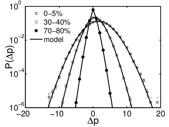
| centrality | |||
|---|---|---|---|
| 0-5% | 351.4 | 14.5 | 1.65 |
| 30-40% | 114.2 | 5.5 | 0.632 |
| 70-80% | 13.4 | 0.83 | 0.075 |
To make predictions for the net-proton distributions at other centralities, one can parameterize the values of parameters and tabulated in TABLE 1 by polynomials of the number of participants as
| (7) | |||||
| (8) |
From this parameterization, one can calculate the moments for the distributions easily. The obtained moments are shown, as functions of the number of participants , in Figs. 2-5. The corresponding experimental data from [6] are shown in the figures for comparison. The calculated mean, variance, skewness and kurtosis are well in agreement with the data. The good agreement shows that the basic merits for the baryon production mechanism have been exhibited in our model consideration.


In Ref. [10], the observed moments are related to the ones from one emission source by using the central limit theorem. This expectation is deduced from the independent emission of particles from each source. In fact, if the baryons are produced from identical sources, one can get relations of the moments for the measured distributions and those for the emission sources as
where quantities with subscript are for moments from one emission source. From the above expressions on centrality dependence, one can expect constant and for all . In our fitting with a single emission source, both changes strongly with centrality. As a result of the centrality dependence of and , the centrality dependence of the moments are well reproduced, as can be seen from Figs. 2-5. One can also calculate moment products and . The centrality dependence of the products are shown in Fig. 6. In the range shown, increases a few percent, while is almost exactly 1, as expected from the hadron resonance gas model [15].

With the good agreement with STAR data at RHIC energy at hand, one can go one step further to predict the higher order moments of the net-proton distributions at LHC energies. For specific, let the center-of-mass energy of the colliding nucleon-nucleon pair be 2.76TeV. From fitting data in [6] one can find the center-of-mass energy dependence of the parameter and extrapolate to LHC/ALICE energy. In this way, one gets at TeV. To get the parameter at LHC/ALICE, one can write , with being the effective emission temperature of the sources and the mass of proton. In [18] the effective temperature of the medium is given as a function of the center-of-mass energy as
with MeV. At LHC, the center of mass energy is much higher than at RHIC, so the value of parameter is much smaller than obtained in the above. The smaller value of will allow more baryon pairs to be produced from a source. The predicted moments are shown in Fig. 7. Now the mean value of the distribution is zero. Because of zero mean value, the net-proton distribution at LHC/ALICE is symmetric about 0 and one gets zero value for the skewness. Since the kurtosis is zero for Gaussian distributions, extremely small value at large at LHC energies means that the net-proton distributions at LHC energies can be well parameterized by Gaussian, but not for small .

IV Conclusion
The higher order moments of the net-proton distributions in relativistic Au+Au collisions at are studied from a simple model with effects from initial baryon stopping and final baryon pair emission taken into account. We have demonstrated that by employing a single emission source model, the distributions at different collision centralities can be well reproduced. Then the higher order moments for the distributions can be calculated without new free parameters. The calculated moments agree well with the experimental results. The predicted moments for LHC Pb+Pb collisions need to be verified experimentally.
It should be mentioned that nothing else is assumed in this model except an initial net-proton and a finite probability for producing baryon pairs from sources. Therefore, our model has nothing to do with thermal equilibrium and/or critical fluctuations. Because our model consideration is based on normal physics effects, our results can be used as a baseline for detecting novel physics in the processes.
Acknowledgements.
This work was supported in part by the National Natural Science Foundation of China under Grant No. 11075061 and by the Programme of Introducing Talents of Discipline to Universities under No. B08033. The authors thank Dr. X.F. Luo for sending us the experimental data. We are grateful to N. Xu and X.F. Luo for valuable discussions.References
- [1] Y. Aoki et al., Nature 443, 675 (2006); M. Cheng et al., Phys. Rev. D 74, 054507 (2006).
- [2] J. Berges, K. Rajagopal, Nucl. Phys. B 538, 215 (1999).
- [3] M. Stephanov, K. Rajagopal and E. Shuryak, Phys. Rev. D 60, 114028 (1999).
- [4] M.A. Stephanov,K. Rajagopal and E.V. Shuryak, Phys. Rev. Lett. 81, 4816 (1998); S. Jeon, V. Koch, Phys. Rev. Lett. 85, 2076 (2000); M. Asakawa, U.W. Heinz and B. Müller, Nucl. Phys. A 698, 519 (2002); V. Koch, J. Phys. G 35, 104030 (2008).
- [5] S. Ejiri, F. Karsch and K. Redlich, Phys. Lett. B 633, 275 (2006).
- [6] M.M. Aggarwal et al., (STAR Collaboration), Phys. Rev. Lett. 105, 022302 (2010).
- [7] S. Gupta et al., Science 332, 1525 (2011); X.F. Luo, B. Mohanty, H.G. Ritter and N. Xu, arXiv:1105.5049.
- [8] F. Karsh and K. Redlich, Phys. Lett. B 693, 136 (2011); M. A. Stephanov, arXiv:1104.1627v1; B. Friman et al., arXiv:1103.3511.
- [9] Y. Zhou et al., Phys. Rev. C 82, 014905 (2010); K. Xiao et al., Chin. Phys. C 35, 467 (2011).
- [10] X.F. Luo, B. Mohanty, H.G. Ritter and N. Xu, arXiv:1001.2847.
- [11] Y. Hatta and M.A. Stephanov, Phys. Rev. Lett. 91, 102003 (2003).
- [12] M.A. Stephanov, Phys. Rev. Lett. 102, 032301 (2009).
- [13] X.F. Luo et al., J. Phys.G 37, 094061 (2010).
- [14] F. Karch and K. Redlich, Phys. Lett. B 695, 136 (2011).
- [15] P. Braun-Munzinger, K. Redlich and J. Stachel, nucl-th/0304013; A. Andronic, P. Braun-Munzinger and J. Stachel, Nucl. Phys. A 772, 167 (2006).
- [16] L.Z. Chen et al., arXiv:1011.0712.
- [17] V.V. Begun et al., Phys. Rev. C 70, 034901 (2004).
- [18] A. Andronic et al., arXiv:1106.6321v1.