Fluctuating hydrodynamics in a vertically vibrated granular fluid with gravity
Abstract
We investigate hydrodynamic fluctuations in a granular fluid excited by a vibrating base and in the presence of gravity, focusing on the transverse velocity modes. Since the system is inhomogeneous, we measure fluctuations in horizontal layers whose width is smaller than the characteristic hydrodynamic lengths: they can be considered as almost-homogeneous subsystems. The large time decay of autocorrelations of modes is exponential and compatible with vorticity diffusion due to shear viscosity, as in equilibrium fluids. The velocity structure factor, which strongly deviates from the equilibrium constant behavior, is well reproduced by an effective fluctuating hydrodynamics described by two noise terms: the first associated with vorticity diffusion and the second with the local energy exchange, which have internal and external character, respectively.
pacs
45.70.-n,05.40.-aI Introduction
Granular systems are ubiquitous on Earth: understanding those materials is essential for the optimization of a variety of industrial processes in the pharmaceutical, food, cosmetic, chemical, petroleum, polymer and ceramic industries [1, 2], it is also propaedeutic for modeling geophysical phenomena such as sediment fluidization in sudden landslides [3, 4, 5] and soil mechanics [6]. Finally, it provides to be a challenge for the statistical physics of out-of-equilibrium complex materials [7, 8, 9, 10, 11]. Fluctuations in granular media are usually non-negligible because of their inherently “small” nature: they are usually composed of a few thousands particles, sometimes even less. On the other side equilibrium statistical mechanics, which is equipped with tools to describe large scale fluctuations of finite systems [12], is not adequate for systems with non-conservative interactions, such as granular fluids undergoing inelastic collisions. A deep understanding of the single-particle velocity fluctuations has been obtained in recent years, through the study of the granular Boltzmann equation and the introduction of several effective models [13, 14, 15, 16]. Fluctuations involving more than one degree of freedom, i.e. correlations, are instead less understood: the reason is that they not always have an equilibrium counterpart. For instance, velocity correlations are ruled out in homogeneous steady elastic fluids, while they play an important role in homogeneous steady inelastic gases [17, 18, 19, 20]. Important progresses on the study of velocity correlations have been achieved for hydrodynamic (i.e. “slow”) modes, in situations where a good separation of length and time scales is observed. While phenomenological fluctuating hydrodynamics has been used in the first study of velocity correlations in homogeneous granular gases [17], a more rigorous treatment through projection formalism from microscopic models has been recently obtained [21]. One of the main results, seen both in the theory and in simulations [22, 23], is that the hydrodynamic noise is not white and does not satisfy the second kind Fluctuation-Dissipation Relation (FDR). These two deviations from the equilibrium fluctuating hydrodynamics are observable but, however, relatively small in homogeneous systems. On the other side, a certain sensitivity to the particular modelling of energy injection has been observed [24, 25]. It is therefore tempting to extend this study to more realistic energy injection models, with the objective of providing a framework for future experiments and more formal analytical treatment. Here, in particular, we are interested in simulating a typical experimental setup, that is a 2D vertical box, under gravity, whose vibrating base acts as a thermal reservoir [26, 27, 24, 28]. The loss of kinetic energy, due to inelastic collisions in the bulk, is counterbalanced by the random floor vibration which injects energy to particles bouncing on it. This setup, which has received careful hydrodynamic treatment [26], is characterized by non-constant density and temperature profiles and by a steady (inhomogeneous) heat flux [29], carrying energy from the bottom region up to the top one. Our analysis, which is purely numerical, focuses on the velocity fields, which is zero on average, provided that convection rolls are not present in the system [30, 31]. Fluctuations of the shear modes (vertical velocity modulated in the horizontal direction at wavelength ) are measured in subsystems small enough to be considered “homogeneous”: a subsystem here is a horizontal layer taking the full width of the system and a fraction of its height, smaller than the smaller characteristic length of hydrodynamic profiles. Three main characterizations of these fluctuations are in order: a) the large time decay of their autocorrelation ; b) the dependence of with , which is a constant for equilibrium fluids, and it is not in non-equilibrium ones; c) the relation between the two previous quantities, which at equilibrium is established in a simple form by the FDR. Previously, fluctuations have been studied in this particular “setup” focusing on other quantities. In [27] single particle velocity fluctuations and density correlations at different height have been studied. In [24] the fluctuations of the total kinetic energy have been investigated, showing that strong non-Gaussian behavior is not due to strong correlations but can be simply accounted by considering inhomogeneous temperature and local Gaussian velocity distributions. This consideration led us to the choice of studying sub-regions of the whole system where homogeneity can be assumed and velocity distributions are not far from the Gaussian. The drawback of this choice is, of course, that each sub-region is an open system and this fact must be taken into account. In Section II we define the model, the simulation scheme and the quantities under study. In Section III the separation of the inhomogeneous system into nearly homogeneous sub-systems is detailed. In Section IV we discuss the numerical results for the points a, b and c described above. In Section V we draw some conclusion and discuss perspectives.
II Model and quantities under study
We perform Molecular Dynamics simulations of inelastic hard disks of diameter and mass , enclosed in a rectangular volume of width and height , under the presence of gravity (pointing in the direction) with acceleration . The energy is injected to the system by a thermal base: this means that a particle colliding with the wall at is bounced back with its velocity component extracted by a Gaussian distribution with temperature and with its velocity component extracted with the distribution [32]
| (1) |
The ceiling of the box is elastically reflecting. Periodic boundary conditions in the direction are adopted. The disks collide inelastically with usual rule dictating the instantaneous velocity change of particle after a collision with particle :
| (2) |
where is the restitution coefficient ( for elastic systems) and is the unit vector joining the colliding disks. We are interested in measuring the velocity shear mode, modulated along the direction, which is the only one where periodic boundary conditions are enforced. This fluctuating variable with complex values is defined as
| (3) |
where is the wave number of chosen mode, the total number of particles and is the
-coordinate of particle at time .
The main
function under investigation is the rescaled autocorrelation of mode
:
| (4) |
measured in the steady state, where and is the “granular temperature” in the direction, with being or . Note that in the region of interest (which includes most of the system, excluding the boundary layers near the bottom and top walls). We will also use the shorthand notation and for the largest mode . In particular we will inspect two main features of the above correlation function, i.e.:
- •
its large time decay, focusing on the dependence on the parameters such as the granular temperature and the particle density and on the wave number ;
- •
the variance of the fluctuations of the modes as a function of , , which is nothing else than the rescaled velocity structure factor; that quantity gives information about the spatial extent of velocity correlations.
Since the fluid receives energy from a boundary and gravity is present, all hydrodynamic profiles are inhomogeneous. In order to avoid the mixing of information coming from regions with different densities and temperatures, in the following section we discuss how to define sub-systems which can be assumed to be nearly homogeneous for our purposes. Before doing that, however, we discuss what is expected in previously studied homogeneous systems.
II.0.1 Behavior of a homogeneous system
For comparison, we briefly review the behavior of the above quantities in an equilibrium homogeneous 2D system and in a granular system both in the homogeneous cooling regime and in the homogeneous stationary state due to uniform random driving.
At equilibrium (at temperature ), the Landau-Lifshitz fluctuating hydrodynamics, based on Einstein fluctuation formula, predicts a Langevin equation for the hydrodynamic shear modes of the kind
| (5) |
where is the kinematic viscosity and is a white noise with zero average and
| (6) |
Based on this equation, one has
| (7) |
In the inelastic homogeneous cooling regime, which is also dilute, the amplitude of fluctuations is decaying: indeed, because of cooling, the kinematic viscosity and decrease with time. In these systems can be written, in the first Sonine approximation, as
| (8) |
where is the equilibrium value of the pair-correlation function, is proportional to the mean free path
and the coefficient is a function of the restitution
coefficient only (see [21] for details).
For that reason
one uses a new time-scale which is proportional to the
cumulative number of collisions [33]: under this new
time-scale the system reaches a stationary regime. Rigorous treatment
from a fluctuating Boltzmann equation in this regime
yields [21]
| (9) |
where
| (10) |
is the cooling rate (see [33] for a definition). The noise results to be non-white, with a correlation
| (11) |
with a function which is given in details in [21]. The steady autocorrelation obtained from the above Langevin equation is not a simple exponential; anyway it has an exponential tail at large times. In particular one obtains
| (12) | ||||
| (13) |
where the two new coefficients and (the latter is usually smaller than the first) are computed in [21]. In the elastic limit , and and result (7) is recovered. In the inelastic case () one immediately sees that the theory is limited to large enough to have : modes with smaller wavenumbers are unstable. That condition obliges to consider systems smaller than a critical size to avoid the instability.
Finally, we consider the case of a homogeneously driven granular gas, as described in [18], where the hydrodynamics of a gas of inelastic grains which receive energy by random uncorrelated velocity kicks is studied. In that work hydrodynamic fluctuations are described using an effective noise that is the sum of an internal and an external noise. The former is originated from the rapid fluctuations of microscopic degrees of freedom and its strength can be obtained from an FDR with respect to internal relaxation. The latter, instead, is due to the random accelerations received by particles from the external driving. The strength of this noise is such that, in the steady state, it balances the energy loss due to the collisions. The result for the shear mode with small inelasticity is a Langevin equation:
| (14) |
with
| (15) |
The corresponding autocorrelation is written as
| (16) |
We stress that other models exist to get a spatially homogeneous and
stationary granular gas, for instance an important modification of the
last one is that introduced in [16], where all particles
feel the presence of a viscous bath: the fluctuating hydrodynamics for
such a model has been recently studied [34] and demonstrated
to fairly describe the experimental behavior of a quasi-2D system on a
horizontal vibrating plate.
An important property common to
all the systems discussed above is the presence of spatial and
thermal homogeneity that is, instead, absent in our system. We
mention that fluctuating hydrodynamics in molecular (elastic) fluids
where a non-equilibrium stationary state is obtained by imposing
(temperature or density) gradients has been studied in the
literature, see for instance [35, 36]. In particular,
in [35] the authors analyze the fluctuations of a fluid under
a stationary heat flux in the presence of a gravity field. They show
that, for small temperature gradients, such system can be studied
within a Landau-Lifshitz approach postulating that FDR still holds
locally. This implies that the transverse velocity modes are well
described by Eq. (5) where all parameters and
coefficients take their local (position-dependent) value, and
therefore do not display any correlation, yielding a flat structure factor.
In the following we will see that the hydrodynamic fluctuations of the granular setup considered here, which is a nearly homogeneous sub-system belonging to a inhomogeneous one, are, for some aspects, well reproduced by a model similar to Eq. (14).
III Quasi-homogeneous sub-systems
The main external parameters influencing the regime are, besides the dimensions of the box, the number of particles, the floor temperature and the restitution coefficient . To give a flavour of the regime we are working on, in Fig. 1 we represent two typical configurations of particle positions in the system from simulations with different restitution coefficients. To fix ideas, useful for the following discussion, we now focus on a particular choice of parameters. The system has height and width , the number of particles is (corresponding to a number of resting layers ), and the restitution coefficient is . Gravity acceleration is set to , while .

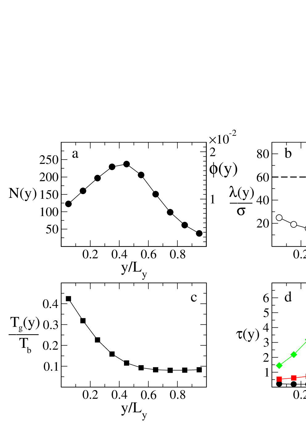
In Figure 2 the behavior of the main “local” observables is reported versus the distance from the floor. We have divided the total height into horizontal layers of height , so that . In each layer (whose height is measured at its middle point) we have computed the average of some observable which is expected to be slowly varying, i.e. the number of particles in the layer and the average kinetic energy in that layer , which are directly associated to the density and temperature hydrodynamic fields [37]. In Figures 2a and 2c we show and respectively. In Fig. 2a one can also appreciate (see right scale) the local packing fraction where is the local density. We also give further information to assess the granular regime chosen for our study. In Figure 2b we report the behavior of the local mean free path (note that is proportional to the local mean free path through a order geometrical factor and through the Enskog constant which, in our dilute case, is very close to ). Finally in Fig. 2d some local characteristic times are reported for the different layers: is the mean collision time, is the mean exit time from the layer with equal to the local thermal velocity and is the time associated to vorticity diffusion obtained from the expectation for the local kinematic viscosity , taken from the granular Enskog theory [37]. These times will be useful (and will be explained in detail) in the discussion of Section IV.
We have verified that the choice of the system parameters as well as the choice of meet the following constraints:
- •
Stability of horizontal modes: if the system is too large it is known that instabilities can arise, starting with shear modes and then involving clustering [38, 17]; a minimum criterion to avoid that is enforcing with the zero-th order approximation of the homogeneous cooling rate in a layer, and the kinematic viscosity in the layer; because this condition determines a constraint on the maximum number of the particles in each layer.
- •
Absence of convection rolls: it is known that this granular setup is also subject to thermal convection instability due to the competition between gravity and temperature gradients [30, 39]; by direct inspection of the velocity field and the dynamical evolution of the numerical simulation we have verified that no convection is present in our system.
- •
Fast local relaxation of microscopic modes: this condition is equivalent to ask that a particle in a layer suffers many collisions before going out from the layer, which (in view of the fact that ) is equivalent to (note that this is not strictly verified in the topmost layer).
- •
Diluteness: to avoid strong velocity correlations and hope a reasonable comparison with dilute hydrodynamic granular theories, we also require that the local packing fraction is small, i.e. .
- •
Local homogeneity: finally, a major constraint in the choice of is given by “quasi-homogeneity” inside the -th layer, i.e. we require that , being one of the “slow” variables, i.e. or .
After having checked by direct inspection that all these requirements are satisfied in our system and with this choice of , we have to warn the reader about two important properties which distinguish this one with respect to other setups, where fluctuating hydrodynamics has been previously discussed (e.g. the homogeneous cooling state [22]). Each horizontal layer is considered here as a single finite system where the fluctuations of velocity shear mode is studied. Anyway:
- 1.
Each layer is an open system, exchanging particles with adjacent layers; we will discuss how this peculiarity do affect the studied fluctuations, in particular the autocorrelation decay.
- 2.
Tuning the external parameters, such as , the total number of particles or the parameters of the thermal base , affects the properties of each layer, e.g. local density or temperature, in a complicate and not direct way. Even if solutions of the hydrodynamic equations for this particular setup exist [26], the boundary layer near the thermal base always requires a careful treatment and makes quantitative predictions for local variables, from the only knowledge of external parameters, quite hard.
IV Numerical results for hydrodynamic fluctuations
IV.1 Time decay of the autocorrelation and dependence on wave number
The behavior of obtained in layers at different height , from the simulations, is shown in Fig. 3a. The autocorrelation function of the shear mode presents two main regimes: a first rapid decay toward an intermediate plateau and a second decay to zero, which is roughly exponential.

Our interpretation of the first decay is that it is associated to the openness of the layer: particles belonging to the layer at time escape from it with a typical velocity , being on average replaced by particles coming from the adjacent layers. In Fig. 3b we have rescaled the time with , getting a fair collapse of the first decay in different layers. This collapse confirms that the typical time of this first decay is and that this is associated to the exchange of particles through the boundaries of the layer. The second decay can be reasonably fit by an exponential law. This fit works better in the central layers, i.e. . Problems in the top and bottom regions could be related to the mean free path becoming too large (this is particularly true in the top region, where it gets closer to the width of the box): in that cases the mean free time could become close to the time taken by a sound wave to travel along the width of the system, producing non-exponential relaxation which could also be size-dependent. The region near the base is also affected by the complicate boundary layer where particles take an asymmetrically distributed vertical velocity because of the thermostat. From now on we focus on the central layers where the decay is well fit by .

In those cases, it is interesting to study the decay time as a function of and to compare it with the theoretical prediction associated to vorticity diffusion which describes the decay of shear modes autocorrelation in a homogeneous elastic system with the viscosity of the layer (see Eq. (8)). To this aim we have performed some simulations modifying only the horizontal size of the box and maintaining the total density constant. In this way we can obtain a better resolution in . Our analysis is focalized to the total density (the same of Fig. 2 and Fig. 3) and and the comparison is shown in Fig. 4. Our first observation is that all data, appropriately rescaled, collapse indicating the same dependence on the local parameters and as the homogeneous system. In particular, data in the range show a very good agreement with the prediction of simple vorticity diffusion due to shear viscosity . From values , shows deviations from : we suspect that this is an indication of the failure of the hydrodynamical approach at such small lengthscales. A less clear failure is present also at very large wavelengths (): such a discrepancy suggests the presence of some mechanism slowing the relaxation of shear modes, perhaps a precursor of power-law relaxation associated to the two-dimensional geometry.
IV.2 Structure factor of transverse velocity modes
The amplitude of fluctuations of the shear mode in a layer, which is directly proportional to the transverse velocity structure factor, is given (see Eq.(3)) by
| (17) |
From Eq. (17) it is seen that can be split into two parts: a first self term which scales as and a second term, that contains the informations of the -dependence in a layer at height .

In a homogeneous equilibrium fluid, from equilibrium statistical mechanics, one expects the absence of spatial velocity correlations, corresponding to a flat , as expressed by Eq. (7). Homogeneously cooling granular systems (with size smaller than the critical size for linear stability of shear modes) are expected to present a non-flat structure factor, implying spatial velocity correlations, as marked by Eq. (12). However those systems present an instability which is not directly observed in our simulations (unless one gets much larger horizontal size ). Moreover, our layer is in a stationary state, a regime quite different from the cooling state: such a difference is reasonable because each layer is “driven” by particles coming from nearby layers. The best candidate as a model for quantitative comparison with our numerical results is the homogeneously driven system studied in [18], whose fluctuating hydrodynamics we have resumed in Eq. (14). Our system is different from that model, since we have not a uniform noise throughout the system, but the addition of energy is localized at the bottom of the box. Nevertheless in a single layer there is a balance between the energy exchanged with adjacent layers and the energy dissipated in collisions. It is therefore tempting to introduce an effective external noise whose amplitude is determined by the energy balance and is proportional to . Using this expression for noise and considering that the characteristic decay time is , the quantity can be written as
| (18) |
Comparing Eqs. (17) and (18) we note that can be written as . In an elastic homogeneous system this term is zero, while in a granular system we observe a non-negligible contribute of . In order to verify our assumption we have plotted in Fig. 5 the simulation data for and its prediction based on the Eq. (18) and estimated using for the data plotted in Fig. 4. The agreement is very good for both the cases analyzed (open and closed symbols in Fig. 5) and this validates our considerations. Moreover we have verified that the probability distribution of is close to a Gaussian, consistent with a linear Langevin equation. In Fig. 5 only results from the central layer () are shown: however we have verified that it is equally good in the contiguous layers. For the sake of completeness we have shown in the figure also obtained using as characteristic time . The disagreement is small and analogous to that already seen in the previous section.
IV.3 Amplitude of fluctuations for the mode at largest wavelength
To have a better assessment of our hypothesis (Eq. (18)), we
focus now on the amplitude of the shear mode
for the largest available wavelength . Indeed one expects
that at larger wavelengths hydrodynamics works better. For such a
purpose, we have fixed the width () and we have
changed the total number of the particles. In this way the local
density is also changed and we can explore the dependence of
on the particle number or,
equally, on .

Measures of for many different layers and for systems with three values of the restitution coefficient (, and ) are shown in in Fig. 6a. The data are rescaled by the factor because this term contains the main dependence on in the Eq. (18). The collapse of data is quite remarkable, if one consider that data come from different systems and from layers which can be at very different distance from the base: for instance, a given value of can correspond both to layers below the density maximum and above it. At moderate values of the data are closed to the values obtained using as decay time in Eq. (18). The disagreement at small values of is due to the fact that hydrodynamic hypothesis is not longer valid in this range. It is likely that the deviations from a clean collapse in Fig. 6a are due to the mixing of data from regions characterized by too different physical parameters as and . We have repeated the analysis by focusing only on the layer containing the maximum of the density , but changing the external parameters in order to explore different values of . The corresponding value is presented in Fig. 6b. The data do not rescale exactly and this indicates an uncleared dependence. On the other side the measures are in good agreement with the corresponding data obtained from Eq. (18) (open symbols in figure). This suggests that the Eq. (18 ) reproduces the right behavior provided that the suitable decay time is used. Concerning this point, it is important to notice that for large values of , (or ) can become much larger than that observed in the homogeneous cooling state (see dashed line in Fig. 6).
V Conclusions
We have analyzed the fluctuations of the shear mode of the velocity in
nearly homogeneous subregions of a inhomogeneous granular fluid. Our
conclusion is that - neglecting regions too close to the upper and
lower boundaries - the large time temporal decay of their
autocorrelation does not deviate dramatically from the expectation for
a homogeneous equilibrium fluid, i.e. , provided that
hydrodynamic (large enough) scales are considered. At too large
scales, comparable with the total horizontal size, some deviations
from the behavior is appreciated, likely due to finite
size effects and problems associated to the 2D geometry.
The study
of the amplitude of fluctuations, i.e. the transverse velocity
structure factor, suggests that for the central layers, the effective
noise is well described by a sum of two contributions, both white and
Gaussian: an internal one, associated to the vorticity current, which
is at “equilibrium” with the local temperature, and an external one
which is responsible for the balance of local energy which is
continuously lost in collisions. We have shown that those assumptions
lead to a good estimate of the structure factor in all cases analyzed,
if the autocorrelation decay time used in the formula is the one
measured in the simulations: such an agreement holds even when the
decay time deviates from the simple prediction .
We
stress that formula (18) for the amplitude of fluctuations
represents an explicit violation of the equilibrium
Fluctuation-Dissipation Relation, which would yield a constant
structure factor: such a violation can be quite large with respect to
those discussed in the homogeneous cooling regime [22]. In
particular, violations observed here lead to an amplitude of
fluctuations which can be much larger than that expected at
equilibrium or in the homogeneous cooling theory. It is also
remarkable to notice that the correlations observed here are not
related to the gradients in the system (as it happens for other
correlations in molecular systems with an imposed thermal or density
gradient), but are a direct consequence of inelastic collisions.
Acknowledgments
We acknowledge Prof. U. Marini Bettolo Marconi and Dr. G. Gradenigo for useful discussions and a critical reading of the manuscript. The work of the authors is supported by the “Granular-Chaos” project, funded by the Italian MIUR under the FIRB-IDEAS grant number RBID08Z9JE.
References
- [1] J. Duran, Sands, powders, and grains: an introduction to the physics of granular materials (Springer-Verlag, New-York, 2000).
- [2] H. M. Jaeger, S. R. Nagel, and R. P. Behringer, Reviews of Modern Physics 68, 1259 (1996).
- [3] C. H. Scholz, Nature 391, 37 (1998).
- [4] R. M. Iverson, Rev. Geophys. 35, 245 (1997).
- [5] P. A. Johnson and X. Jia, Nature 437, 871 (2005).
- [6] A. Khaldoun, E. Eiser, G. H. Wegdam, and D. Bonn, Nature 437, 635 (2005).
- [7] L. P. Kadanoff, Rev. Mod. Phys. 71, 435 (1999).
- [8] A. Kudrolli, Nature Materials 7, 174 (2008).
- [9] E. R. Nowak, J. B. Knight, M. L. Povinelli, H. M. Jaeger, and S. R. Nagel, Powder Technology 94, 79 (1997).
- [10] G. Biroli, Nature Physics 3, 222 (2007).
- [11] A. S. Keys, A. R. Abate, S. C. Glotzer, and D. J. Durian, Nature Physics 3, 260 (2007).
- [12] L. D. Landau and E. M. Lifchitz, Physique Statistique (Éditions MIR, 1967).
- [13] S. E. Esipov and T. Pöschel, J. Stat. Phys. 86, 1385 (1997).
- [14] T. P. C. van Noije and M. H. Ernst, Granular Matter 1, 57 (1998).
- [15] D. R. M. Williams and F. C. MacKintosh, Phys. Rev. E 54, R9 (1996).
- [16] A. Puglisi, V. Loreto, U. M. B. Marconi, A. Petri, and A. Vulpiani, Phys. Rev. Lett. 81, 3848 (1998).
- [17] T. P. C. van Noije, M. H. Ernst, R. Brito, and J. A. G. Orza, Phys. Rev. Lett. 79, 411 (1997).
- [18] T. P. C. van Noije, M. H. Ernst, E. Trizac, and I. Pagonabarraga, Phys. Rev. E 59, 4326 (1999).
- [19] I. Pagonabarraga, E. Trizac, T. P. C. van Noije, and M. H. Ernst, Phys. Rev. E 65, 011303 (2001).
- [20] A. Baldassarri, U. M. B. Marconi, and A. Puglisi, Phys. Rev. E 65, 051301 (2002).
- [21] J. J. Brey, P. Maynar, and M. I. Garcia de Soria, Phys. Rev. E 79, 051305 (2009).
- [22] J. J. Brey, M. I. G. de Soria, and P. Maynar, Europhys. Lett. 84, 24002 (2008).
- [23] G. Costantini and A. Puglisi, Phys. Rev. E 82, 011305 (2010).
- [24] P. Visco, A. Puglisi, A. Barrat, F. van Wijland, and E. Trizac, Eur. Phys. J. B 51, 377 (2006).
- [25] P. Maynar, M. de Soria, and E. Trizac, Eur. Phys. J. Special Topics 179, 123 (2009).
- [26] J. J. Brey, M. J. Ruiz-Montero, and F. Moreno, Phys. Rev. E 63, 061305 (2001).
- [27] A. Baldassarri, U. Marini Bettolo Marconi, A. Puglisi, and A. Vulpiani, Phys. Rev. E 64, 011301 (2001).
- [28] D. Paolotti, C. Cattuto, U. M. B. Marconi, and A. Puglisi, Granular Matter 5, 75 (2003).
- [29] J. J. Brey and M. J. Ruiz-Montero, Europhys. Lett. 66, 805 (2004).
- [30] R. Ramírez, D. Risso, and P. Cordero, Phys. Rev. Lett. 85, 1230 (2000).
- [31] D. Paolotti, A. Barrat, U. Marini Bettolo Marconi, and A. Puglisi, Phys. Rev. E 69, 061304 (2004).
- [32] R. Tehver, F. Toigo, J. Koplik, and J. R. Banavar, Phys. Rev. E 57, R17 (1998).
- [33] J. J. Brey, M. J. Ruiz-Montero, and F. Moreno, Phys. Rev. E 69, 051303 (2004).
- [34] G. Gradenigo, A. Sarracino, D. Villamaina, and A. Puglisi, arxiv:1103.0166 (2011).
- [35] R. Schmitz and E. G. D. Cohen, J. Stat Phys. 39, 285 (1985).
- [36] J. M. O. de Zárate and J. V. Sengers, Hydrodynamic fluctuations in fluids and fluid mixtures (Elsevier, Amsterdam, 2006).
- [37] J. J. Brey, J. W. Dufty, C. S. Kim, and A. Santos, Phys. Rev. E 58, 4638 (1998).
- [38] I. Goldhirsch and G. Zanetti, Phys. Rev. Lett. 70, 1619 (1993).
- [39] R. D. Wildman, J. M. Huntley, and D. J. Parker, Phys. Rev. Lett. 86, 3304 (2001).