Non-adaptive probabilistic group testing with noisy measurements: Near-optimal bounds with efficient algorithms
Abstract
We consider the problem of detecting a small subset of defective items from a large set via non-adaptive “random pooling” group tests. We consider both the case when the measurements are noiseless, and the case when the measurements are noisy (the outcome of each group test may be independently faulty with probability ). Order-optimal results for these scenarios are known in the literature. We give information-theoretic lower bounds on the query complexity of these problems, and provide corresponding computationally efficient algorithms that match the lower bounds up to a constant factor. To the best of our knowledge this work is the first to explicitly estimate such a constant that characterizes the gap between the upper and lower bounds for these problems.
I Introduction
The goal of group testing is to identify a small unknown subset of defective items embedded in a much larger set (usually in the setting where is much smaller than , i.e., is ). This problem was first considered by Dorfman [1] in scenarios where multiple items in a group can be simultaneously tested, with a binary output depending on whether or not a “defective” item is presented in the group being tested. In general, the goal of group testing algorithms is to identify the defective set with as few measurements as possible. As demonstrated in [1] and future work, with judicious grouping and testing, far fewer than the trivial upper bound of may be required to identify the set of defective items.
In this work our model has four important assumptions.
- •
Non-adaptive group testing: The set of items being tested in each test is required to be independent of the outcome of every other test. This restriction is often useful in practice, since this enables parallelization of the testing process. It also allows for an automated testing process (whereas the procedures and especially the hardware required for adaptive group testing may be significantly more complex). Furthermore, it is known (for instance [2], [3]) that adaptive group testing algorithms do not improve upon non-adaptive group-testing algorithms by more than a constant factor in the number of tests required to identify the set of defective items.
- •
“Small-error” group testing: Our algorithms are allowed to have a “small” probability of error. It is known (for instance [3]) that zero-error algorithms require significantly more tests asymptotically (in the number of defective items) than algorithms that allow asymptotically small errors.
- •
“Noisy” measurements: In addition to the noiseless group-testing problem specified by the above, we also consider the “noisy” variant of the problem, wherein the result of each test may differ from the true result (in an independent and identically distributed manner) with a certain pre-specified probability . 11 1 An alternative model involving “worst-case” errors has also been considered in the literature (for instance [4]), wherein the designed group-testing algorithm is required to be resilient to all noise patterns wherein at most a fraction of the results differ from their true values, rather than the probabilistic guarantee we give against most fraction- errors. This is analogous to the difference between combinatorial coding-theoretic error-correcting codes (for instance Gilbert-Varshamov codes [5]) and probabilistic information-theoretic codes (for instance [6]). In this work we concern ourselves only with the latter, though it is possible that our techniques can also be used to analyzed the former. Since the measurements are noisy, the problem of estimating the set of defective items is more challenging, and is known to require more tests. 22 2 We wish to highlight the difference between noise and errors. We use the former term to refer to noise in the outcomes of the group-test, regardless of the group-testing algorithm used. The latter term is used to refer to the error due to the estimation process of the group-testing algorithm.
- •
Computationally efficient and near-optimal algorithms: Most algorithms in the literature focus on optimizing the number of measurements required – in some cases, this leads to algorithms that may not be computationally efficient to implement (for e.g. [3]). In our work we require our algorithms be both computationally efficient and near-optimal in the number of measurements required.
In the literature, order-optimal upper and lower bounds on the number of tests required are known for the problems we consider (for instance [3], [7]). In both the noiseless and noisy variants, the number of measurements required to identify the set of defective items is known to be – here is the total number of items and is the size of the defective subset. However, in the noisy variant, the number of tests required is in general a constant factor larger than in the noiseless case (where this constant is independent of both and , but may depend on the noise parameter and the allowable error-probability of the algorithm.
However, to the best of our knowledge, prior to this work no explicit characterization has been given of the actual number of measurements required (rather than just order-optimal results). In particular, we analyze two algorithms that we call Combinatorial Basis Pursuit (CBP), and Combinatorial Orthogonal Matching Pursuit (COMP),33 3 This choice of nomenclature is motivated by two popular Compressive Sensing decoding algorithms, respectively Basis Pursuit, and Orthogonal Matching Pursuit – as we note in Section I-A, the decoding algorithms we analyze in this work might be viewed as combinatorial analogues of those well-analyzed algorithms. that have both been previously considered in the group-testing literature (under different names) for both noiseless and noisy scenarios (see, for instance, [8]). We provide explicit upper bounds on for both these algorithms. Further, we also provide corresponding lower bounds on for any group-testing algorithms. These upper and lower bounds are asymptotically independent of both and . The lower bounds are information-theoretic, and the upper bounds are derived from a detailed analysis of CBP and COMP under both the noiseless and noisy scenarios. In general, the bounds resulting from the analysis of the algorithms match our simulations to a high degree, which indicates that the bounds we derive are not too slack.
This paper is organized as follows. In Section II, we introduce the model and corresponding notation, and describe the algorithms analyzed in this work. In Section III, we describe the main results of this work. Sections IV and V contain the analysis respectively our information-theoretic lower bounds, and of the group-testing algorithms considered. Our simulation results are presented in Section VI.
I-A Prior Work
Dorfman [1] first considered the group-testing problem during World-War II with regards to testing soldiers for syphilis. Since then, a large body of literature has considered the problem (see for instance the book by [2]).
In this work we focus on non-adaptive algorithms. Here we can further subdivide algorithms according to whether errors (that decay asymptotically to zero with large ) are allowed or not in the reconstruction algorithm, and, orthogonally, whether the measurements are noisy are not.
If errors are not allowed in the group-testing algorithm, it is known that at least tests are required in both noiseless and noisy scenarios (which may be considerably larger than the bounds that are known (for instance [3] and [7]) for the ‘‘small-error” scenario. Further, in the noisy scenario, if no errors are allowed in the reconstruction algorithm, only noise patterns with an absolute bound on the total number of noisy measurements can be handled.44 4 This is because in the “usual” noise model, wherein each measurement may be noisy with a certain probability, there is a non-zero probability that an arbitrary fraction of the measurements are corrupted in an arbitrarily bad manner. In this case no group-testing algorithm can hope to decode with zero-error. For these reasons, we choose to focus on algorithms in which a small probability of error is allowed – the reader interested in zero-error algorithms is encouraged to look at [2], [9], [10], [11], [12].
The works closest to ours are those of [3] and [7]. The former analyzes the performance of certain group-testing algorithms in both noiseless and noisy settings information-theoretically, and proves order-optimality. However, only order-optimal (rather than explicit) bounds on the number of tests required are provided, and also the algorithms analyzed are not provided, and also the algorithms analyzed are not computationally efficient. The work of [7] proposes a belief-propogation decoding rule to improve the computational efficiency of the algorithms of [3], but no proof of correctness is provided. In contrast, in this work we provide the first explicit bounds on computationally efficient group-testing algorithms.
Information-theoretic lower bounds on the number of tests required are folklore – some instances of these bounds for some models are provided in [10]. Since we were unable to find a specific reference covering all cases for our model, we also prove our lower bounds in Section IV.
There are intriguing connections between the two algorithms we consider, and corresponding Compressive Sensing (CS) algorithms. In particular, Basis Pursuit has been well-analyzed in the CS literature (for instance [13, 14]), as has Orthogonal Matching Pursuit (for instance [15]). The primary difference between those algorithms and the ones considered here is that in CS all measurements are over the real field , whereas in group-testing the measurements are modeled instead as an OR of AND clauses (hence the term “Combinatorial”).
II Background
II-A Model and Notation

A set contains items, of which an unknown subset are said to be ‘‘defective”.55 5 In this work, as is common (see for example [16]), we assume that the number of defective items in , or at least a good upper bound on them, is known a priori. If not, other work (for example [17]) considers non-adaptive algorithms with low query complexity that help estimate . The goal of group-testing is to correctly identify the set of defective items via a minimal number of “group tests”, as defined below (see Figure 1 for a graphical representation).
Each row of a binary group-testing matrix corresponds to a distinct test, and each column corresponds to a distinct item. Hence the items that comprise the group being tested in the th test are exactly those corresponding to columns containing a in the th location. The method of generating such a matrix is part of the design of the group test – this and the other part, that of estimating the set , is described in Section II-B.
The length- binary input vector represents the set , and contains s exactly in the locations corresponding to the items of . The locations with ones/defective items are said to be positive – the other locations are said to be negative. We use these terms interchangeably.
The outcomes of the noiseless tests correspond to the length- binary noiseless result vector , with a in the location if and only if the th test contains at least one defective item.
The observed vector of test outcomes in the noisy scenario is denoted by the length- binary noisy result vector – the probability that each entry of differs from the corresponding entry in is , where is the noise parameter. The locations where the noiseless and the noisy result vectors differ is denoted by the length- binary noise vector , with s in the locations where they differ.
The estimate of the locations of the defective items is encoded in the length- binary estimate vector, with s in the locations where the group-testing algorithms described in Section II-B estimate the defective items to be.
The probability of error of any group-testing algorithm is defined as the probability (over the input vector , group-testing matrix , and noise vector ) that the estimated vector differs from the input vector.
II-B Algorithms
We now describe the CBP and COMP algorithms in both the noiseless and noisy settings. The algorithms are specified by the choices of encoding matrices and decoding algorithms.
1. NOISELESS ALGORITHMS
Combinatorial Basis Pursuit (CBP):
The group-testing matrix is defined as follows. A group sampling parameter is chosen (the exact values of and are code-design parameters to be specified later). Then, the th row of is specified by sampling with replacement from the set exactly times, and setting the location to be one if is sampled at least once during this process, and zero otherwise.66 6 Note that this process of sampling each item in each test with replacement results in a slightly different distribution than if the group-size of each test was fixed a priori and hence the sampling was “without replacement” in each test. (For instance, in the process we define, each test may, with some probability, test fewer than items.) The “without replacement” process is a perhaps more natural way of defining tests, and also experimentally seems to result in slightly better performing algorithms. However, the corresponding analysis is significantly trickier, and we have been unable to find closed form expressions for such “without replacement” sampling. The primary advantage of analyzing the “with replacement” sampling is that in the resulting group-testing matrix every entry is then chosen i.i.d..
The decoding algorithm proceeds by using only the tests which have a negative (zero) outcome, to identify all the non-defective items, and declaring all other items to be defective. If is chosen to have enough rows (tests), each non-defective test should, with significant probability, appear in at least one negative test, and hence will be appropriately accounted for. Errors (false positives) occur when at least one non-defective item is not tested, or only occurs in positive tests (i.e., every test it occurs in has at least one defective item). The analysis of this type of algorithm comprises of estimating the trade-off between the number of tests and the probability of error.
More formally, for all tests whose measurement outcome is a zero, let denote the corresponding th row of , and denote the length- binary vector which has s in exactly those locations where there is a in at least one . The decoder sets as , i.e., it has zeroes where has ones, and vice versa.
The rough correspondence between this algorithm and Basis Pursuit ([13, 14]) arises from the fact that, as in Basis Pursuit, the decoder attempts to find a “sparse” solution that can generate the observed vector .

Combinatorial Orthogonal Matching Pursuit (COMP):
The group-testing matrix is defined as follows. A group selection parameter is chosen (the exact values of and are code-design parameters to be specified later). Then, i.i.d. for each , the th element of is set to be one with probability , and zero otherwise.
The decoding algorithm columns-wise, instead of row-wise as in CBP. It attempts to match the columns of with the result vector . That is, if a particular column of has the property that all locations where it has ones also corresponds to ones in in the result vector, then the th item () is declared to be defective (positive). All other items are declared to be non-defective (negative).
Note that this decoding algorithm never has false negatives, only false positives. A false positive occurs when all locations with ones in the th column of (corresponding to a non-defective item ) are “hidden” by the ones of other columns corresponding to defectives items. That is, let columns and some other columns of matrix be such that for each such that , there exists an index in for which also equals . Then if each of the th items are defective, then the th item will also always be declared as defective by the COMP decoder, regardless of whether or not it actually is. The probability of this event happening becomes smaller as the number of tests become larger. Hence, as in CBP, the analysis of this type of algorithm comprises of estimating the trade-off between the number of tests and the probability of error.
The rough correspondence between this algorithm and Orthogonal Matching Pursuit ([15]) arises from the fact that, as in Orthogonal Matching Pursuit, the decoder attempts to match the columns of the group-testing matrix with the result vector.

2. NOISY ALGORITHMS
Noisy Combinatorial Basis Pursuit (NCBP):
Let be design parameters to be specified later. To generate the for the NCBP algorithm case, each row of from the noiseless CBP algorithm is repeated times. The decoder declares the result of each a particular set of successive tests to be positive if at least of the tests in that group are positive, and else declares each such test to actually be negative. The decoder then uses the noiseless CBP algorithm to estimate .
Noisy Combinatorial Orthogonal Matching Pursuit (NCOMP)
Finally, we consider the algorithm whose analysis is the major result of this work. In the noisy COMP case, we relax the sharp-threshold requirement in the original COMP algorithm that the set of locations of ones in any column of corresponding to a positive item be entirely contained in the set of locations of ones in the result vector. Instead, we allow for a certain number of “mismatches” – this number of mismatches depends on both the number of ones in each column, and also the noise parameter .
Let and be design parameters to be specified later. To generate the for the NCOMP algorithm case, each element of is selected i.i.d. with probability to be .
The decoder proceeds as follows, For each column , we define the indicator set as the set of indices in that column where . We also define the matching set as the set of indices where both (corresponding to the noisy result vector) and .
Then the decoder uses the following “relaxed” thresholding rule. If , then the decoder declares the th item to be defective, else it declares it to be non-defective.

However, consider the false negative generated for the item in (c). This corresponds to the th item. The noise in the nd, rd and th rows of means that there is only one match (in the th row) and two mismatches (nd and th rows) – hence the decoder declares that item to be non-defective.
Also, sometimes, as in (a), an item that is truly negative, has a sufficient number of measurement errors that the number of mismatches is reduced to be below the threshold, leading to a false positive.
III Main Results
III-A Lower Bounds
We first provide information-theoretic lower bounds on the number of tests required by any group-testing algorithm. While we believe these bounds to be “common knowledge” in the field, we have been unable to pinpoint a reference that gives an explicit lower bound on the number of tests in terms of the acceptable probability of error of the group-testing algorithm. For the sake of completeness, so we can benchmark our analysis of the algorithms we present later, we state and prove the lower bounds here. All logarithms in this work are assumed to be binary.
Theorem 1
[Folklore] Any group-testing algorithm with noiseless measurements that has a probability of error of at most requires at least tests.
In fact, the corresponding lower bounds can be extended to the scenario with noisy measurements as well.
Theorem 2
[Folklore] Any group-testing algorithm that has measurements that are noisy i.i.d. with probability and that has a probability of error of at most requires at least tests.77 7 Here denotes the binary entropy function.
III-B Upper Bounds
The main contributions of this work are explicit computations of the number of tests required to give a desired probability of error via computationally efficient algorithms. In both the noiseless and noisy case, we consider two types of algorithms (CBP and COMP). Both these algorithms have been considered before in the literature (for instance, see [8]), but to the best of our knowledge ours is the first work to explicitly compute the tradeoff between the number of tests required to give a desired probability of error, rather than giving order of magnitude estimates of the number of tests required for a “reasonable” probability of success.
Theorem 3
CBP with error probability at most requires no more than tests.
Theorem 4
COMP with error probability at most requires no more than tests.
Translating these algorithms into the noisy measurement case is non-trivial. One approach is to repeat the tests in CBP, leading to NCBP and the following theorem.
Theorem 5
NCBP with probability of error at most requires no more than tests.
Note that this is asymptotically worse than the corresponding lower bound in Theorem 2. We therefore provide the main result of this paper,
Theorem 6
NCOMP with error probability at most requires no more than tests.
Note that the corresponding upper bound differs from the lower bound by a factor that is at most , which is a function only of and . for “small” this quantity is “small”.
IV Proof of lower bounds
We begin by noting that (i.e. the input vector, noiseless result vector, noisy result vector, and the estimate vector) forms a Markov chain. By standard information-theoretic definitions we have
Since is uniformly distributed over all length- and -sparse data vectors, . By Fano’s inequality, . Also, we have by the data-processing inequality. Finally, note that
since the first term is maximized when each of the are independent, and because the measurement noise is memoryless. For the BSC() noise we consider in this work, this summation is at most by standard arguments.88 8 This technique also holds for more general types of discrete memoryless noise – for ease of presentation, in this work we focus on the simple case of the Binary Symmetric Channel.
Combining the above inequalities, we obtain
Also, by standard arguments via Stirling’s approximation [18], is at least . Substituting this gives us the desired result
V Proofs of upper bounds
V-A Noiseless Group Testing
Proof of Theorem 3:
The Coupon Collector’s Problem (CCP) is a classical problem that considers the following scenario. Suppose there are types of coupons, each of which is equiprobable. A collector selects coupons (with replacement) until he has a coupon of each type. What is the distribution on his stopping time? It is well-known ([19]) that the expected stopping time is . Also, reasonable bounds on the tail of the distribution are also known – for instance, it is known that the probability that the stopping time is more than is at most .
Analogously to the above, we view the group-testing procedure of CBP as a Coupon Collector Problem. Consider the following thought experiment. Suppose we consider any test as a length- test-vector 99 9 Note that this test-vector is different from the binary length- vectors that specify tests in the group testing-matrix, though there is indeed a natural bijection between them. whose entries index the items being tested in that test (in this view, repeated entries are allowed in this vector). Due to the design of our group-testing procedure in CBP, the probability that any item occurs in any location of such a vector is uniform and independent. In fact this property (uniformity and independence of the value of each entry of each test) also holds across tests. Hence, the items in any subsequence of tests may be viewed as the outcome of a process of selecting a single chain of coupons. This is still true even if we restrict ourselves solely to the tests that have a negative outcome. The goal of CBP may now be viewed as the task of collecting all the negative items. This can be summarized in the following equation
| (1) |
Modifying (1) to obtain the corresponding tail bound on takes a bit more work. The right-hand side is then modified to (which corresponds to the probability that all types of coupons have not been collected if these many total coupons have been collected is at most ). The left-hand side is multiplied with , where is a design parameter to be specified by Chernoff’s bound on the probability that the actual number of items in the negative tests is smaller than times the expected number. By Chernoff’s bound this is at most . Taking the union bound over these two low-probability events gives us that the probability that
| (2) |
does not hold is at most
| (3) |
| (4) | |||||
Using the inequality with as simplifies the RHS of (4) to
| (5) |
Choosing to be greater than the bound in (5) can only reduce the probability of error, hence choosing
| (6) |
still implies a probability of error at most as large as in (3).
Choosing and substituting (6) into (3) implies, for large enough , the probability of error satisfies
| (7) | |||||
Taking , we have . For large , approaches .
Therefore, the probability of error is at most , with sufficiently large , the following number of tests suffice to fulfil the terms of the theorem
Proof of Theorem 4:
As noted in the discussion on COMP in Section II-B, the error-events for the algorithm correspond to false positives, when a column of corresponding to a non-defective item is ”hidden” by other columns corresponding to defective items. To calculate this probability, recall that each entry of equals one with probability , i.i.d. Let index a column of corresponding to a non-defective item, and let index the columns of corresponding to defective items. Then the probability that equals one, and at least one of also equals one is . Hence the probability that the th column is hidden by a column corresponding to a defective item is . Taking the union bound over all non-defective items gives us that the probability of false positives is bounded from above by
| (8) |
By differentiation, optimizing (8) with respect to suggests choosing as . Substituting this value back into (8), and setting as gives us
| (9) | |||||
Choosing thus ensures the required decay in the probability of error. Hence choosing to be at least suffices to prove the theorem. .
V-B Noisy Group Testing
We now consider the harder problem of group testing when the measurements are noisy. First, just as a benchmark, we consider using the noiseless CBP algorithm with each test repeated identically times, where is a parameter to be determined so as to ensure a probability of error that can be made to decay asymptotically in .
Proof of Theorem 5:
Since each test has a probability of giving the wrong result, by the Chernoff bound the probability that more than the threshold number of tests give the incorrect result is at most . Hence by the union bound, repeating each of the tests times, the probability that the decoder makes an error is at most
| (10) |
Substituting as implies that for the probability (10) to approach zero asymptotically in must be at least
| (11) | |||||
.
Note: As noted earlier, the number of tests required by NCBP is larger than the corresponding lower bound in Theorem 2 by a factor that is larger than any constant.
Proof of Theorem 6:
Due to the presence of noise, both false positives and false negatives may occur in the noisy COMP algorithm – the overall probability of error is the sum of the probability of false positives and that of false negatives. We set (where is a code-design parameter to be determined later) and . We first calculate the probability of false positives by computing the probability that more than the expected number of ones get flipped to zero in the result vector in locations corresponding to ones in the column indexing the defective item. This can be computed as
| (13) | |||||
| (14) | |||||
| (15) | |||||
| (16) | |||||
| (17) | |||||
| (18) |
Here, as in Section II-B, denotes the locations of ones in the th column of . Inequality (13) follows from the union bound over the possible errors for each of the defective items, with the first summation accounting for the different possible sizes of , and the second summation accounting for the error events corresponding to the number of one-to-zero flips exceeding the threshold chosen by the algorithm. Inequality (14) follows from the Chernoff bound. Equality (15) comes from the binomial theorem. Equality (16) comes from substituting in the values of and . Inequality (17) follows from the leading terms of the Taylor series of the exponential function. Inequality (18) follows from an appropriate linear lower bound to the concave function .
For the requirement that the probability of false negatives be at most to be satisfied implies that (the bound on due to this restriction) be at least . Since this converges to
| (19) |
We now focus on the probability of false positives. In the noiseless CBP algorithm, the only way a false positive could occur was if all the ones in a column are hidden by ones in columns corresponding to defective items. In the noisy CBP algorithm this still happens, but in addition noise could also lead to a similar masking effect. That is, even in the locations of a non-defective column not hidden by other defective columns, measurement noise flips enough zeroes to ones so that the decoding threshold is exceeded, and the decoder declares that particular item to be defective. See Figure 4(a) for an example.
Hence we define a new quantity , which denotes the probability for any th location in that a in that location is “hidden by other columns or by noise”. It equals
To facilitate our analysis, as for , we bound
| (20) | |||||
The probability of false positives is then computed in a similar manner to that of false negatives as in (13)–(18).
| (21) | |||||
| (23) | |||||
Note that for the Chernoff bound to applicable in (21), . Equation (23) follows from substituting the bound derived on in (20) into (21). For the requirement that the probability of false positives be at most to be satisfied implies that (the bound on due to this restriction) be at least . Since this converges to
| (24) |
When the threshold in the noisy COMP algorithm is high (i.e., is small) then the probability of false negatives increases; conversely, the threshold being low ( being large) increases the probability of false positives. Algebraically, this expresses as the condition that (else the probability of false negatives is significant), and conversely to the condition that (so that the Chernoff bound can be used in (21)) – combined with (20) this implies that . For fixed , each of (19) and (24) as a function of is a reciprocal of a parabola, with a pole the corresponding extremal value of . Furthermore, is strictly increasing and is strictly decreasing in the region of valid in . Hence the corresponding curves on the right-hand sides of (19) and (24) intersect within the region of valid , and a good choice for is at the where these two curves intersect. Let
| (25) |
(Note that for large , since , approaches .) Then equating the RHS of (19) and (24) implies that the optimal satisfies
| (26) |
Simplifying (26) gives us that
| (27) |
Substituting (27) into (24) we see that the resulting function can be viewed as times factors that are independent of . Optimizing this with respect to indicates that the minimal value of occurs when .
Substituting these values of , and into (19) gives us the explicit bound
| (28) |
VI Simulation
VI-A Noisy Random Incidence Algorithm
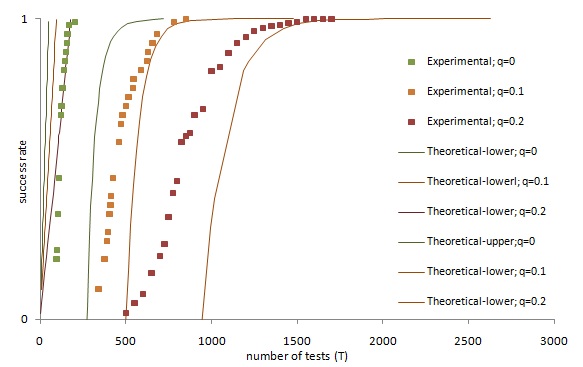
We performed extensive simulations to validate our theoretical analysis. In the interest of space we present only Figure 5, which examines the probability of error of Noisy-COMP as a function of the number of tests. Note that the experimental values we obtain correlate well with the corresponding bounds.
References
- [1] R. Dorfman, “The detection of defective members of large populations,” Annals of Mathematical Statistics, vol. 14, no. 436-411, 1943.
- [2] D.-Z. Du and F. K. Hwang, Combinatorial Group Testing and Its Applications, 2nd ed. World Scientific Publishing Company, 2000.
- [3] G. Atia and V. Saligrama, “Boolean compressed sensing and noisy group testing,” CoRR, vol. abs/0907.1061, 2009.
- [4] A. J. Macula, “Error-correcting nonadaptive group testing with de-disjunct matrices,” Discrete Applied Mathematics, vol. 80, no. 2-3, pp. 217 – 222, 1997.
- [5] E. N. Gilbert, “A comparison of signaling alphabets,” Bell System Technical Journal, vol. 31, pp. 504–522, 1952.
- [6] C. E. Shannon, “A mathematical theory of communication,” SIGMOBILE Mob. Comput. Commun. Rev., vol. 5, pp. 3–55, January 2001.
- [7] D. Sejdinovic and O. Johnson, “Note on noisy group testing: Asymptotic bounds and belief propagation reconstruction,” in Communication, Control, and Computing (Allerton), 2010 48th Annual Allerton Conference on, Oct. 2010, pp. 998 –1003.
- [8] D.-Z. Du and F. K. Hwang, Pooling designs and nonadaptive group testing: important tools for DNA sequencing. World Scientific Publishing Company, 2006.
- [9] A. G. Dyachkov and V. V. Rykov, “Bounds on the length of disjunctive codes,” Probl. Peredachi Inf., vol. 18, pp. 7–13, 1982.
- [10] V. V. R. A. G. Dyachkov and A. M. Rashad, “Superimposed distance codes,” Problems Control Inform. Theory, vol. 18, pp. 237 – 250, 1989.
- [11] L. G. Cheng Yongxi, Du Ding-Zhu, “On the upper bounds of the minimum number of rows of disjunct matrices,” Optimization Letters, vol. 3, 2009.
- [12] H.-B. Chen and H.-L. Fu, “Nonadaptive algorithms for threshold group testing,” Discrete Applied Mathematics, vol. 157, no. 7, pp. 1581 – 1585, 2009.
- [13] E. J. Candès, J. K. Romberg, and T. Tao, “Stable signal recovery from incomplete and inaccurate measurements,” Communications on Pure and Applied Mathematics, vol. 59, no. 8, pp. 1207–1223, Aug. 2006.
- [14] D. Donoho, “Compressed sensing,” Information Theory, IEEE Transactions on, vol. 52, no. 4, pp. 1289 –1306, April 2006.
- [15] J. A. Tropp, Anna, and C. Gilbert, “Signal recovery from random measurements via orthogonal matching pursuit,” IEEE Trans. Inform. Theory, vol. 53, pp. 4655–4666, 2007.
- [16] A. Macula, “Probabilistic nonadaptive group testing in the presence of errors and dna library screening,” Annals of Combinatorics, vol. 3, pp. 61–69, 1999.
- [17] M. Sobel and R. M. Elashoff, “Group testing with a new goal, estimation,” Biometrika, vol. 62, no. 1, pp. 181–193, 1975.
- [18] T. Cover and J. Thomas, Elements of Information Theory. John Wiley and Sons, 1991.
- [19] W. Feller, An Introduction to Probability Theory and Its Applications, Vol. 1, 3rd Edition, 3rd ed. Wiley, Jan. 1968.