Vortices in polariton OPO superfluids
Abstract
This chapter reviews the occurrence of quantised vortices in polariton fluids, primarily when polaritons are driven in the optical parametric oscillator (OPO) regime. We first review the OPO physics, together with both its analytical and numerical modelling, the latter being necessary for the description of finite size systems. Pattern formation is typical in systems driven away from equilibrium. Similarly, we find that uniform OPO solutions can be unstable to the spontaneous formation of quantised vortices. However, metastable vortices can only be injected externally into an otherwise stable symmetric state, and their persistence is due to the OPO superfluid properties. We discuss how the currents charactering an OPO play a crucial role in the occurrence and dynamics of both metastable and spontaneous vortices.
1 Introduction
Quantised vortices are topological defects occurring in macroscopically coherent systems, and as such have been broadly studied in several area of physics. Their existence was first predicted in superfluids [1, 2], and later in coherent waves [3]. Nowadays, quantised vortices have been the subject of extensive research across several areas of physics and have been observed in type-II superconductors, 4He, ultracold atomic gases, non-linear optical media (for a review see, e.g., [4]) and very recently microcavity polaritons [5, 6, 7, 8, 9, 10, 11, 12], the coherent strong mixing of a quantum well exciton with a cavity photon.
This chapter reviews the occurrence of quantised vortices in polariton fluids, primarily when polaritons are driven in the optical parametric oscillator (OPO) regime. The interest in this area of research is manifold. To start with, the search for condensation in solid state excitonic systems has been arduous and lasted more than two decades: Unambiguous evidence for condensation has been reported for microcavity polaritons for the first time in 2006 [13]. These results have been followed by a wealth of experimental and theoretical advances on aspects related to macroscopic coherence, condensation, superfluidity, quantum hydrodynamics, pattern formation, just to mention few (for a review, see Ref. [14]). Two different schemes of injecting polaritons and spontaneously generating a macroscopically coherent state can be employed: (i) non-resonant pumping, and (ii) parametric drive in the optical-parametric-oscillator (OPO) regime. What both condensates have in common is the phenomenon of spontaneous phase symmetry breaking (and the consequent appearance of a Goldstone mode), and the non-equilibrium ingredient. However, the way polaritons are pumped has strong effects on the type of condensed regime that can be reached. In both regimes (i) and (ii), the quest for superfluid behaviour has been and is being widely investigated. How it has been recently discussed in Refs. [15, 16, 17], one of the aspects that makes condensed polariton systems novel compared to known superfluids at thermal equilibrium, is that now all the paradigmatic definitions of a superfluid, such as the appearance of quantised vortices, the Landau criterion, the existence of metastable persistent flow, the occurrence of solitary waves, have to be singularly examined and might in general be fundamentally different from the equilibrium case. Several of these popular topics are examined in other chapters of this book cross-refer to : A. Bramati and A. Amo, B. Deveaud, D. Krizanovskii and M. Skolnick, F. Laussy, G. Malpuech, M. Wouters and V. Savona, D. Snoke, Y. Yamamoto.
Resonantly pumped polaritons in the OPO regime [18, 19] have been recently shown to exhibit a new form of non-equilibrium superfluidity [20, 8]. Polaritons continuously injected into the pump state, undergo coherent stimulated scattering into the signal and idler states. Superfluidity has been tested through as frictionless flow [20] of a travelling signal triggered by an additional pulsed probe laser (the TOPO regime). In addition, the study of quantised vortices imprinted using pulsed Laguerre-Gauss laser fields has attracted noticeable interest both experimentally [8] and theoretically [21, 22, 23, 24], providing a diagnostic for superfluid properties of such a non-equilibrium system. In particular, vorticity has been shown to persist not only in absence of the rotating drive, but also longer than the gain induced by the probe, and therefore to be transferred to the OPO signal, demonstrating metastability of quantised vortices and persistence of currents [8, 22].
The chapter is arranged as follows: after a very short introduction to microcavity polaritons in Sec. 2, we describe the optical parametric oscillator regime in Sec. 3, stressing the analogies and differences with an equilibrium weakly interacting Bose-Einstein condensate (Sec. 3.2) and the numerical modelling that is necessary to use for finite size pumps (Sec. 3.3). In Sec. 3.5 the occurrence of spontaneous stable vortices in OPO is described for clean cavities, while the case of disordered cavities is studied at the end of Sec. 3.3. Next we describe in general terms the role of adding a pulsed Gaussian probe to the OPO regime (the so called TOPO regime) in Sec. 4, while metastable vortices triggered by a Laguerre-Gauss probe are discussed in Sec. 5. Here, in Sec. 5.2, we also describe the onset and dynamics of vortex-antivortex pairs. Stability of multiply quantised vortices is analysed in Sec. 6 and finally we mention the occurrence of vortices in polariton fluids in other regimes than OPO in Sec. 7.
2 A very short introduction to microcavity polaritons
Before focusing on the main topic of this review, we give here a very short introduction to microcavity polaritons in order to fix the notation for later on. A more complete introduction can be found in several review articles [25, 26, 27, 28, 29, 14] and books [30, 31, 32, 33] on microcavity polaritons.
Microcavity polaritons are the normal modes resulting from the strong coupling between quantum well (QW) excitons and cavity photons. In semiconductor microcavities, the mirrors employed to confine light are distributed Bragg reflectors, i.e., alternating quarter wavelength thick layers of dielectrics with different refractive indices. Between the Bragg reflectors, the cavity light forms a standing wave pattern of confined radiation, which can be described by an approximatively quadratic dispersion, (from here onwards we fix ). Excitons are the hydrogenic bound states of a conductance band electron and a valence band hole, therefore their mass is much larger than the cavity photon mass (typically , where is the free electron mass). For this reason, exciton dispersion can be neglected, . In microcavities, one or multiple QWs are grown in between the mirrors, so that excitons are at the antinodes of the confined light, giving rise to strong coupling. In addition, cavity mirrors are built with a wedge, so as to change the detuning between the normal incidence energy of the cavity field and the exciton one, . Typical parameter values for a GaAs-based microcavity are listed in Tab. 1.

The polariton normal modes can be found by solving the coupled Schrödinger equations for exciton and photon fields,
| (1) |
where is the Rabi splitting and are the decay rates of exciton and photon. For an ideal cavity, , the eigenstates of this equations in momentum space, , are the lower (LP) and upper polaritons (UP)
| (2) | ||||
| (3) |
with an energy dispersion given by (see Fig. 1):
| (4) |
At zero detuning () and normal incidence () polaritons are exactly half-light and half-matter quasi-particles (). The value of the momentum of polaritons inside the cavity is related to the emission angle (with respect to normal incidence) of photons outside the cavity by . Thanks to this property, microcavity polaritons can be directly excited by a laser field and detected via reflection, transmission or photoluminescence measurements. In Fig. 1, the energy dispersion of the lower and upper polariton are plotted as a function of both wave-vector, , or the emission angle, [degree], for typical values of microcavity parameters.
2.1 Exciton-exciton and exciton-photon interaction
A fundamental property of polaritons is their non-linear behaviour inherited from the exciton-exciton interaction and the saturation of the exciton-photon coupling. In this review, we treat excitons as bosonic particles, therefore the effective exciton-exciton interaction can be written as
where the effective interaction potential can be determined starting from the microscopic electron-hole Hamiltonian [34, 35]. The typical wave-vectors involved in the physics described by this review are much smaller than the inverse exciton Bohr radius, , where is the two-dimensional exciton Bohr radius, the dielectric constant, and the electron-hole reduced mass. In this limit, it can be shown [34] that the momentum dependence of can be neglected, thus approximating it with a contact interaction, , where is the exciton Rydberg. Typically, for GaAs quantum wells (see Tab. 1), , nm, and meV , therefore meV. We will see, however, that the exact value of the coupling constant has no relevance for the mean-field dynamics we are going to describe, i.e., can be rescaled to .
| QW | cavity | ||
|---|---|---|---|
| eV | |||
| meV | |||
| m | |||
| meV | meV | ||
| eV | meV |
The composite nature of excitons, as a bound state of an electron and a hole, is also visible in the saturability of the exciton-photon coupling, resulting in an anharmonic interaction term which adds to the usual harmonic one:
| (5) |
where is the exciton saturation density [35]. In GaAs, and for a Rabi splitting of meV, the ratio between saturation and exciton-exciton interaction strength,
allow us to neglect the anharmonic term in (5) for the kind of physics we want to describe in this review.
Therefore, the mean-field evolution of the coupled cavity photon–exciton dynamics is described by the following non-linear Schrödinger equation or Gross-Pitaevskii equation (GPE):
| (6) |
Here, we have also added an external potential acting on the photon component, which later on we will use to describe the effect of photonic disorder present in the cavity mirrors. Note that Eq. (6) is a classical field description, which assumes the macroscopic occupation of a finite number of states, each described by a complex classical function .
3 Optical parametric oscillator regime
An accurate control of the polariton dynamics can be achieved by directly injecting polaritons at a given wave-vector and frequency with a properly tuned external laser — the resonant excitation scheme. In within this scheme two regimes can be singled out: (i) the regime where only the polariton state generated by the pump is a stable configuration of the system (we refer to this as the pump-only state); (ii) the regime where the polaritons continuously injected into the pump state undergo coherent stimulated scattering into the signal state (close to the normal direction) and the idler state (on the other side of the pump). Parametric scattering from pump to signal and idler can be self-induced by the continuous-wave (cw) laser above a pump strength threshold, in which case one refers to the optical parametric oscillator (OPO) regime. However, below the threshold for OPO, a second weak probe beam shined close to either the (expected) signal or idler states, can be used to ‘seed’ the parametric scattering processes and amplify the probe; in this case, one refers to the optical parametric amplification (OPA) regime.
We introduce the concept of polariton parametric scattering and review the main experimental results on optical parametric amplification in the next section. In Sec. 3.2, we use a simplified theoretical model in terms of plane waves, for both the pump-only resonant state and the OPO state, summarising the main properties of both regimes and drawing an analogy with equilibrium weakly interacting Bose-Einstein condensates (BECs). Finally, in Sec. 3.3, we explain the necessity for carrying out a numerical analysis of the OPO. Much experimental work has been carried out on polaritons in the OPO regime [18, 36, 19, 37, 38, 39, 40, 41, 42, 43, 44, 45] (for a review on the experiments, see Ref. [46]). We will discuss the experimental achievements along with the theoretical description.
3.1 Polariton parametric scattering and optical parametric amplification
In the parametric scattering process, two polaritons from a pump mode, with wave-vector and frequency , scatter into a lower energy signal mode and a higher energy idler mode . This scattering process has to conserve energy and momentum, therefore requiring that
| (7) |
This condition cannot be satisfied by any particle dispersion, for example parametric scattering is forbidden for particles with a quadratic dispersion. In order to check whether parametric scattering is allowed for polaritons, one has to verify if the condition
| (8) |
can be satisfied. If , then the momenta of pump and idler are uniquely selected (see left panel of Fig. 2). In this case, the value of the pumping angle is also referred to as the “magic angle”, and is located close to the inflection point of the LP dispersion. However, for a generic signal wave-vector, , then for a fixed pump angle (assumed to be oriented along the -direction, , in the right panel of Fig. 2), the final states allowed in the parametric scattering process describe a figure-of-eight in momentum space [47, 28, 48].

In the case of optical parametric amplification experiments, parametric scattering is stimulated by a weak additional probe field. OPA was first observed in an InGaAs/GaAs/AlGaAs microcavity [49], where a substantial signal gain of up to 70 was measured. Much experimental work has followed this first result [50, 51, 52, 53, 54, 55, 56, 57, 58, 59]. Pump-probe parametric amplification of polaritons with an extraordinary gain up to 5000 and at temperatures up to 120K has been reached in GaAlAs-based microcavities and up to 220K in CdTe-based microcavities [55]. In three-beam pulsed experiments [51], polaritons scatter from two equal and opposite angles, and , into the LP and UP states at — note that at zero detuning, , . Interestingly, parametric amplification has been also obtained for ultracold atom pairs confined in a moving one-dimensional optical lattice [60]. The role of the periodic optical lattice is to deform the atom dispersion from the quadratic one, allowing parametric scattering to happen.
The stimulated scattering regime can be reached also in the OPO configuration, i.e., without an additional probe beam. Now, stimulated scattering is self-initiated at pump powers above a threshold intensity, where the final state population is close to one. We will see that in this case, there is no special significance of the “magic angle”, rather a broad range of pumping angles larger than a critical value, ( for the parameters in Ref. [61]) allow OPO with a signal emission close to normal incidence, . In addition, for finite size pumping (see later Sec. 3.3), the pump, signal, and idler momenta are smeared in a broad interval, while their frequency still satisfy the matching conditions (7) exactly. In the next three sections, we will focus mainly on the theoretical description of polariton resonant excitation with a cw laser field, describing the properties of first the pump-only state and then the OPO state.
3.2 Bistability and OPO in the plane-wave approximation
The theoretical description of polaritons in the resonant excitation regime can be formulated in terms of the same classical two-field non-linear Schrödinger equation previously introduced in Eq. (6), where now an external driving field is added in order to describe the coherent injection of photons into the cavity:
| (9) |
A continuous-wave (cw) pumping laser can be written as
| (10) |
where can either describe a homogeneous pump with strength , , or, as we will assume later in Sec. 3.3, a Gaussian or a top-hat spatial profile with strength and full width at half maximum (FWHM) .
For a homogeneous pump, , and for a clean system, , the conditions under which a stable OPO switches on can be found by making use of an analytical treatment [28, 61, 62, 63]. In fact, in this limit, each mode can be approximated as a plane wave. To simplify the analytical expressions, it is useful to rotate Eq. (9) into the LP and UP basis, as described by Eq. (2), and to neglect the contribution from the UP states, assuming that the LP and UP branches are not mixed together by the non-linear terms. In this case, working in momentum space, , Eq. (9) can be written as
| (11) |
where is the effective LP decay rate and the interaction strength now reads as .
If we consider solutions of the Eq. (11) where only the pump mode, , is populated, we can find an exact solution in the form
| (12) |
where the complex amplitude is given by
| (13) |
For practical purposes, one can substitute by redefining the pump strength , and rescaling the field strength by . Note that the -non-linear interaction term, , renormalises the effective detuning of the pump mode from the LP dispersion,
| (14) |
which now includes the blue-shift of the LP dispersion due to interactions.

The general solution of the cubic equation (13) is well known, and exhibits a qualitatively different behaviour depending whether the pump frequency is blue- or red-detuned with respect to the LP dispersion. In particular, if , the system is in the optical limiter regime, where the population grows monotonically as a function of the pump intensity . If instead , the system displays bistable behaviour, with a characteristic -shape of as a function of , the second turning point coinciding with the point where the effective detuning (14) changes sign (see Fig. 3). Because the branch with negative slope is unstable, the polariton density in the pump-only mode follows a hysteretic behaviour: Increasing the pump intensity, eventually the pump-only mode jumps abruptly into the upper branch, while if the intensity is then decreased, the polariton population decreases and jumps back down to the lower branch for smaller values of the pump intensity. Optical bistability in microcavity polaritons has been observed in Refs. [64, 65], with evidence of a hysteresis cycle of the polariton emission as a function of the pump intensity. Multistability of two different polariton states, generated by either populating two different spin states [66, 67, 68] or by injecting two states with two different pumps [69] has been also recently proposed and, in the spin case, observed. Part of the interest in this field is to realise all-optical switches [70] and memories.
The dynamical stability of the pump-only solution (12) can be established by allowing other states than the pump (i.e., the signal and idler states) to be perturbatively populated via parametric scattering processes,
| (15) |
where, , and by assessing whether the time evolution of these states grows exponentially in time or not. Expanding to the first order in and , one obtains an eigenproblem for the amplitudes and [61, 62, 63],
| (16) |
where and . The complex eigenvalues can be obtained imposing that the determinant of the matrix in (16) is zero. The dynamical stability is ensured if . Therefore, the threshold for instability of the pump-only solution (12) can be found imposing the condition . By fixing the pump wave-vector and energy and the signal wave-vector (as well as the exciton and photon lifetimes, ), this provides a criterion for establishing the boundaries of the instability region, i.e., the lowest and highest values of the LP population for which the pump-only solution is not stable. As shown in Refs. [61, 62, 63], one can classify the instability as a single mode instability when and therefore — the Kerr instability. In particular, the branch with negative slope of the bistable curve (dashed line in Fig. 3) is always single mode unstable [61, 63]. If instead , the instability is parametric-like. Now, the total extent of the instability region corresponding to different values of is significantly larger than just the branch with negative slope. In addition, the OPO state does not require a bistable behaviour and can turn on also in the optical limiter case. In particular, it is possible to plot a “phase diagram” [61] of pump energy as function of pump wave-vector , showing the regions where a pump-only solution is always stable, where the OPO switches on, and where instead a Kerr-type instability is only possible. In this way, in Ref. [61], it was shown that there is no particular significance to the “magic angle” for the pump. Rather, OPO conditions can be found for all angles larger than a critical value, ( for the parameters of Ref. [61]), as also confirmed experimentally [39, 40]. In addition, the energy renormalisation of the polariton dispersion due to interactions moves the emission angles for the signal always close to [61, 40]. This is also confirmed by the numerical simulations we have carried out and illustrated later on in Sec. 3.3.
The method described above implies negligible populations of the signal and the idler and therefore it allows to find the conditions for the OPO threshold. In order to find the OPO states, one cannot linearise in and , but instead include the contributions of finite signal and idler populations to the dispersion renormalization [61]. In this way, in the region unstable for parametric scattering determined with the method described above, one can describe first the increase (switch-on) and later the decrease (switch-off) of the signal and idler populations as a function of the pump power. It is interesting to note that by doing that, i.e., by substituting (15) into (11), “satellite states” oscillating with energies and automatically appear. In fact, above OPO threshold, when signal and idler populations are not negligible, parametric scattering from the signal (idler) state into the pump and second-signal (second-idler) satellite state take place, i.e., () and therefore (). This is clearly seen in the “exact” OPO solution obtained numerically (see, .e.g., Fig. 4), as well as it has been observed experimentally (see, e.g., Ref. [37]). One has to note however that the population of the “satellite states” by multiple scattering processes is always negligible w.r.t. that one of pump, signal, and idler (see right panel of Fig. 4).
We will introduce the numerical modelling used to describe the problem for a finite-size pump later in Sec. 3.3. Before doing that, in the next section , we concentrate on the analogies and differences between an OPO state and an equilibrium weakly interacting Bose-Einstein condensate (BEC).
Spontaneous phase symmetry breaking and Goldstone mode
The OPO state looks at first sight very different from an equilibrium weakly interacting BEC. In particular, the OPO is an intrinsically non-equilibrium state characterised by the (macroscopic) occupation of three polariton states only, one directly populated by the external pump and the signal and idler states populated by parametric scattering. Contrast this with the thermodynamic phase transition in a BEC, where the macroscopic occupation of the ground state occurs when, for a thermal distribution of bosons, either the temperature is lowered below a critical value or the density is increased. The OPO state does however share with a BEC the fundamental property of spontaneous symmetry breaking of the phase symmetry [61, 71]. In fact, the external laser fixes the phase of the pump state and parametric scattering processes constraint the sum of the signal and the idler phase only, , but leaves the system to arbitrarily choose the phase difference . In other words, one can easily show that the system of three equations one obtains by imposing the OPO solution (15) into the mean-field equation (11) is invariant for a simultaneous phase rotation of both signal and idler states:
| (17) |
This phase rotation symmetry gets spontaneously broken in the OPO regime, where the signal and idler spontaneously select their phase, though not independently. Note that in this respect the OPO regime differs very much from the optical parametric amplification (OPA) regime, where both signal and idler phases are fixed by the external probe, and therefore the phase rotation symmetry is explicitly broken by the probe and no phase freedom is left in the system.
Goldstone’s theorem states that the spontaneous symmetry breaking of the phase symmetry in OPO is accompanied by the appearance of a gapless soft mode, i.e., a mode whose both frequency and decay rate tend to zero in the long wave-length limit. The dispersion for the Goldstone mode in OPO has been derived in Ref. [71], where also an experimental set-up to probe it’s dispersion has been proposed. In addition, the appearance of spontaneous coherence in OPO have been shown via quantum Monte Carlo simulations [72] through the divergence of the coherence length when the pump intensity approaches the threshold. In contrast, in the OPA regime, where the phase rotation symmetry is explicitly broken by the probe, there is no Goldstone mode and a gap opens in the imaginary part of the elementary excitation dispersion, .
We would like to stress here that, even though an equilibrium weakly interacting BEC and an OPO state share the fundamental property of spontaneous symmetry breaking of the phase symmetry, some care needs to be applied in pushing this analogy further. In particular, the existence of a free phase alone is not sufficient to ensure the paradigmatic properties of a superfluid, such as the Landau criterion, the stability of quantised vortices, and the persistency of metastable flow. For example, let us consider here the case of the Landau criterion: In an equilibrium weakly interacting BEC, the existence of the soft Goldstone mode (the Bogoliubov mode), with it’s characteristic linear dispersion for , , implies the existence of a critical velocity, (the speed of sound), below which a perturbative defect dragged through the fluid cannot dissipate energy (superfluid regime). In the non-equilibrium OPO regime instead, similarly to what happens for incoherently pumped polaritons condensates [73, 74, 21], the unusual form of the excitation spectrum — diffusive at small momenta — poses fundamental questions on the fulfilling of the Landau criterion and the possibility of dissipationless superflow.
Similarly, properties such as the appearance and stability of quantised vortices and the persistency of metastable flow need to be independently assessed in polariton fluids in the three different pumping schemes available --- (i) non-resonant pumping; (ii) parametric drive in the optical-parametric-oscillator regime; (iii) coherent drive in the pump-only configuration. In fact, in the case of an equilibrium condensate, the ground state is flow-less, i.e. a vortex solution is unstable in non rotating condensates 11 1 In rotating condensates, a vortex can be created if the angular velocity is higher than a critical value [75, 76]. When rotation is halted, then the vortex will spiral out of the condensate [77].. In contrast, in a polariton fluid, its intrinsic non-equilibrium nature implies the presence of a flow even when a steady state regime is reached. In this sense, not always the presence of vortices can be ascribed to the superfluid property of the system. We will discuss these aspects more in depth later in Sec. 5.
3.3 Numerical modelling
We have seen in Sec. 3.2 that, for homogeneous pumps, , the conditions under which a stable OPO switches on can be found analytically by assuming that pump, signal, and idler states can be described by plane wave fields (15) and therefore are characterised by single wave-vectors and by uniform currents, the intensity and direction of which are given by 22 2 Given a complex field or wave-function, , describing either a quantum particle of mass or a macroscopic number of particles condensed in the same quantum state, the current is defined as [76]: (18) following, with a slight abuse of notation, we will refer to the current as the gradient of the phase only, .. However, for pumping lasers with a finite excitation spot, , such as the ones employed in experiments, one can only resort to a numerical analysis [78] of the coupled equations (9). A finite size pump implies that, in the OPO regime, pump, signal, and idler states are broaden in momentum; as a consequence, these states are going to be characterised by non-trivial configurations of the currents (see Fig. 5). We will see later on that these currents play a crucial role in the occurrence and dynamics of both metastable and spontaneous vortices in OPO.
In particular, we numerically solve Eqs. (9) on a 2D grid of typically points and a separation of m (i.e., in a box m m) by using a 5-order adaptive-step Runge-Kutta algorithm. We have checked that our results are converged with respect to both the resolution in space and the one in momentum . Note also that of course the extension of the momentum box has to be big enough to contain the idler state. In the specific case of Figs. 4, 5, and 6, we have chosen a smoothed top-hat profile with FWHM m and (maximum) strength (later for Fig. 8 we have chosen instead a FWHM m). Considering the case of zero detuning, , we pump at m-1 in the -direction, , and at meV, i.e. roughly meV above the bare LP dispersion, and gradually increase the pump strength until the OPO switches on. We find that broader LP linewidths imply a wider range in pump strength of stable OPO and for this reason we fix meV in these particular runs. We define as the pump strength threshold for OPO emission — here and in the following, we only select OPO solutions which reach a dynamically stable steady state (dynamical stability is studied in Sec. 3.5). In the case of Figs. 4 and 5, the pump strength is fixed just above threshold, .

The numerical analysis provides the time evolution of both photon and exciton fields either in space, , or in momentum, . The OPO implies the simultaneous presence of (at least) three states emitting at different momenta, and therefore, at a fixed time , the full emission is characterised by interference fringes. Because, as for the pump, the dominant wave-vectors for signal and idler are in the -direction, the fringes are vertical, i.e. predominantly oriented along the -axis (see first panel of Fig. 5). We plot the photon component only, which is what can be measured experimentally. Note, however, that in cw experiments emission is always integrated in time, which clearly washes away the interference fringes. The OPO phase information can instead be recovered by obtaining interference fringes with a reference beam in a Michaelson configuration. In addition to the full emission, either in space or momentum, one can also evaluate the spectrum resolved in momentum by taking the Fourier transform in time of (in Fig 4, a grid in time of points spaced by ps has been used). As shown in Fig. 4, for the chosen parameters, a signal at meV and an idler at meV appear with a sharp -like emission in energy, which satisfies exactly the energy matching condition (7), , as clearly shown by the momentum integrated spectrum on the right panel of Fig. 4. In contrast, the momentum distribution is broad (because of the pump being finite size) and peaked respectively at m-1 and m-1, which only roughly satisfies the momentum matching condition, . Note that the idler intensity is always weaker than the signal one because of the small photonic component at the idler. Further, note that, in addition to signal and idler, the spectrum also shows the appearance of satellite states ( and ) all equally spaced at around meV one from the other. As discussed at the end of Sec. 3.2, their presence is a consequence of the secondary parametric scattering processes , , , and so on, which trigger on automatically as soon as signal and idler have finite populations. The occupation of the satellite states gets gradually suppressed the further we move higher in energy above the idler and lower in energy below the signal — which is why they are usually neglected in the plane wave approximation, as discussed in the end of Sec. 3.2. Note also that the satellite states just described do not imply the presence of phase symmetries additional to the one described in Sec. 3.2. These satellite states therefore differ from the states which one could obtain as a result of secondary instabilities, e.g. with and with , and successive spontaneous symmetry breaking mechanism [79].

In order to analyse the OPO properties, similarly to what is done in experiments, it is also useful to filter the full emission in order to select only the emission coming from the signal, pump or idler. This can be equivalently done either filtering in momentum space in a cone around the momenta or filtering in energy, bringing to the same results. We indicate the filtered spatial profiles of pump, signal, and idler by . The associated currents, , are a superposition of a dominant uniform flow (which is subtracted from the images of the second panel of Fig. 5) and more complex currents (caused by the system being finite size), which move particles from gain to loss dominated regions. Note that because we select only steady state OPO solutions, the profiles of pump, signal, and idler, , are time independent. In addition, note that, the fact that the pump is shined on the microcavity with a finite angle respect to the normal incidence, implies that, for rotationally symmetric pump profiles, the symmetry inversion is broken in the direction of the pump wave-vector . For example, if the pump is shined on the -direction, , as in the case of Fig. 5, only the symmetry is left intact. Clearly, this symmetry, while allowing vortex-antivortex pairs, does not in principle permit OPO solutions carrying single vortices, which can spontaneously appear in presence of a symmetry breaking perturbation, such as disorder (next paragraph) or a noise pulse (see Sec. 3.5).
The typical changes of the signal space profile as the pump power is increased above threshold, together with the pump, signal, and idler intensities, are shown in Fig. 6. For these runs we fix the parameters, such as , , and the pumping spot size , as in Fig. 4, but we also include a static photonic disorder potential — see Eq. (6). In particular, here we consider a disorder potential with zero average, and a spatial distribution,
| (19) |
with a correlation length m and strength meV. Below threshold the system is in a pump-only state. By increasing the pump power , above threshold, the OPO signal first switches on only in a small (compared with the pump spot FWHM m) region (see inset 1). At (inset 2) the signal becomes large and quite homogeneous, though, already at , the OPO signal starts switching off in the middle (inset 4), and then it slowly switches off everywhere. A similar behaviour has been found in the numerical simulations of Ref. [78] (though there a small pump beam of FWHM m has been used), as well as observed experimentally in Ref. [42].

The qualitative behaviour of the signal (as well as the idler) profiles, in particular their switching on and then off, as a function of the pump power that we have just described for a disordered sample is very similar to the case of an OPO in a homogeneous sample 33 3 Note also that we find that the value of the pump threshold for OPO is not altered by the presence of a weak photonic disorder. (i.e., with no photonic disorder, ). One of the main differences is that for homogeneous samples the profiles are symmetric, while this symmetry is explicitly broken by the photonic disorder. In addition, the fundamental difference between the homogeneous and the disordered case, is that the presence of photonic disorder promotes stable vortex solutions in large pump spot OPOs at intermediate pumping strengths, — such as the one shown in panel 3 of Fig. 6 which carries two vortices. Single or multiple vortex solutions are generally not allowed in the homogeneous case because of the symmetry, which instead only allows pairs of vortex-antivortex solution symmetric. In large pump spots, such as the one of Fig. 6, vortex-antivortex solutions in the clean case tend to be dynamically unstable, i.e. easily destabilised by a weak noise pulse, while, as analysed later in Sec. 3.5, spontaneous vortex solutions in homogeneous cavities can be stabilised by a small pump spot (see Fig. 8) confining the vortex inside. Note finally that, spontaneous vortices in disordered cavities with a large pump spots are not pinned into minima of the disorder potential, rather, as analysed in the Sec. 5.2, are the OPO steady state currents in the signal to play an essential role in the stabilisation of vortices.
3.4 Vortex phase and profile
Before moving on to describe the occurrence of stable vortices in OPO, and, later, the onset and dynamics of metastable vortices, let us briefly remind the definition of a quantised vortex in an irrotational fluid. In general, a quantised vortex with charge is described by a wave-function,
| (20) |
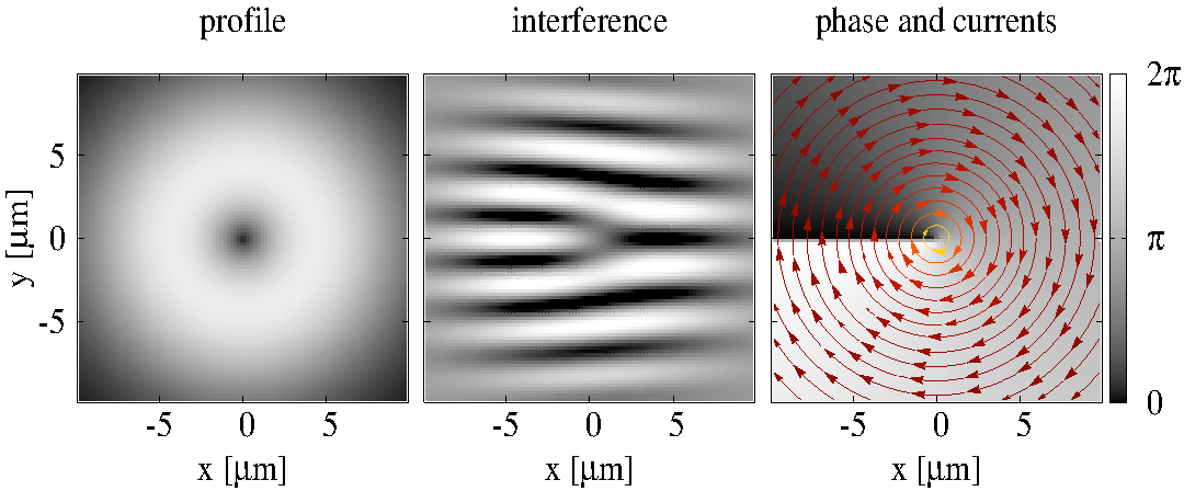
the phase of which, , linearly winds around the vortex core from to (with integer) — i.e., in cylindrical coordinates centered at the vortex core, is the azimuthal angle. This implies that the vortex carries a quantised angular momentum, . In addition, the phase has a branch-cut and therefore is not defined at the vortex core, implying the vortex wave-function has to be zero at the vortex core. An example of an vortex, with , has been plotted on the left panel of Fig. 7. Here, the phase winds clock-wise around the core, from to , and therefore the vortex current,
| (21) |
is constant at fixed distances from the vortex core, , while decreases inversely proportional to the distance (right panel of Fig. 7). Contrast this with the case of a rotational vortex in a classical fluid which rotates as a solid body with an angular velocity : Now, the fluid tangential velocity is zero at the vortex core and increases linearly with the distance, i.e., . Quantised vortices can be detected in interference fringes (middle panel of Fig. 7) as fork-like dislocations, the difference in arms giving the charge of the vortex.
3.5 Stable vortices in a small sized OPO
As explained later in Sec. 5, spontaneous stable vortices differ from metastable vortices (described in Sec. 5.1): Metastable vortices can only be injected externally, e.g. by an additional Laguerre-Gauss beam probe, into an otherwise stable symmetric state, and their persistence is due to the OPO superfluid properties [8, 22]. The metastable vortex is a possible but not unique stable configuration of the system. In contrast, as for non-resonantly pumped polaritons [80, 5], the appearance of spontaneous vortices is not a consequence of the polariton condensate being superfluid, but rather to the presence of currents related to the non-equilibrium nature of these condensates. This strongly differs from the case of equilibrium superfluids, the ground state of which is flow-less. Later, in Sec. 7 we will briefly discuss how, for polaritons non-resonantly injected into a microcavity, the presence of a confining potential can generate currents favourable to the spontaneous formation of vortices [5, 81] and vortex lattices [80].
For resonant excitation, currents arise in the OPO regime due to the simultaneous presence of pump, signal, and idler emitting at different momenta, as well as by the fact the system is finite size (see Fig. 4). We have seen in Fig. 6 that, similarly to non-resonantly pumped polaritons, the presence of a disorder potential can lead to the spontaneous appearance of vortices. However, it is remarkable that, even in the absence of disorder or trapping potentials, the OPO system can undergo spontaneous breaking of the symmetry and become unstable towards the formation of a quantised vortex state with charge if the size of the OPO is small enough [22]. This is the subject of this section. Further, as discussed in some detail later in Sec. 3.5, like for equilibrium superfluids, both stable and metastable vortices are characterised by a healing length which is determined by the parameters of the OPO system alone. Spontaneous stable vortex solutions are robust to noise (Sec. 3.5) and to any other external perturbation, and thus should be experimentally observable. However, while spontaneous vortex solutions in OPO have been observed for a toroidal pump spot 44 4 D. Sarkar (University of Sheffield), private communication., so far they have not been observed in OPO with a ‘simply connected’ pump profile, e.g., either a Gaussian or a top-hat.

Dynamical stability
As mentioned in Sec. 3.3, if the pump is shined on the -direction, , only the symmetry is left intact in the system. Clearly, this symmetry, allows for OPO solutions where the signal (and therefore also the idler) have vortex-antivortex pairs, with the vortex core position at and the antivortex core position at . However, both single and multiple vortex solutions explicitly break the symmetry and cannot be accessed by the dynamics — Note that two vortices located at opposite sides with respect to the -axis break the symmetry because of the currents.
In order to check the dynamical stability of OPO states, one has to add small fluctuations to the steady state mean-field solution: The existence of modes with positive imaginary part in the excitation spectrum indicate dynamical instability towards the growth of different modes. The dynamical stability analysis for OPO described in within the plane-wave approximation of Sec. 3.2 has been discussed in Refs. [61, 71]. Equivalently, stability can be numerically checked by introducing a weak noise. In particular, we add white noise as a quick (-like in time) pulse at a certain time to both modulus and phase of excitonic and photonic wavefunctions in momentum space, :
Both and are white noise functions, with an amplitude for the the phase , while the amplitude of the noise in the modulus is specified in units of the maximum of the pump intensity in momentum space.
Following this procedure, we have been able to single out symmetric OPO states, as shown in Fig. 8(a), which are unstable towards the spontaneous formation of stable vortex solutions. After the symmetry is broken by the noise pulse, we have observed a vortex with quantised charge () entering and stabilising into the OPO signal (idler) — Note that parametric scattering constrains the phases of pump, signal, and idler by (see Sec, 3.2), therefore an vortex in the signal at a given position implies an antivortex in the idler at the same position and vice versa. In the case of Fig. 8 and the right panel of Fig. 9, the noise strength is and ps after the noise pulse, a vortex with () enters the signal (idler) and stabilises. The strength of the noise has no relevance on the final steady state, and in particular it can be infinitesimally weak. Different noise strengths do only affect the transient time the system needs to accommodate the vortex and reach the new steady configuration. We have in addition examined whether the vortex steady state is dynamically stable by applying an additional noise pulse. For weak noise, with a strength up to , the vortex is stable and can only drift around a little before settling again into the same state. For strong noise, with strength and above, the vortex gets washed away, but after a transient period, the very same state enters and stabilises again into the signal, with the possibility of flipping vorticity 55 5 When generated by a noise pulse, both stable and metastable vortices have equal probability to have either charge . Similarly, when vortices are triggered via a Laguerre-Gauss probe, their vorticity can flip during the transient period. In particular, flipping can follow the appearance of two antivortices at the edge of the signal, one recombining with the triggered vortex. Note that the vorticity flipping conserves the total orbital angular momentum, in the sense that when for the signal flips, say, from to , for the idler the opposite happens, i.e. flips from to .. Different noise strengths do not affect the final steady state, but only the transient time.

As discussed later in Sec. 5, one can alternatively break the symmetry by a pulsed vortex probe (24), and assess whether the stable steady state is in any way dependent on the external perturbation. The homogeneous OPO states which are unstable towards the spontaneous formation of stable vortices following a white noise pulse, exhibit the same instability following a vortex Laguerre-Gauss (LG) probe pulse (see the left panel of Fig. 9). The steady state vortex is independent on both the probe intensity and size , however the weaker the probe the longer the vortex takes to stabilise, between and ps for our system parameters. As shown in Fig. 9, the stable vortex following the LG probe is exactly the same as the one triggered by a weak white noise, indicating that the probe acts only as a symmetry breaking perturbation.
Summarising, one can find OPO conditions where the symmetric solution is dynamically unstable and any symmetry breaking perturbation allows the signal and idler to relax into a stable steady state carrying a vortex with charge . For homogeneous cavities, i.e., in absence of any disorder or confining potential, we found that this requires either a small Gaussian or small top-hat like pump spot which can confine the vortex inside or a doughnut-shape pump spot. Instability of the uniform state to spontaneous pattern (e.g., vortex) formation is a typical feature of systems driven away from equilibrium [79]. Similarly we find conditions for which the uniform OPO solution is unstable to spontaneous formation of a quantised vortex. In alternative, a disorder potential breaks the symmetry explicitly and allows the pinning of stable vortex solutions in OPO, which is less surprising.
Healing length
In contrast to their classical counterpart, quantised vortices with the same angular momentum are all identical, with a size (or healing length) determined by the system non-linear properties [76]. In the case of a superfluid in equilibrium with a typical interaction energy ( is the average density) and mass , the healing length, , is the typical distance over which the condensate wave-function recovers its ‘bulk’ value around a perturbation. In particular, for an vortex (20), is the typical size of the vortex.
Similarly, in OPO, one case show that, like in equilibrium superfluids, both stable (see Sec. 3.5) and metastable (see Sec. 5) vortices are characterised by a healing length which is determined by the parameters of the OPO system alone. In particular, shape and size of the metastable vortices described in Sec. 5 are independent on the external probe. In the case of vortices in OPO, an approximate analytical expression for the vortex healing length can be derived for homogeneous pumping [22, 9], assuming that only signal and idler can carry angular momentum with opposite sign, , , while the pump remains in a plane-wave state, , as also supported by our numerical analysis. For pump powers close to OPO threshold, it can be shown [22, 9] that signal and idler steady state spatial profiles are locked together and satisfy the following complex GP equation
where . This equation describes a vortex profile [76] with a healing length given by:
| (22) |
This expression is similar to the one of an equilibrium superfluid, with the condensate density replaced by the geometric average of signal and idler densities. Further above threshold, one can show that signal and idler profiles are no longer locked together, and that they start to develop different radii. In both the simulations of Figs. 9 and 6, we find m, compatible with the estimate (22).
In Ref. [9], vortices in OPO have been created in a controlled manner by adding a weak continuous probe in resonance to the signal. Even if the phase freedom of the OPO system is explicitly broken in this configuration by the vortex cw probe, because the ratio of the probe to signal power density is low, the size of the vortex has been demonstrated to be determined by the OPO non-linear properties only rather than by the imprinting probe. In particular, a systematic study of the decrease of the vortex core radius with increasing pump power above threshold has allowed to confirm the behaviour described by the Eq. (22).
4 Triggered optical parametric oscillator regime
Before moving on into the description of metastable vortices in OPO, i.e. vortices which are transferred by a pulsed vortex probe into the OPO signal and idler, and their relation to superfluidity (Sec. 5), we describe here first the effect of an additional pulsed probe on OPO in general terms. As described previously, in the OPO regime, polaritons are continuously injected into the pump state, and undergo coherent stimulated scattering into the signal and idler states. The OPO is a steady state regime, where the filtered profiles of signal, idler, and pump, , are time independent. This also is reflected in the typical flat dispersion around pump, signal, and idler which can be observed in the OPO spectra (see Fig. 4). The group velocity of pump, signal, and idler, defined as the derivative of the energy dispersion at , is therefore zero. This however does not mean that there is no flow of polaritons, which instead is described by the phase velocity or current, (see footnote 2 on page 2), with a dominant uniform flow given approximatively by .
In resonantly pumped polaritons, in order to initiate a travelling wave-packet characterised by a finite group velocity, one needs to use an additional pulsed laser beam on top of the cw one. The description of the system is therefore still in terms of the Eqs. (9), with a total pump term given by the sum of the cw laser (10) and a probe beam :
| (23) |
For the moment being we will consider the generic case of a pulsed probe with a Gaussian space profile, shined at a momentum and energy 66 6 Note that, differently from the cw laser beam, the energy distribution spectrum of which is essentially -like, a pulsed beam has an intrinsic width in energy, proportional to the inverse pulse duration, .:
| (24) |
A pulse duration of ps (defined as the FWHM in time of ) corresponds to ps. The idea, first introduced by Ref. [20], is that the pulsed probe triggers parametric scattering 77 7 If the cw pump drives the system into the OPO regime, then the parametric scattering triggered by the pulsed probe will be in addition to the one related to OPO. However, as discussed later, the TOPO regime can be reached also in absence of the OPO. between the probe state at momentum and energy and a conjugate state at — because one can either have or , we use the state labels ‘probe’ and ‘conjugate’, rather than ‘signal’ and ‘idler’; by doing so, one also doesn’t confuse the states generated by the OPO with the additional ones generated by the probe. Both probe and conjugate states are travelling decaying states which can evolve freely from the laser probe constraints once the pulse switches off. Such states are referred to as triggered-OPO (TOPO) states. Note that a TOPO can be triggered in two regimes: either (i) in a regime where the cw laser drives the system above threshold for OPO, in which case the probe and conjugate states are the extra population states on top of the steady-state OPO signal and idler states, or (ii) when no OPO is present, i.e. for the cw pump strength below threshold. For simplicity, the numerical analysis discussed below in Sec. 4.1 is conducted in the regime (ii), but we have checked that the qualitative results also hold in the regime (i) — where, now, the steady state OPO population needs to be subtracted so that one studies the properties of the population triggered by the probe only.


4.1 Theoretical description of the TOPO
cross-refer to Fabrice Laussy’ chapter In order to analyse the dynamical evolution of a TOPO wave-packet, we study numerically the time-dependent solutions of the equations (9), with a total pump given by (23) and (24). The probe triggers parametric scattering between a probe state and a conjugate state. In the majority of cases, as discussed in Ref. [23], the parametric scattering is too weak to induce any significant amplification, and an exponential decay of both probe and conjugate populations is observed immediately after the probe switches off. Here, the spectrum shows a strong emission from the pump state and a weak emission from the LP states mainly at momenta and .
However, we have found conditions under which both signal and conjugate states get initially strongly amplified by the parametric scattering from the pump, then decay slowly and, only at later times, decay exponentially (see Figs. 10 and 11) --- we refer to this as the ‘proper’ TOPO regime. A similar behaviour has been also observed in experiments 88 8 See, for example, Fig. 3 of Ref. [82], where the intensity maximum of the extra population is reached within ps after the maximum of the pulsed probe, is followed by a slow decay. . Now, the spectrum is observed to be linear, (see Fig. 10). A linear spectrum can be explained by the fact that, in order to have efficient parametric scattering, probe and conjugate state must have a large spatial overlap and therefore similar group velocities. Thus signal and conjugate group velocities need to lock, which is only possible if the dispersion becomes linear — a similar result has been also found in 1D simulations (see Fabrice Laussy’s Chapter), as well as in experiments [20]. The group velocity is defined as the derivative of the energy dispersion with respect to the momentum. However, we can also measure it from the probe and the conjugate density variations in time, i.e., as , where is the maximum of either the probe or conjugate spatial profile, which we use as a reference. By analysing the change in time of the spatial profile of the TOPO probe state , it is possible to show [23] that its group velocity is given exactly by the derivative of the lower polariton (LP) dispersion evaluated at , i.e., for zero detuning and low densities by (see Fig. 12). This behaviour is consistent with the form of the spectrum shown in Fig. 10 99 9 In the regime where the probe generates only a weak parametric scattering, aside the strong emission from the pump state, the dispersion is simply that of the LP, and thus is not surprising that the signal propagates with a group velocity given by . Remember that here the cw pump is below threshold for OPO.. Further, we have been able to determine [23] that the TOPO linear dispersion is tangential to the LP branch at , thus its slope is given in this case also by .

From the PL spectrum we can also deduce the nature of the wave-packet propagation. For systems characterised by a linear dispersion, like in the TOPO regime, one expects a soliton-like behaviour, where probe and conjugate states propagate without changing neither their shape nor intensity. For quadratic dispersion, a Gaussian wave-packet moves at a constant velocity and it preserves its overall shape in time but its width grows (FWHM=) [76]. Note, however, that, due to the finite polariton lifetime, the total density decays exponentially, with a rate given by at zero detuning. Finally, for non-quadratic dispersion, propagation becomes complex: The wave-packet gets distorted and there are beatings in the spatial profiles. In general, due to the dynamical nature of the TOPO state, the system evolves between these different scenarios. In particular, only in the strong amplification regime the spectrum is linear, while it evolves back to the LP one at longer times. However, for a one-dimensional version of the equations (9), and for uniform, infinitely extended in space, pumping spots, non-decaying, soliton solutions have been recently found [83]. This has been also generalised to a two-dimensional infinite systems [84], where, for some narrow range of pumping strengths, a soliton-like behaviour has been predicted for and . However, to date, a non-decaying wave-packet propagation has not been found in experiments.
Finally we would like to note that, the typical behaviour of probe and conjugate states (left panel of Fig. 12) is analogous to the one discussed in four-wave-mixing experiments [85, 86]: when the probe arrives, and shortly after that, the conjugate propagates faster then the probe, before getting locked to it with a small spatial shift of their maximum intensities. At later times, when the density drops and the parametric process becomes inefficient, the two wave-packets start unlocking — the conjugate slows down with respect to the signal if as in Fig. 12, or it moves faster when .
4.2 Experiments
The TOPO regime has been recently studied in experiments in Refs. [20, 45] (for a review see Ref. [87]). As previously described, the additional pulsed probe has been used to create a travelling, long-living, coherent polaritons signal, continuously fed by the OPO. A large increase of the signal lifetime has been observed for a pump intensity approaching and exceeding the OPO threshold [45]. This observation can be explained in terms of a critical slowing down of the dynamics following appearance of a soft Goldstone mode in the spectrum close to threshold. It is also consistent with the nature of wave-packet propagation in systems with linear dispersion. This has been used to interpret subsequent experiments, where the linearisation of dispersion leads to the suppression of weak scattering and therefore to a polariton motion without any dissipation [20, 87] cross refer to Fabrice Laussy’ chapter. Due to the finite size of the excitation spot, the travelling TOPO signal lives only as long as it reaches the edge of the excitation spot. However, as discussed in detail in Ref. [87], in order to asses the sustainability in time of the TOPO process, both pump and probe beams can be chosen so that the probe state forms at . In such a case, the polaritons in the probe state are not travelling and therefore and it is thus possible to measure the lifetime of the TOPO wave-packet, which is of the order of a nanosecond. The decay of the TOPO population in time, as well as the finite lifetime of TOPO pulses, indicate that the soliton behaviour predicted in Ref. [84] is not the explanation of the current experiments. However, the linearisation of the system’s dispersion due to the parametric process, as well as the appearance of the Goldstone mode, provide a sufficient explanation of dissipationless propagation in free space, as well as frictionless flow against an obstacle, during the part of the dynamics when parametric processes are strong and the spectrum linear.
5 Triggered metastable vortices as a diagnostic of the OPO superfluid properties
OPO condensates, as well as polariton condensates pumped incoherently, share with weakly interacting Bose-Einstein condensates at equilibrium phenomena like the spontaneous breaking of the phase symmetry and the appearance of a Goldstone mode (see Sec. 3.2). However, being intrinsically non-equilibrium, all polaritonic systems need continuous pumping to balance the fast decay and maintain a steady state regime. In strong contrast with equilibrium superfluids, the ground state of which is flow-less, pump and decay lead to currents that carry polaritons from gain to loss dominated regions. This can lead to the spontaneous formation of vortices: The presence of currents in polariton condensates can lead to the spontaneous appearance of vortices without invoking any superfluid properties. This is true for incoherently pumped polaritons in presence of a confining potential [5, 80, 81], as well as for polaritons in the OPO regime, with the difference that here, even in the absence of disorder or a trapping potential, the system becomes unstable towards the formation of a quantised vortex state with charge (see Sec. 3.5). In addition, the hydrodynamic nucleation of quantised vortices can appear as a consequence of the collisions of a moving polariton fluid with an obstacle, as will be briefly discussed in Sec. 7. Therefore, in general, for polaritonic systems, one has to apply some care when using the appearance of vortices as a diagnostic for the superfluid properties of such a non-equilibrium system.
In the case of equilibrium superfluids, the rotation of a condensate is accompanied, above a critical angular velocity [76, 75], by the creation of quantised vortices. Here, vortices are stable as far as the system is kept rotating and become unstable when the imposed rotation is halted [77]. However, persistent flow can be observed when a BEC is confined into a toroidal trap and the quantised rotation is initiated by a pulsed Laguerre-Gauss beam [88, 89, 90]. The toroidal trap is essential to allow the vortex stability, because of the energy cost of the vortex core to move through the high density region from the center of the torus where the density is zero. The very same idea of questioning the persistency of flow in a BEC via a pulsed Laguerre-Gauss beam as a diagnostic for superfluidity, can be applied to polaritons 1010 10 Note, however, that even if in the atomic and polaritonic case the same Laguerre-Gauss laser field is used, the mechanism of spinning the BEC atoms is different from the one which rotates polaritons.. As recently proposed for non-resonantly pumped polariton condensates in Ref. [21], this definition of superfluidity as metastable flow is equally meaningful in non-equilibrium systems as in equilibrium ones. However, as we will see, the important difference is that, in the OPO regime, flow persistency is possible even in a simply connected geometry, i.e., without the need of a toroidal trap which pins the vortex.
A pulsed Laguerre-Gauss (LG) probe beam carrying a vortex of charge can be described by:
| (25) |
with can be tuned resonantly to either the OPO signal or idler. As discussed in the next section, by using a pulsed LG beam (25), vorticity has been shown to persist not only in absence of the rotating drive, but also longer than the gain induced by the probe, and therefore to be transferred to the OPO signal, demonstrating metastability of quantised vortices and persistence of currents in OPO. Experiments and theory will be discussed in the next Sec. 5.1.

5.1 Theory and experiments
In the case of metastable vortex solutions, the symmetric vortex-less OPO steady state is dynamically stable, but, because of its superfluid properties, can support persistent metastable currents injected externally. From a theoretical point of view, metastable solutions can be equally induced by either a vortex probe pulse (25) or a noise pulse. However, differently from the case of stable vortices, metastable solutions require a threshold in the perturbation breaking the system symmetry. For the simulations of Ref. [8], as we were interested mainly into the transfer of angular momentum from the probe into the OPO signal and idler, we have been considering conditions where the parametric scattering induced by the probe is too weak to induce any significant long-lasting amplification, and the gain introduced by the probe on top of the OPO disappears quite quickly. We have found conditions where the vortex is transferred from the probe into the signal 1111 11 We checked that () vortex solutions can appear only into the OPO signal (idler). A vortex probe pulse of any charge injected resonantly to the pump momentum and energy gets immediately transferred to an () vortex in the signal (idler), leaving the pump vortex-less. (and antivortex in the idler) immediately 1212 12 Later, in Sec. 6.1, in connection to the stability of multiply quantise vortices, we also describe vortices in the TOPO regime, where we follow the vortex dynamics not of the OPO like here, but of the extra population only. when the probe is shined. The transfer is followed by a transient time during which the imprinted vortex drifts around inside the signal and in certain cases settles into a metastable solution. Similarly to what happens to stable vortex solutions, we have found that the spatial position of the metastable steady state vortices is close to the position where the OPO signal has the currents pointing inwards (see second panel of Fig. 5). The influence of currents on the formation of vortices is discussed further in Sec. 5.2. Such metastable solutions do not always exist: if the probe is positioned well inside a wide OPO signal, as the creation of a vortex is accompanied by the creation of an antivortex (see Sec. 5.2), often, the vortex-antivortex pair quickly recombines; in other cases, during the transient period, the excited vortex can spiral out of the signal. Finally note that, as discussed in Sec. 3.5, the shape and the size of metastable vortices are independent on the external probe but are only determined by the parameters of the OPO.
In the experiment of Ref. [8] also shown in Fig. 13, a vortex is excited by a probe smaller than that of the signal to allow free motion of the vortex within the condensate. Vortices are detected, and their evolution in time followed by a streak camera, in interference images, generated by making interfere the OPO signal with a constant phase reference beam in a Michelson interferometer (second row of Fig. 13). As single shot measurements would give a too low signal to noise ratio, every picture is the result of an average over many pulsed experiments taken always for the same OPO conditions. The probe triggers a TOPO response, creating a strong gain and an extra decaying population on top of the OPO signal (TOPO). In experiments, different regimes have been investigated. In particular, it has been possible to establish that, only under very high pump power and at specific points in the sample, the vorticity was transferred from the TOPO into the OPO signal, generating a metastable vortex solution. This not only demonstrates that the OPO polariton condensate can show unperturbed rotation, but also that a vortex can be another metastable solution of the final steady state, demonstrating therefore the superfluid behaviour in the non-equilibrium polariton OPO system. After the vortex is imprinted into the OPO signal, it has been possible to observe the vortex core slowly drifting, changing in shape and moving with different velocities. Note that, because these are metastable solutions, a minimum probe power is required for the polaritons to acquire enough angular momentum to be able to transfer it to the steady state. However, once the transfer is achieved, the probe power does not change significantly the duration and depth of the vortex in the steady state.
5.2 Onset and dynamics of vortex-antivortex pairs
There is an aspect that we have been neglecting in the discussion of the previous section on the occurrence of metastable vortex solutions in OPO triggered by an external LG probe. If the extension of the probe carrying a vortex with charge is smaller than the size of the vortex-free OPO signal, continuity of the polariton wavefunction requires that necessarily an antivortex with charge has to form at the edge of the probe (see Fig. 14). Indeed, ‘unintended’ antivortices have been shown to appear in the signal at the edge of the imprinting vortex probe and we have explained in Ref. [91], both theoretically and via experiments, the origin of the deterministic behaviour of the antivortex onset and dynamics, i.e. where antivortices are more likely to appear in terms of the currents of the imprinting probe and the ones of the underlying OPO.

Random phase between pump and probe
As mentioned earlier in Sec. 5.1, single shot measurements would give a too low signal to noise ratio, therefore an average is performed over many pulsed experiments taken always for the same OPO conditions. What differs at each probe arrival is the random relative phase between pump and probe,
| (26) |
with uniformly distributed between and . We simulate the dynamics of the vortex-free signal OPO (same conditions of Fig. 6 at ) following the arrival of a vortex probe (24) for 1000 realisations of and then average the complex wavefunctions over such realisations at fixed time and space, .
The steady state currents of the OPO signal before the arrival of the probe have a dominant component pointing leftwards and an equilibrium position where all currents point inwards (bottom left part of the panel (a) in Fig. 14). In single shot simulations of Fig. 14(d,f) (one realisation of the phase ), we find that if the probe is positioned well inside the OPO signal, then the imprinting of a vortex (antivortex ) forces the system to generate, at the same time, an antivortex (vortex ) at the edge of the probe. This is a consequence of the continuity of the polariton wavefunctions: If the signal OPO phase is homogeneous and vortex-free before the arrival of the probe, then imposing a topological defect, i.e., a branch cut, on the signal phase at the probe core, requires the branch cut to terminate where the phase is not imposed by the probe any longer and has to continuously connect to the freely chosen OPO signal phase, i.e. at the edge of the probe. As repeatedly mentioned in this review, OPO parametric scattering processes constrain the sum of signal and idler phases to the phase of the laser pump by . Thus, at the same positions where the V-AV pair appears in the signal, an AV-V pair appears in the idler, so that locally the phase constraint described above is satisfied. This agrees with the experiments in [9], though there only a single V (AV) in the signal (idler) could be detected, because the signal size was comparable to the probe one.
Different relative phases cause the antivortex (vortex) to appear in different locations around the vortex (antivortex) probe. However, on 1000 realisations of the random phase uniformly distributed between and , we observe that the antivortices (vortices) are more likely to appear on positions where the current of the steady state OPO signal before the probe arrival and the probe current are opposite. For example, for the () probe of Fig. 14(c) (Fig. 14(e)), the current constantly winds anti-clockwise (clockwise), therefore, comparing with the signal current of Fig. 14(a), the two are anti-parallel in the bottom right (top left) region on the probe edge, region where is very likely that an antivortex (vortex) is formed. Note also that the onset of antivortices (vortices) privileges regions where the steady OPO signal has a minimal intensity. This agrees remarkably well with it has been recently measured experimentally, in Ref. [91].
Multi-shot averaged dynamics
Crucially, via numerical simulations, we elucidate the reason why an experimental average over many shots allows detecting a vortex by direct visualisation in density and phase profiles. Recently, it has been suggested by stochastic simulations [21] that vortices in non-resonantly pumped polariton condensates undergo a random motion which will hinder their direct detection, unless they are close to be pinned by the stationary disorder potential and thus follow a deterministic trajectory [7]. In the case considered here of a superfluid generated by OPO, we can instead explain a deterministic dynamics of the V-AV pair in terms of the OPO steady state currents, which determine a unique trajectory for the pair, allowing their observation in multi-shot measurements.
By averaging the 1000 images obtained at the probe arrival, e.g., in Fig. 14(c), neither the imprinted vortex nor the antivortex can be detected: Both phase singularities are washed away by averaging the differently positioned branch-cuts. However, the steady state signal currents push the V and AV, initially positioned in different locations, towards the same equilibrium position where all currents point inwards. Thus, exactly at the time where the probe is shined, on average there is no V-AV pair, after ps, both V and AV appear and last ps (see Ref. [91]), till they eventually annihilate.
It is interesting to note that it has been experimentally shown [91] that the onset of vortices in polariton superfluids does not require a LG imprinting beam, but instead vortex-antivortex pairs can be also generated when counter-propagating currents are imposed, similarly to what happens in normal (classical) fluids. In Ref. [91] a Gaussian pulsed beam has been shined either at rest with respect to the OPO signal, , or moving . While no vortex-antivortex pair appears in the first case, in the second, a vortex-antivortex pair appears on opposite sides of the probe edge.
6 Stability of multiply quantised vortices
The energy of a vortex is proportional to its quantum of circulation squared [76], . Thus, ignoring interactions, a doubly charged vortex, has higher energy than two single vortices. However, including interactions between vortices, the energy of an vortex turns to be the same as the energy of two interacting vortices close together. The behaviour of doubly quantised vortices has been the subject of intensive research in the context of ultra-cold atomic gases. In particular, it has been established that the nature of the splitting is the dynamical instability. Nevertheless, vortices have been predicted to be stable for specific ranges of density and interaction strength [92, 93], though, so far, they have not been observed experimentally [94]. As for single vortices, multiply quantised vortices can be however stabilised in multiply connected geometry. Indeed, stable pinned persistent vortices have been recently observed [89] by using a toroidal pinning potential generated by an external optical plug, and demonstrated to split soon after the plug was removed. In this case, the presence of a plug beam at the vortex center can pin both and vortex states and stabilise them against respectively spiralling out of the condensate for and splitting for . In other words, the external trap mechanically prevents the persistent flow to undergo any movement.
In contrast to equilibrium superfluids, such as atomic gases, both stable and unstable vortices has been experimentally realised in polariton OPO superfluids [8]. In this section we provide a theoretical explaination of the stability and splitting of doubly charged polariton vortices. As done previously, vortices in OPO are generated by an external pulsed probe (25). As such, we classify the response of the system to an LG probe, depending whether the probe generates a TOPO state (and the vortex is only carried by the extra population but is not transferred into the OPO signal), as described in Sec. 6.1, or instead is transferred in the OPO signal (Sec. 6.2).
6.1 TOPO regime
We first consider the TOPO regime (see Sec. 4), i.e., when the vortex propagates inside the triggered probe and conjugate wave-packets. It has been found [8, 23] that, in the TOPO regime, vortices are stable within their lifetime when triggered at small momenta (see Fig. 15 panels (a) and (b)), while they split into two vortices for large values of (see Fig. 15 panels (c) and (d)). This conclusion was reached both by experimental observations [8] and theoretical analysis [8, 23]. The numerical analysis shows that the crossover from non-splitting to splitting happens for the probe momenta where the LP dispersion deviates from the quadratic one (see Fig. 12). The two different cases are shown in Fig. 15: For = 0.2m-1, at short times, the probe propagates without changing shape and with little change in intensity (not shown in the Fig. 15), consistent with the linear dispersion of spectrum characterising this regime. However, at longer times the density of the triggered probe and conjugate states drops more then two orders of magnitude, the dispersion changes to the quadratic one and the wave-packet expands (panel (b)). A uniform expansion of the wave-packet leads to the decrease of the probe and the conjugate polariton densities and thus to an increase of the vortex core, but it does not cause the vortex to split. In contrast, for = 1.4m-1, where the LP dispersion is not quadratic, the vortex state splits into two vortices shortly after the arrival of the probe (panel (d)). This behaviour can be understood by analysing the evolution of the system’s excitation spectrum in time: the dispersion of the time-dependent TOPO evolves from LP (before the probe arrival) to linear (at early times after the probe arrival, when the stimulated scattering is strong), and back to the LP at later times. For large the LP dispersion deviates strongly from quadratic (see Fig. 12 right panel). Wave-packets propagating with non-quadratic dispersion do not keep their shapes (as discussed in Sec. 4.1), and the simulations show that the distortion can be very pronounced in particular at later times of the evolution. The distortion during the early times of the propagation leads to the mechanical splitting of an vortex, analogous to the structural instability discussed in Ref. [95]. Additionally, as discussed in Ref. [8], for small , within the quadratic part of the dispersion, the group velocity of the wave-packet carrying the vortex equals the velocity of the net super-current (given by ) associated with phase variations. This is not however the case for larger , beyond the quadratic part of the dispersion. In this case, the propagating vortex feels a net current in its moving reference frame, which may provide additional mechanism for splitting.

6.2 OPO regime
In contrast to the TOPO regime described above, it has been shown both experimentally and theoretically [8, 23] that vortices that do get imprinted into the steady-state OPO signal are never stable and splits into two vortices almost immediately, even before the probe reaches its maximum intensity (see Fig. 16). By analysing the system’s dispersion in different regimes, as well as the dynamics of currents visible in the simulations, we have been able to identify several causes for the splitting: Before the arrival of the probe, the steady-state OPO dispersion is flat around the pump, signal, and idler. However, the triggering probe favours the signal and conjugate to lock and propagate with the same velocity . This behaviour corresponds to a linear dispersion. Further, once the vortex gets imprinted into the stationary OPO signal and idler, the system’s dispersion changes back to be flat. The evolution of the dispersion between flat, linear and again flat leads to a complicated dynamics of both signal and idler (the transient period described in [22]), causing the structural instability and splitting of the vortex during the transient time. Another reason for the structural instability and splitting are the non-uniform currents (see Fig. 16) present in the OPO signal caused by the interplay between spatial inhomogeneity, pump and decay, which the OPO vortex experiences in its reference frame.

7 Vortices in other polariton fluids
We do not pretend to give an exhaustive review of the broad field which studies vortices in polariton fluids in this chapter, where we have mostly focussed on the occurrence of vortices in polariton OPO superfluids. However, we would like at least to briefly mention what happens for polariton fluids other than OPO.
Spontaneous vortices in trapped incoherently pumped polaritons
For incoherently pumped polaritons, the presence of a harmonic trapping potential, can make the non-rotating solution unstable to the spontaneous formation of a vortex lattice [80] (this work has been generalised to include the effects of polarisation in Ref. [96]). In experiments, spontaneous vortices in incoherently pumped systems, have been observed in Refs. [5, 97] and their existence explained in terms of pinning by the disorder present in the CdTe sample. Adding the polarisation degrees of freedom, can give rise to the appearance of half-vortices [98, 6]. Polariton vortices have been also observed in cavity mesas [81]. cross refer to Benoit Deveaud’s chapter?
Vortex-antivortex pairs have been observed in the non-resonantly pumped experiments of Ref. [10], where the mechanism of V-AV generation is explained in terms of density fluctuations originating from the cw multi-mode pumping laser, while for a single-mode laser no V-AV pairs have been observed. In this sense, their motivation and interpretation is in terms of the BKT transition. The pair dynamics in the condensate has been studied in Ref. [99]. cross refer to Yoshisha Yamamoto’s chapter?
Finally, as mentioned previously in Secs.5 and 5.2, generation and detection of metastable vortices have been also recently discussed for polariton condensates generated by toroidal non-resonantly pumping in Ref. [21], where vortices have been seeded with an external LG probe. Interestingly, very recently in Ref. [100], it has been observed an all-optical spontaneous pattern formation in a polariton condensate non-resonantly pumped with a ring geometry.
Resonantly pumped-only polaritons
In Ref. [11, 12], the hydrodynamic nucleation of V-AV pairs is studied by making collide the polariton fluid with a large defect. In particular, polaritons are resonantly (coherently) injected with a pulsed laser beam, creating a population in the pump state only. The focus and interest of these studies are the possibility of exploring quantum turbulence, the appearance of dissipation and drag above a critical velocity because of the nucleation of vortices in the wake of the obstacle.
Acknowledgements.
We would like to acknowledge fruitful collaborations with A. Berceanu, E. Cancellieri, D. Sanvitto, C. Tejedor, and D. M. Whittaker on some of the topics discussed in this review, as well as the collaboration with the experimental group at UAM in Madrid (C. Antón, M. Baudisch, G. Tosi, L. Viña). We are particularly grateful to I. Carusotto and J. Keeling for stimulating discussions and for the critical reading of this manuscript. We also would like to thank C. Creatore, B. Deveaud-Plédran, and Y. Yamamoto for useful suggestions and points of discussion. F.M.M. acknowledges the financial support from the programs Ramón y Cajal and POLATOM (ESF). This work has been also supported by the Spanish MEC (MAT2008-01555, QOIT-CSD2006-00019), CAM (S-2009/ESP-1503) and FP7 ITN ”Clermont4” (235114).References
- (1) L. Onsager, Nuovo Cimento 6, 249 (1949)
- (2) R. Feynman, Application of Quantum Mechanics to Liquid Helium, Progress in Low Temperature Physics, vol. 1 (Elsevier, 1955)
- (3) J.F. Nye, M.V. Berry, Proc. R. Soc. A 336, 165 (1974)
- (4) K. Staliunas, V.J. Sanchez-Morcillo, Transverse Patterns in Nonlinear Optical Resonators (Springer-Verlag, Berlin, 2003)
- (5) K.G. Lagoudakis, M. Wouters, M. Richard, A. Baas, I. Carusotto, R. André, L.S. Dang, B. Deveaud-Plédran, Nature Physics 4, 706 (2008)
- (6) K.G. Lagoudakis, T. Ostatnický, A.V. Kavokin, Y.G. Rubo, R. André, B. Deveaud-Plédran, Science 326, 974 (2009)
- (7) K.G. Lagoudakis, F. Manni, B. Pietka, M. Wouters, T.C.H. Liew, V. Savona, A.V. Kavokin, R. André, B. Deveaud-Plédran, Phys. Rev. Lett. 106, 115301 (2011)
- (8) D. Sanvitto, F. Marchetti, M. Szymańska, G. Tosi, M. Baudisch, F. Laussy, D. Krizhanovskii, M. Skolnick, L. Marrucci, A. Lemaître, J. Bloch, C. Tejedor, L.V. na, Nature Physics 6, 527 (2010)
- (9) D.N. Krizhanovskii, D.M. Whittaker, R.A. Bradley, K. Guda, D. Sarkar, D. Sanvitto, L. Viña, E. Cerda, P. Santos, K. Biermann, R. Hey, M.S. Skolnick, Phys. Rev. Lett. 104, 126402 (2010)
- (10) G. Roumpos, M.D. Fraser, A. Löffler, S. Höfling, A. Forchel, Y. Yamamoto, Nature Physics 7, 129 (2011)
- (11) G. Nardin, G. Grosso, Y. Leger, B. Pietka, F. Morier-Genoud, B. Deveaud-Plédran, Nature Physics (2011). DOI doi:10.1038/nphys1959
- (12) D. Sanvitto, S. Pigeon, A. Amo, D. Ballarini, M.D. Giorgi, I. Carusotto, R. Hivet, F. Pisanello, V.G. Sala, P.S. Soares-Guimaraes, R. Houdre, E. Giacobino, C. Ciuti, A. Bramati, G. Gigli, arXiv:1103.4885 (2011)
- (13) J. Kasprzak, M. Richard, S. Kundermann, A. Baas, P. Jeanbrun, J.M.J. Keeling, F.M. Marchetti, M.H. Szymańska, R. André, J.L. Staehli, V. Savona, P.B. Littlewood, B. Devaud, L.S. Dang, Nature 443 (2006)
- (14) H. Deng, H. Haug, Y. Yamamoto, Rev. Mod. Phys. 82, 1489 (2010)
- (15) I. Carusotto, presented at ICSCE4, Cambridge, UK (available at http://tcm.phy.cam.ac.uk/BIG/icsce4/talks/carusotto.pdf) (2008)
- (16) J. Keeling, N.G. Berloff, Nature 457, 273 (2009)
- (17) J. Keeling, N. Berloff, Contemporary Physics 52, 131 (2011)
- (18) R.M. Stevenson, V.N. Astratov, M.S. Skolnick, D.M. Whittaker, M. Emam-Ismail, A.I. Tartakovskii, P.G. Savvidis, J.J. Baumberg, J.S. Roberts, Phys. Rev. Lett. 85, 3680 (2000)
- (19) J.J. Baumberg, P.G. Savvidis, R.M. Stevenson, A.I. Tartakovskii, M.S. Skolnick, D.M. Whittaker, J.S. Roberts, Phys. Rev. B 62, R16247 (2000)
- (20) A. Amo, D. Sanvitto, F.P. Laussy, D. Ballarini, E. del Valle, M.D. Martin, A. Lemaitre, J. Bloch, D.N. Krizhanovskii, M.S. Skolnick, C. Tejedor, L.V. na, Nature 457, 291 (2009)
- (21) M. Wouters, V. Savona, Phys. Rev. B 81, 054508 (2010)
- (22) F.M. Marchetti, M.H. Szymańska, C. Tejedor, D.M. Whittaker, Phys. Rev. Lett. 105, 063902 (2010)
- (23) M.H. Szymańska, F.M. Marchetti, D. Sanvitto, Phys. Rev. Lett. 105, 236402 (2010)
- (24) A.V. Gorbach, R. Hartley, D.V. Skryabin, Phys. Rev. Lett. 104, 213903 (2010)
- (25) M.S. Skolnick, T.A. Fisher, W.D. M., Semicond. Sci. Technol. 13, 645 (1998)
- (26) V. Savona, C. Piermarocchi, A. Quattropani, P. Schwendimann, F. Tassone, Phase Transitions 68, 169 (1999)
- (27) G. Khitrova, H.M. Gibbs, F. Jahnke, M. Kira, S.W. Koch, Rev. Mod. Phys. 71, 1591 (1999)
- (28) C. Ciuti, P. Schwendimann, A. Quattropani, Semicond. Sci. Technol. 18, S279 (2003)
- (29) J. Keeling, F.M. Marchetti, M.H. Szymańska, P.B. Littlewood, Semicond. Sci. Technol. 22, R1 (2006)
- (30) Y. Yamamoto, A. İmamoğlu, Mesoscopic Quantum Optics (Wiley, New York, 1999)
- (31) Y. Yamamoto, F. Tassone, H. Cao, Semiconductor Cavity Quantum Electrodynamics, Springer Tracts in Modern Physics, vol. 167 (Springer-Verlag, Berlin, 2000)
- (32) A. Kavokin, G. Malpuech, Cavity Polaritons, Thin Films and Nanostructures, vol. 32 (Elsevier, NY, 2003)
- (33) A.V. Kavokin, J.J. Baumberg, G. Malpuech, F.P. Laussy, Microcavities (Oxford University Press, Oxford, 2007)
- (34) C. Ciuti, V. Savona, C. Piermarocchi, A. Quattropani, P. Schwendimann, Phys. Rev. B 58, 7926 (1998)
- (35) G. Rochat, C. Ciuti, V. Savona, C. Permarocchi, A. Quattropani, P. Schwendimann, Phys. Rev. B 61, 13856 (2000)
- (36) R. Houdré, C. Weisbuch, R.P. Stanley, U. Oesterle, M. Ilegems, Phys. Rev. Lett. 85, 2793 (2000)
- (37) A.I. Tartakovskii, D.N. Krizhanovskii, D.A. Kurysh, V.D. Kulakovskii, M.S. Skolnick, J.S. Roberts, Phys. Rev. B 65, 081308 (2002)
- (38) D.N. Krizhanovskii, A.I. Tartakovskii, V.D. Kulakovskii, M.S. Skolnick, J.S. Roberts, Phys. Rev. B 66, 165329 (2002)
- (39) R. Butté, M.S. Skolnick, D.M. Whittaker, D. Bajoni, J.S. Roberts, Phys. Rev. B 68, 115325 (2003)
- (40) N.A. Gippius, S.G. Tikhodeev, V.D. Kulakovskii, D.N. Krizhanovskii, A.I. Tartakovskii, EPL (Europhysics Letters) 67, 997 (2004)
- (41) A. Baas, J.P. Karr, M. Romanelli, A. Bramati, E. Giacobino, Phys. Rev. Lett. 96, 176401 (2006)
- (42) D. Sanvitto, D.N. Krizhanovskii, D.M. Whittaker, S. Ceccarelli, M.S. Skolnick, J.S. Roberts, Phys. Rev. B 73, 241308 (2006)
- (43) D.N. Krizhanovskii, D. Sanvitto, A.P.D. Love, M.S. Skolnick, D.M. Whittaker, J.S. Roberts, Phys. Rev. Lett. 97, 097402 (2006)
- (44) D.N. Krizhanovskii, S.S. Gavrilov, A.P.D. Love, D. Sanvitto, N.A. Gippius, S.G. Tikhodeev, V.D. Kulakovskii, D.M. Whittaker, M.S. Skolnick, J.S. Roberts, Phys. Rev. B 77, 115336 (2008)
- (45) D. Ballarini, D. Sanvitto, A. Amo, L. Viña, M. Wouters, I. Carusotto, A. Lemaitre, J. Bloch, Phys. Rev. Lett. 102, 056402 (2009)
- (46) M.S. Skolnick, D.M. Whittaker, R. Butté, A.I. Tartakovskii, Semiconductor Science and Technology 18, S301 (2003)
- (47) C. Ciuti, P. Schwendimann, A. Quattropani, Phys. Rev. B 63, 041303 (2001)
- (48) W. Langbein, Phys. Rev. B 70, 205301 (2004)
- (49) P.G. Savvidis, J.J. Baumberg, R.M. Stevenson, M.S. Skolnick, D.M. Whittaker, J.S. Roberts, Phys. Rev. Lett. 84, 1547 (2000)
- (50) P.G. Savvidis, J.J. Baumberg, R.M. Stevenson, M.S. Skolnick, D.M. Whittaker, J.S. Roberts, Phys. Rev. B 62, R13278 (2000)
- (51) R. Huang, F. Tassone, Y. Yamamoto, Phys. Rev. B 61, R7854 (2000)
- (52) G. Dasbach, T. Baars, M. Bayer, A. Larionov, A. Forchel, Phys. Rev. B 62, 13076 (2000)
- (53) J. Erland, V. Mizeikis, W. Langbein, J. Jensen, N. Mortensen, J. Hvam, physica status solidi (b) 221, 115 (2000)
- (54) G. Messin, J.P. Karr, A. Baas, G. Khitrova, R. Houdré, R.P. Stanley, U. Oesterle, E. Giacobino, Phys. Rev. Lett. 87, 127403 (2001)
- (55) M. Saba, C. Ciuti, J. Bloch, V. Thierry-Mieg, R. André, L.S. Dang, S. Kundermann, A. Mura, G. Bongiovanni, J.L. Staehli, B. Deveaud, Nature 414, 731 (2001)
- (56) P.G. Savvidis, C. Ciuti, J.J. Baumberg, D.M. Whittaker, M.S. Skolnick, J.S. Roberts, Phys. Rev. B 64, 075311 (2001)
- (57) S. Kundermann, M. Saba, C. Ciuti, T. Guillet, U. Oesterle, J.L. Staehli, B. Deveaud, Phys. Rev. Lett. 91, 107402 (2003)
- (58) A. Huynh, J. Tignon, O. Larsson, P. Roussignol, C. Delalande, R. André, R. Romestain, L.S. Dang, Phys. Rev. Lett. 90, 106401 (2003)
- (59) C. Diederichs, J. Tignon, G. Dasbach, C. Ciuti, A. Lamaitre, J. Bloch, P. Roussignol, C. Delalande, Nature 440, 904 (2006)
- (60) G.K. Campbell, J. Mun, M. Boyd, E.W. Streed, W. Ketterle, D.E. Pritchard, Phys. Rev. Lett. 96, 020406 (2006)
- (61) D.M. Whittaker, Phys. Rev. B 71, 115301 (2005)
- (62) C. Ciuti, I. Carusotto, Physica Status Solidi B 242, 2224 (2005)
- (63) M. Wouters, I. Carusotto, Phys. Rev. B 75, 075332 (2007)
- (64) A. Baas, J.P. Karr, M. Romanelli, A. Bramati, E. Giacobino, Phys. Rev. B 70, 161307 (2004)
- (65) L. Cavigli, M. Gurioli, Phys. Rev. B 71, 035317 (2005)
- (66) N.A. Gippius, I.A. Shelykh, D.D. Solnyshkov, S.S. Gavrilov, Y.G. Rubo, A.V. Kavokin, S.G. Tikhodeev, G. Malpuech, Phys. Rev. Lett. 98, 236401 (2007)
- (67) C. Adrados, A. Amo, T.C.H. Liew, R. Hivet, R. Houdré, E. Giacobino, A.V. Kavokin, A. Bramati, Phys. Rev. Lett. 105, 216403 (2010)
- (68) T.K. Paraïso, M. Wouters, Y. Léger, F. Morier-Genoud, B. Deveaud-Plédran, Nature Materials 9, 655 (2010)
- (69) E. Cancellieri, F.M. Marchetti, M.H. Szymańska, C. Tejedor, Phys. Rev. B 83, 214507 (2011)
- (70) A. Amo, S. Pigeon, C. Adrados, R. Houdré, E. Giacobino, C. Ciuti, A. Bramati, Phys. Rev. B 82, 081301 (2010)
- (71) M. Wouters, I. Carusotto, Phys. Rev. A 76, 043807 (2007)
- (72) I. Carusotto, C. Ciuti, Phys. Rev. B 72, 125335 (2005)
- (73) M.H. Szymańska, J. Keeling, P.B. Littlewood, Phys. Rev. Lett. 96, 230602 (2006)
- (74) M. Wouters, I. Carusotto, Phys. Rev. Lett. 99, 140402 (2007)
- (75) G.B. Hess, W.M. Fairbank, Phys. Rev. Lett. 19, 216 (1967)
- (76) L.P. Pitaevskii, S. Stringari, Bose-Einstein Condensation (Clarendon Press, Oxford, 2003)
- (77) D.S. Rokhsar, Phys. Rev. Lett. 79, 2164 (1997)
- (78) D.M. Whittaker, phys. stat. sol. (c) 2, 733 (2005)
- (79) M.C. Cross, P.C. Hohenberg, Rev. Mod. Phys. 65, 851 (1993)
- (80) J. Keeling, N.G. Berloff, Phys. Rev. Lett. 100, 250401 (2008)
- (81) G. Nardin, K.G. Lagoudakis, B. Pietka, F.m.c. Morier-Genoud, Y. Léger, B. Deveaud-Plédran, Phys. Rev. B 82, 073303 (2010)
- (82) G. Tosi, M. Baudisch, D. Sanvitto, L.V. a, A. Lemaitre, J. Bloch, E. Karimi, B. Piccirillo, L. Marrucci, Journal of Physics: Conference Series 210, 012023 (2010)
- (83) O.A. Egorov, D.V. Skryabin, A.V. Yulin, F. Lederer, Phys. Rev. Lett. 102(15), 153904 (2009)
- (84) O.A. Egorov, A.V. Gorbach, F. Lederer, D.V. Skryabin, Phys. Rev. Lett. 105, 073903 (2010)
- (85) V. Boyer, C.F. McCormick, E. Arimondo, P.D. Lett, Phys. Rev. Lett. 99, 143601 (2007)
- (86) A.M. Marino, V. Boyer, R.C. Pooser, P.D. Lett, K. Lemons, K.M. Jones, Phys. Rev. Lett. 101, 093602 (2008)
- (87) A. Amo, D. Sanvitto, L.V. na, Semicond. Sci. Technol. 25, 043001 (2010)
- (88) M.F. Andersen, C. Ryu, P. Cladé, V. Natarajan, A. Vaziri, K. Helmerson, W.D. Phillips, Phys. Rev. Lett. 97, 170406 (2006)
- (89) C. Ryu, M.F. Andersen, P. Cladé, V. Natarajan, K. Helmerson, W.D. Phillips, Phys. Rev. Lett. 99, 260401 (2007)
- (90) A. Ramanathan, K.C. Wright, S.R. Muniz, M. Zelan, W.T. Hill, C.J. Lobb, K. Helmerson, W.D. Phillips, G.K. Campbell, Phys. Rev. Lett. 106, 130401 (2011)
- (91) G. Tosi, F.M. Marchetti, D. Sanvitto, C. Antón, M.H. Szymańska, A. Berceanu, C. Tejedor, L. Marrucci, A. Lemaître, J. Bloch, L. Viña, Phys. Rev. Lett. 107, 036401 (2011)
- (92) H. Pu, C.K. Law, J.H. Eberly, N.P. Bigelow, Phys. Rev. A 59, 1533 (1999)
- (93) M. Möttönen, T. Mizushima, T. Isoshima, M.M. Salomaa, K. Machida, Phys. Rev. A 68, 023611 (2003)
- (94) Y. Shin, M. Saba, M. Vengalattore, T.A. Pasquini, C. Sanner, A.E. Leanhardt, M. Prentiss, D.E. Pritchard, W. Ketterle, Phys. Rev. Lett. 93, 160406 (2004)
- (95) J.J. García-Ripoll, G. Molina-Terriza, V.M. Pérez-García, L. Torner, Phys. Rev. Lett. 87, 140403 (2001)
- (96) M.O. Borgh, J. Keeling, N.G. Berloff, Phys. Rev. B 81, 235302 (2010)
- (97) K.G. Lagoudakis, F. Manni, B. Pietka, M. Wouters, T.C.H. Liew, V. Savona, A.V. Kavokin, R. André, B. Deveaud-Plédran, Phys. Rev. Lett. 106, 115301 (2011)
- (98) Y.G. Rubo, Phys. Rev. Lett. 99, 106401 (2007)
- (99) M.D. Fraser, G. Roumpos, Y. Yamamoto, New Journal of Physics 11, 113048 (2009)
- (100) F.M. nd K. G. Lagoudakis, T.C.H. Liew, R. André, B. Deveaud-Plédran, arXiv:1105.3306 (2011)