The Demographics of Broad-Line Quasars in the Mass-Luminosity Plane. I. Testing FWHM-Based Virial Black Hole Masses
Abstract
We jointly constrain the luminosity function (LF) and black hole mass function (BHMF) of broad-line quasars with forward Bayesian modeling in the quasar mass-luminosity plane, based on a homogeneous sample of SDSS DR7 quasars at . We take into account the selection effect of the sample flux limit; more importantly, we deal with the statistical scatter between true BH masses and FWHM-based single-epoch virial mass estimates, as well as potential luminosity-dependent biases of these mass estimates. The LF is tightly constrained in the regime sampled by SDSS, and makes reasonable predictions when extrapolated to magnitudes fainter. Downsizing is seen in the model LF. On the other hand, we find it difficult to constrain the BHMF to within a factor of a few at (with MgII and CIV-based virial BH masses). This is mainly driven by the unknown luminosity-dependent bias of these mass estimators and its degeneracy with other model parameters, and secondly driven by the fact that SDSS quasars only sample the tip of the active BH population at high redshift. Nevertheless, the most likely models favor a positive luminosity-dependent bias for MgII and possibly for CIV, such that at fixed true BH mass, objects with higher-than-average luminosities have over-estimated FWHM-based virial masses. There is tentative evidence that downsizing also manifests itself in the active BHMF, and the BH mass density in broad-line quasars contributes an insignificant amount to the total BH mass density at all times. Within our model uncertainties, we do not find a strong BH mass dependence of the mean Eddington ratio; but there is evidence that the mean Eddington ratio (at fixed BH mass) increases with redshift.
Subject headings
black hole physics — galaxies: active — quasars: general — surveysI. Introduction
One major effort in modern galaxy formation studies is to understand the cosmic evolution of supermassive black holes (SMBHs), given their ubiquitous existence in almost every local bulge-dominant galaxy, and possible roles during their co-evolution with the host galaxy [62, 28, 23, 33, 39, 107, e.g.,]. Over the past decade, the rapidly growing body of observational data and numerical simulations have led to a coherent picture of the cosmic formation and evolution of SMBHs within the hierarchical CDM paradigm [34, 50, 133, 126, 38, 39, 94, 95, 96, e.g.,]. Although many fundamental issues regarding SMBH growth still remain unclear (such as BH seeds, fueling and feedback mechanisms), these cosmological SMBH models are starting to reproduce a variety of observed SMBH statistics in an unprecedented manner.
It is now widely appreciated that SMBHs grow by gas accretion in the past, during which they are witnessed as quasars and active galactic nuclei (AGNs) [85, 139, 61, e.g.,]. In the local Universe, the mass function of dormant SMBHs is estimated by convolving the galaxy distribution functions with various scaling relations between galaxy properties and BH mass. This relic SMBH population has been used to constrain the accretion history of their active counterparts, using the Sołtan argument and its extensions [106, 105, 86, 138, 136, 137, 93, 94, 65, 68, 42, 69, e.g.,]. The agreement between the relic BH mass density and the accreted mass density provides compelling evidence that these two populations are ultimately connected. Therefore it is of imminent importance to quantify the abundance of active SMBHs as a function of redshift.
The demographics of the active SMBH population has been the central topic for quasar studies since the first discovery of quasars [87, 88]. Traditionally this is done in terms of the luminosity function (LF), i.e., the abundance of objects at different luminosities. Measuring the LF and its evolution has been the most important goal for modern quasar surveys [89, 31, e.g.,]. In the last decade the LF has been measured for different populations of active SMBHs and in different bands [21, 22, 11, 131, 16, 17, 35, 81, 82, 44, 46, 47, 26, 10, 130, 121, 36, 103, 104, 4, e.g.,], and it constitutes a crucial observational component in all cosmological SMBH models.
A more important physical quantity of SMBHs is BH mass. BH mass is directly related to growth, and when the BH is active, it determines the accretion efficiency () via the Eddington ratio and an assumed radiative efficiency (e.g., such as the average value constrained by the Soltan argument). Thus knowing the mass function of SMBHs as a function of redshift adds significantly to our understandings of their cosmic evolution.
It remains challenging to directly measure the dormant BHMF at high redshift. This is not only because the galaxy distribution functions are less well-constrained at high redshift, but also because the evolution of the scaling relations (both the mean relation and the scatter) between galaxy properties and BH mass is poorly understood. On the other hand, it has become possible to measure the active BHMF of broad-line quasars11 1 From now on, unless otherwise specified, we use the term “quasar” to refer to broad-line (type 1) quasars for simplicity., using the so-called virial BH mass estimators based on their broad emission line and continuum properties measured from single-epoch spectra [127, 66, 125, e.g.,], a technique rooted on reverberation mapping (RM) studies of local broad-line AGNs [9, 75, 49, 76, 6, 7, e.g.,]. These single-epoch virial BH mass estimators are calibrated empirically using the RM AGN sample to yield on average consistent BH mass estimates compared with RM masses, which are further tied to the BH masses predicted using the relation [118, 72, e.g.,]. The nominal scatter between these single-epoch virial estimates and the RM masses is on the order of dex [67, 66, 125, e.g.,].
A couple of recent studies have applied this technique to measure the active BHMF with statistical quasar and AGN samples [32, 123, 124, 92, e.g.]. A robust determination of the active BHMF constitutes an important building block of cosmological SMBH models, in addition to the luminosity function. These virial mass estimators also enable statistical studies on the Eddington ratios of broad-line quasars and AGNs [122, 66, 55, 115, 2, 45, 57, 70, 97, 27, 58, 119, 120, 129, 116, e.g.,], over a wide range of luminosities and redshifts, and therefore provide constraints on the accretion efficiency of these active SMBHs.
With the development of these virial mass estimators, we now have both BH mass estimates and luminosities for broad-line quasar samples. Given the intimate relation between BH mass and luminosity, it is important and necessary to study their joint distribution and evolution in the mass-luminosity plane [110, 112, e.g.,]. This represents a significant step forward to study the demography of quasars than using LF alone, and offers new insights on the properties and evolution of the active SMBH population.
However, the importance of distinguishing between virial mass estimates and true BH masses can hardly be over-stressed. While these virial estimators currently are the only practical way to estimate BH masses for large samples of broad-line quasars and AGNs, the nontrivial uncertainty of these imperfect estimators has severe impact on the mass distribution under study. The difference between virial masses and true masses not only modifies the underlying true distribution, but also introduces Malmquist-type biases [97, 52, 98, e.g.,]. These effects tend to dilute any potential mass-dependent trends or correlations [54, 101, e.g.,], and may lead to unreliable conclusions. Thus it is important to consider these effects when the statistics is becoming good enough.
Kelly et al. [52] developed a Bayesian framework to estimate the BHMF/LF for broad-line quasars, which accounts for the uncertainty in virial BH mass estimates, as well as the selection incompleteness in BH mass (since the sample is selected in luminosity). This method was subsequently applied to the SDSS DR3 quasar sample [53], based on virial mass estimates from Vestergaard et al. [123]. This Bayesian framework is a more rigorous and quantitative treatment than the simple forward modeling performed in Shen et al. [97], and allows a more reliable measurement of the true active BHMF and its uncertainty for quasars.
Equipped with an improved version of this Bayesian framework, in this paper we measure the active BHMF and LF based on a homogeneous sample of quasars from SDSS DR7 with FWHM-based virial mass estimates from Shen et al. [102]. The much improved statistics now allows a detailed examination of the joint distribution in the mass-luminosity plane, and provides better constraints on BH accretion properties.
A key difference in our approach compared with most earlier work is the attempt to account for the uncertainty (error) in these virial mass estimates. We distinguish three types of errors in single-epoch virial BH mass estimates:
- •
measurement error, which is propagated from the uncertainties of FWHM and continuum luminosity measurements from the spectra; the measurement errors are typically dex for our sample (see Fig. 1) and hence are negligible; however, measurement error may become important for other samples with low spectral quality.
- •
- •
systematic biases, which may result from the virial assumption, the usage of RM masses as true masses during calibration, the usage of a particular definition of line width as the surrogate for the virial velocity, the extrapolation of the virial calibrations to high luminosity/redhift, as well as other possible systematics [56, 14, 97, 64, 24, 25, 71, 18, 128, 30, 78, 109, e.g.,].
We generally neglect systematic biases in the current study, as they are poorly understood at present. That means we assume on average these virial mass estimators give unbiased mass estimates (see §III.2.1 for the meaning of “unbiased”). However, we do consider a possible luminosity-dependent bias [97, 98, e.g.,], which we describe in detail in §III.2.1. This is not only because luminosity is an explicit term in all virial estimators, but also because that many studies with virial BH masses are restricted to finite luminosity bins or flux-limited samples. Moreover, understanding any potential luminosity-dependent bias is crucial to probe the true distribution in the mass-luminosity plane.
This paper is organized as follows. In §II we describe the data; we present the traditional binned LF/BHMF in §III.1 and describe the Bayesian approach in §III.2. We present our model results in §IV, discuss the results in §V and conclude in §VI. Throughout the paper we adopt a flat CDM cosmology with cosmological parameters , , , to match most of the recent quasar demographics work. Volume is in comoving units unless otherwise stated. We distinguish virial masses from true masses with a subscript vir or e. Quasar luminosity is expressed in terms of the rest-frame 2500 Å continuum luminosity ( or for short), and we adopt a constant bolometric correction .
II. The Data


Our parent sample is the SDSS DR7 quasar catalog [91], which contains 105,783 bona fide quasars with -band absolute magnitude and have at least one broad emission line () or have interesting/complex absorption features. Among these quasars, about half were targeted using the final quasar target algorithm described in Richards et al. [80], and form a homogeneous, statistical quasar sample [82, 100, e.g.,], which we adopt in the current study. Quasars in this homogeneous sample are flux-limited to below and to beyond22 2 There are a tiny fraction of uniformly-selected quasars targeted by the HiZ branch of the target selection algorithm [80] at down to . We have rejected these quasars in our flux-limited sample [see 102, for more details].. There is also a bright limit of for SDSS quasar targets, which only becomes important for the most luminous quasars at the lowest redshift [102, see Fig. 1 in]. We have used the continuum and emission line -corrections in Richards et al. [82] to compute the absolute -band magnitude normalized at , . At , host contamination becomes more and more prominent towards lower redshift [102, e.g.,], so we restrict our sample to . Our final sample includes 57,959 quasars at . The sky coverage of this uniform quasar sample is carefully determined, using the approach detailed in the appendix in Shen et al. [100], to be 6248 .
The virial mass estimates and measurement errors for these quasars were taken from Shen et al. [102]. We refer the reader to Shen et al. [102] for details regarding the spectral measurements and virial mass estimates. In short, the spectral region around each of the three lines (H, MgII, and CIV) is fit by a power-law continuum plus iron template33 3 Except for CIV, where we only fit a power-law continuum with no iron template applied., and a set of Gaussians for the line emission. Narrow line emission is modeled for H and MgII but not for CIV. We use the continuum luminosity and line FWHM from the spectral fits to compute a virial mass using one of the fiducial virial calibrations adopted in Shen et al. [102, eqns. 5,6,8]. of the 57,959 quasars have measurable virial BH masses. Fig. 1 (right) shows the distribution of measurement errors (propagated from the FWHM and continuum luminosity errors) of these virial mass estimates. The vast majority of virial estimates have a measurement error far below dex, the nominal statistical uncertainty of virial estimators. Three line estimators were used: H [125, ]; MgII [102, ]; CIV [125, ]. Virial BH masses based on two estimators are smoothly bridged across the dividing redshift, i.e., there is no systematic offset between two different estimators. Fig. 1 (left) shows the redshift distribution of virial mass estimates in our sample, where the vertical dashed lines mark the divisions between two estimators and the grid we use to compute the BHMF (see below) is shown in gray. We reject objects with a measurement error dex in virial mass estimates in computing the BHMF, and we will correct for this incompleteness in mass estimates in Sec III.
III. The Quasar LF and BHMF
III.1. The Traditional Approach

| zbin | range | ||
|---|---|---|---|
| H | |||
| 1. | 4298/4149 | ||
| 2. | 4206/4027 | ||
| MgII | |||
| 3. | 3955/3873 | ||
| 4. | 4871/4772 | ||
| 5. | 5872/5789 | ||
| 6. | 5925/5855 | ||
| 7. | 6459/6340 | ||
| 8. | 5839/5566 | ||
| CIV | |||
| 9. | 7761/7545 | ||
| 10. | 1695/1641 | ||
| 11. | 4317/4003 | ||
| 12. | 1830/1666 | ||
| 13. | 661/518 | ||
| 14. | 270/152 |
Note. — The second column lists the boundaries of each zbin. The third column lists the total number of quasars and those with measurable virial masses (measurement error dex) in each zbin. The fourth column lists the limiting luminosity in terms of the absolute -band magnitude normalized at [82], which corresponds to the flux limit ( and 20.2 for and ) and is estimated at the median redshift for each zbin.
| (Mpc) | (Mpc) | ||
|---|---|---|---|
| 0.4 | 7.50 | ||
| 0.4 | 7.75 | ||
| 0.4 | 8.00 |
Note. — The full table is available in the electronic version of the paper.
| (Mpc) | (Mpc) | ||
|---|---|---|---|
| 0.4 | |||
| 0.4 | |||
| 0.4 |
Note. — The full table is available in the electronic version of the paper.
Following the common practice in the literature [21, 82, 32, 123, 124, 92, e.g.,], we use the method [88, e.g.,] to estimate the LF and active BHMF:
| (1) |
where is the sky coverage of our sample, is the differential comoving volume, and are the minimum and maximum redshift within a redshift-luminosity (virial mass) bin that is accessible for a quasar with luminosity , and is the luminosity selection function mapped on a two-dimensional grid of luminosity and redshift. We use the tabulated selection function44 4 There is no difference in the target selection completeness between the uniform DR3 quasars used in Richards et al. [82] and the uniform DR7 quasars used here, since the final quasar target algorithm was implemented after DR1. in Richards et al. [82] with interpolation to estimate , and calculate for each quasar in a redshift-luminosity (virial mass) bin. The binned LF, is then:
| (2) |
with a Poisson statistical uncertainty
| (3) |
where the summation is over all quasars within a redshift-magnitude bin.
The binned BHMF, , is then:
| (4) |
with a Poisson statistical uncertainty
| (5) |
where the summation is over all quasars within a redshift-mass bin.
As a sanity check, we computed the DR7 quasar luminosity function (LF) in the same grid as in Richards et al. [82], and found it in excellent agreement with the DR3 results with smaller statistical error bars (Fig. 2).
To compute the binned LF and BHMF we choose a redshift grid (zbins) that avoids straddling two mass estimators, with boundaries of 0.3, 0.5, 0.7, 0.9, 1.1, 1.3, 1.5, 1.7, 1.9, 2.4, 2.9, 3.5, 4.0, 4.5, 5.0. Within each of the 14 zbins we use a mass grid with a bin size of starting from , and a luminosity grid with a bin size of starting from . Table 1 summarizes information for each zbin. Fig. 3 shows the binned virial BHMF using the technique. Our binned virial BHMF results are similar to the binned virial BHMF estimated in Vestergaard et al. [123] based on DR3 quasars, with much better statistics due to increased sample size.

Two important facts limit the application of the binned virial BHMF. First, it is inappropriate to use the selection function upon luminosity selection for the BHMF, i.e., BHs with instantaneous luminosity fainter than the flux limit of the survey will be missed regardless of their masses. As a result, the binned BHMF suffers from incompleteness, especially at the low-mass end, and the turn-over of the BHMF at low masses seen in Fig. 3 is not real. Second, virial BH masses are not true masses. Substantial scatter between virial mass estimates and the true masses changes the underlying BH mass distribution, and may lead to significant Malmquist-type biases [97, 52, 53, 98, e.g.,]. The latter effect is particularly important at the high-mass end (where the contamination from intrinsically lighter BHs can dominate over the indigenous population) and at high redshift [97, where the virial BH mass estimator switches to the more problematic CIV line, e.g.,]. The Bayesian framework developed in Kelly et al. [52] and described in §III.2 remedies these issues, and provides more reliable estimates for the intrinsic BHMF.
Bearing in mind the limitations of the binned BHMF, Fig. 3 shows a coherent evolution for the most massive () BHs: their abundance rises from high redshift and reaches maximum around , then decreases towards lower redshift. This trend is likely a manifestation of the rise and fall of bright quasars seen in the LF, and we will test this trend with the Bayesian approach described in Sec III.2.
For future comparison purposes only, we tabulated the binned virial BHMF in Table 2; but we remind the reader that it should be interpreted with caution. We also tabulated the binned LF in Table 3.
| (Mpc) | (Mpc) | (Mpc) | (Mpc) | (Mpc) | |||||||||||||||
|---|---|---|---|---|---|---|---|---|---|---|---|---|---|---|---|---|---|---|---|
| 0.4 | |||||||||||||||||||
| 0.4 | |||||||||||||||||||
| 0.4 | |||||||||||||||||||
Note. — The full table is available in the electronic version of the paper.
III.2. The Bayesian Approach
As discussed earlier, the causal connection between the LF and BHMF naturally requires a determination of the joint distribution in the mass-luminosity plane. In doing so, one needs to account for selection effects of the flux limit of the sample, and to distinguish between virial masses and true masses. The best approach is a forward modeling, in which we specify an underlying distribution of true masses and luminosities and map to the observed mass-luminosity plane by imposing the flux limit and relations between virial masses and true masses, and compare with the observed distribution [97, 52, 53, e.g.,]. This is a complicated and model-dependent problem. Below we first demonstrate our best understandings of the relationship between virial masses and true masses, then we describe our model parameterizations and the implementation of the Bayesian framework. We defer the caveats in our model to §V.3.
III.2.1 Preliminaries
Here we describe our modeling of the statistical errors of virial mass estimates, under the premise that these FWHM-based virial mass estimators on average give the correct mean (e.g., see Eqn. 8 below). For clarity, we use to denote the conditional probability distribution of quantity at fixed , and to denote a random value of at fixed drawn from .
For the local RM AGN sample (which has a dispersion of dex in luminosity), single-epoch virial BH mass estimates were calibrated against RM masses (assumed to be true masses) to have the right mean, and a scatter (uncertainty) of dex around RM masses [67, 66, 125, e.g.,]. To account for the effects of the uncertainty in virial BH mass estimates, we first must understand the origin of this uncertainty. It is natural to ascribe this uncertainty to two facts [97, 98, e.g.,]: a) luminosity is an imperfect tracer of the BLR size; b) line width is an imperfect tracer of the virial velocity. Taken together, some portion of the variations in luminosity and line width are independent of each other, causing the virial mass estimates to scatter around the true value; the remaining portion of the variations in luminosity and line width cancel with each other, and do not contribute to the scatter in the virial mass estimates.
To better understand this, consider the following example. Take a population of BHs with the same true mass , and assuming: a) The FWHM and luminosity follow lognormal distributions at this fixed true BH mass; b) a mean luminosity-radius () relation , and a linear mean relation between FWHM and the virial velocity ; and c) the virial masses are unbiased on average. For this population of BHs, the luminosity of individual object is given by:
| (6) |
where is the individual object luminosity at this fixed , is a Gaussian random deviate with mean and dispersion , and is the expectation value of luminosity at this true BH mass. Similarly we can generate individual line width as:
| (7) |
where is the expectation value of line width at this true BH mass. The individual virial mass estimate at this fixed is then
| (8) |
which implies that the virial BH mass estimates follow a lognormal distribution around the correct mean (i.e., ), but have a lognormal scatter (virial uncertainty) around the mean [97, 98, e.g.,]. The terms of variation in luminosity and FWHM exactly cancel with each other and do not contribute to the virial uncertainty, and were referred to as the “correlated variations” in FWHM and luminosity in the above papers; while the and terms were referred to as the “uncorrelated variations” in FWHM and luminosity, and they contribute to the virial uncertainty in quadratic sum. The approach in Kelly et al. [52], Kelly et al. [53] implicitly assumed , while the approach in Shen et al. [97] and Shen & Kelly [98] is to set and consider non-zero . The latter choice is motivated by the fact that the observed distribution of FWHM for SDSS quasar samples is already narrow (dispersion dex) and the premise that the virial uncertainty should be no less than dex.
Physically is unlikely to be zero. If this were true, it would imply that single-epoch luminosity is an unbiased indicator for the instantaneous BLR radius at fixed BH mass. While in practice it is more natural to expect there are uncorrelated random scatter in both and , indicating a stochastic term in addition to the deterministic term (when predicting with ), which will lead to biased estimates for at fixed . The sources of this stochastic term may include: a) the continuum luminosity variation and response of the BLR is not synchronized; b) individual quasars have different BLR properties; c) optical-UV continuum luminosity is not as tightly connected to the BLR as the ionizing luminosity. Furthermore, even if single-epoch luminosity were an unbiased indicator of the instantaneous BLR radius, certain line width indicators (such as FWHM) might still not response to all the variations in luminosity. For example, consider a single BH where its luminosity varies (and its BLR radius varies instantaneously following a perfect relation), and suppose that the broad line is composed of a non-virialized component and a virialized component. When luminosity increases (BLR expands), the virialized component reduces line width, but the non-virialized component may increase line width if it is originated from a radiatively driven wind (in the case of CIV, more blueshifted CIV tends to have a larger FWHM, e.g., Shen et al. 2008): the combined line FWHM may not change due to the two opposite effects. Therefore in this case although luminosity is tracing the BLR size perfectly, some variation in luminosity is not compensated by variations in FWHM and should be counted as the uncorrelated variation .
A non-zero implies that the distribution of virial mass estimates at fixed true mass and fixed luminosity, , is different from the distribution of virial mass estimates at fixed true mass, . In the extreme case where , i.e., FWHM does not change in response to variations in luminosity at all, we have
| (9) |
Hence not only is the distribution narrower than , but also the expectation value of is biased from the true BH mass for any fixed luminosities except for .
Now consider a more general form of the luminosity distribution at fixed true mass and the actual slope in the observed luminosity-radius relation, we can parameterize the distribution of as:
| (10) |
where again is the expectation value of luminosity at fixed true mass, is a random deviate with zero mean and dispersion , denoting the scatter of virial mass estimates at fixed true mass and fixed luminosity, and the error slope describes the level of luminosity-dependent mass bias at fixed true mass and luminosity. Both and are to be constrained by our data. Eqn. (10) implies that the variance of mass estimates at fixed true mass and luminosity is reduced to:
| (11) |
where , and refers to the variance of a distribution. The formal uncertainty of the virial mass estimator is then
| (12) |
If we assume a single log-normal distribution for and (with a dispersion ), the above equation reduces to
| (13) |
Note that here is the total dispersion in at fixed mass, rather than the portion that is not responded by FWHM as in Eqns. (6) and (8).
Eqn. (10) is a rather generic form that describes the relation between virial masses and true masses and the possible luminosity-dependent bias in virial masses55 5 One can work out a similar equation for the distribution of at fixed and FWHM , . A non-zero in Eqn. (7) will lead to a non-zero and . However, this is of little practical value since virial masses are never binned in FWHM., and is one of the basic equations in our Bayesian approach. The value of depends on the relative contributions from and in the luminosity dispersion at fixed mass. Under the assumption that the mean relation and a linear mean relation between FWHM and virial velocity are correct as in the adopted virial estimators, a non-zero leads to a positive . If the value of approaches the slope in the adopted mean relation, then it suggests either luminosity or FWHM is a poor indicator for BLR size or virial velocity over the narrow dynamical range at fixed true BH mass (although they could still be reasonable indicators for large dynamical ranges in mass and luminosity). On the other hand, if is small, then it means luminosity and FWHM vary in concordance even over the narrow dynamical range at fixed true BH mass, and hence are good indicators for BLR radius and virial velocity. represents the extreme situation where FWHM responds to all the variation in luminosity at fixed true mass (plus additional scatter in FWHM), and no bias in virial masses is incurred when luminosity deviates from . is generally assumed in most studies with virial BH masses.
We also note that one advantage of using Eqn. (10) is that it does not rely on the assumption that the mean relation and the linear mean relation between FWHM and virial velocity used in these virial estimators are correct. In other words, if the virial estimators adopted in this work used incorrect forms for the mean relation and the mean relation between FWHM and virial velocity, then a negative value of may be needed to correct at fixed and . Of particular interest here is whether or not radiation pressure is important in the dynamics of the BLR [64, e.g.,], which will indicate a negative based on the virial masses that have not been corrected for radiation pressure. We will test if a negative is required to model the observed distribution in our Bayesian approach.
Is there any indication for a non-zero from the reverberation mapping AGN sample? There are only dozens of RM AGNs and we do not have enough objects with the same BH mass to test source-by-source variations. Nevertheless, we can still test the luminosity-dependent bias using repeated spectra for the same object when its luminosity changes a significant amount over time. NGC 5548 is the most frequently monitored RM AGN (H only), and has been observed in different luminosity states with a spread of dex in luminosity [76, 8, e.g.,], thus provides an ideal test case for single-source variations.


In Fig. 4 we show the H virial product for NGC 5548, computed using the continuum luminosity and line width measured at different luminosity states in each monitoring period, as a function of continuum luminosity. The spectral measurements were taken from Collin et al. [14], and we have corrected the continuum luminosity for host starlight using the correction provided by Bentz et al. [7]. The line widths were measured from both the mean and rms spectra66 6 Strictly speaking, for single-epoch virial mass estimates, neither the mean nor rms spectra are available. However, the spectral variability during each monitoring period is small enough such that the mean spectrum is close to single-epoch spectra within this period. for each monitoring period. The left and right panels of Fig. 4 show the virial product computed using FWHM and line dispersion, respectively, and its scaling with luminosity is the same as in the virial mass estimators provided by Vestergaard & Peterson [125]. The FWHM-based virial product shows an average trend of increasing with luminosity, which means that FWHM does not fully response to the variations in luminosity, leading to a positive bias in the virial product (and thus in the virial mass estimate). This trend seems to be slightly weaker when using line dispersion instead. A linear regression analysis using the Bayesian method of Kelly [51] yields: (FWHM, mean); (FWHM, rms); (, mean); (, rms), where uncertainties are . While it is inconclusive based on this single object, there is some indication that a positive is favored, especially for the virial product based on FWHM from the mean spectra, which is the closest to that based on FWHM from single-epoch spectra. It would be important to test this for more objects with repeated spectra, and for MgII and CIV as well.
To summarize, because luminosity is an explicit term in virial mass estimators, these virial mass estimates are no longer independent (and unbiased) estimates of true masses when restricted to a narrow luminosity range or a flux-limited sample, for cases where . Our view of the uncertainties in these virial mass estimates (i.e., the scatter in , as determined in the calibrations against the RM AGNs) is thus different from that in Kollmeier et al. [55] and Steinhardt & Elvis [111].
III.2.2 Implementing the Bayesian Framework


Now we proceed to describe our model setup and the implementation of the Bayesian framework. Below we describe the basics of our model approach. More details regarding the Bayesian approach can be found in Kelly et al. [52] and Kelly et al. [53].
- a.
The BHMF and luminosity distribution model. As in Kelly et al. [52], Kelly et al. [53], we use a mixture of log-normal distributions as our model for the true BHMF, and a single log-normal luminosity (Eddington ratio) distribution at fixed true BH mass. The mixture of log-normals is flexible enough to capture the basic shape of any physical BHMF, and greatly simplifies the computation as many integrations can be done analytically. The model true BHMF reads
(14) where , is the total number of quasars, and are the mean and dispersion of the th Gaussian, and . We use log-normals to describe the BHMF, as we do not find significant difference when increasing the number of log-normals used. The luminosity distribution at fixed BH mass is modeled as
(15) where , and describe a mass-dependent mean luminosity, and is the scatter in luminosity at fixed mass. The LF is therefore
(16) - b.
The virial mass prescription. We assume that virial masses are unbiased when averaged over luminosity at fixed true mass (i.e., Eqns. 8,10), and we generate virial masses at fixed true mass and luminosity according to Eqn. (10), assuming a single Gaussian (with dispersion ) to describe the scatter at fixed mass and luminosity.
- c.
The redshift distribution. Because the redshift bins are narrow, we approximate the distribution of redshifts across the bin as a power-law, where the power-law index is a free parameter:
(17) Here, and define the upper and lower boundary of the redshift bin, respectively.
- d.
The posterior distribution is
(18) where is the set of model parameters, is the total number of quasars, is the prior on , is the probability as a function of that a broad-line quasar is included in the flux-limited SDSS quasar sample, and the likelihood function is determined by Eqns. (10), (14), (15) and (17).
In this work, we derive the continuum luminosity at Å, , from the -band magnitude according to the prescription given in Richards et al. [82]. This is a departure from the approach taken by Kelly et al. [53], who used the continuum luminosity estimated by Vestergaard et al. [123]. However, as explained in Kelly et al. [53], because the SDSS selection function is in terms of the -band magnitude, they had to assume a model for the distribution of at fixed luminosity, and then calculate the selection function in terms of luminosity by averaging over this model distribution. They note that this approach can lead to instability in the estimated mass function in mass bins that are severely incomplete, as small errors in the selection function can lead to large deviations in , which appears in the denominator in Equation (18). Instead, we use the luminosity derived from the -band magnitude to ameliorate this effect, as the selection function is calculated in terms of .
It is necessary to impose some prior constraints on and based on the reverberation mapping data set, as these parameters are degenerate with some of the other parameters. Unlike most previous work, we do not fix the values of and to, say, and dex, but use a prior distribution which incorporates our uncertainty in these parameters. This uncertainty will be reflected in the probability distribution of the mass function, given the SDSS DR7 data set. We applied the Bayesian linear regression method of Kelly [51] to the reverberation mapping sample in order to estimate the probability distribution of and based on this sample. The method of Kelly [51] incorporates the measurement errors in the mass estimates, which is important when estimating the amplitude of the scatter in the mass estimates. We set equal to the mean luminosity for the reverberation mapping sample77 7 Ideally one should use a population of objects with the same true BH mass to perform linear regression using Eqn. (10), which is not available given the limited size of the RM sample. So instead we use the whole RM sample. Nevertheless, the derived prior constraint on is weak and our results are insensitive on the prior on . . We used the values of RM black hole mass (assumed to be true masses) given by Peterson et al. [76]. For the H calibration, we used the value of Å luminosity given in Bentz et al. [7] and value of FWHM given in Vestergaard & Peterson [125]; when there were multiple measurements, we averaged them together. For CIV we used the values given in Vestergaard & Peterson [125]. For H we found that , and that the posterior distribution for is well described by a scaled inverse distribution with degrees of freedom and scale parameter . For CIV we found that . For CIV this is similar to the usually quoted scatter in the mass estimates of dex, but the scatter is less for H, dex. This reduced uncertainty is likely because we have used 5100 Å luminosity values which are corrected for host galaxy starlight [7].


Based on the reverberation mapping results, we impose a Cauchy prior distribution on with mean and scale parameters equal to those derived from the reverberation mapping data, and we impose a scaled-inverse prior distribution on with degrees of freedom and scale parameter set to that from the reverberation mapping sample. For MgII we use the values derived for H since the single-epoch virial masses based on the two lines seem to correlate with each other well [102, e.g.,]. We have used a Cauchy prior because it has significantly more probability in the tails than the usual Gaussian distribution, making our prior assumptions more robust. Similarly, we reduced the degrees of freedom for the prior on compared to the reverberation mapping sample in order to increase our prior uncertainty on . This choice of prior assumes an uncertainty on of .
As in Kelly et al. [52] and Kelly et al. [53], we use a Markov Chain Monte Carlo (MCMC) sampler algorithm to obtain random draws of according to Eqn. (18) and thus the posterior distribution of model parameters given the observed data in the virial mass-luminosity plane. Our MCMC sampler employs a combination of Metropolis-Hastings updates with parallel tempering. The reader is referred to Kelly et al. [52] and Kelly et al. [53] for further details.
Different from Kelly et al. [52] and Kelly et al. [53], we model the data in individual redshift bins instead of for the whole sample. We treat each redshift bin as an independent data set. This allows us to explore possible redshift evolution of our model parameters, as well as the sensitivity on changes in the detection luminosity threshold and the specific virial mass estimator used. The caveat is that the constraints are generally weaker given less data points in each bin, and that the constrained parameters do not necessarily vary smoothly across adjacent redshift bins.
IV. Results of the Bayesian Approach
IV.1. zbin2 as an example
We use zbin2 as an example to demonstrate the information that we can retrieve from the posterior distributions. This bin uses the most reliable H line to estimate virial BH masses; it also has negligible host galaxy contamination compared with zbin1. Therefore the constraints for this bin are expected to be the most robust.
Fig. 5 shows the posterior distributions of our model parameters for zbin2. These parameters are tightly constrained, although degeneracy does exist among these parameters.


Fig. 6 presents the posterior checks of our model against the data. The black histograms show the distribution of observed luminosities and virial masses. The points and error bars are the median and 68% percentile for simulated samples generated using random draws from the posterior distribution. This ensures that our model reproduces the observed luminosity and virial mass distributions. Fig. 7 further shows the comparison between model prediction and data in the two-dimensional mass-luminosity plane, where the model is the one that has the maximum posterior probability. The black and red contours show the observed and model-predicted joint-distributions of luminosity and virial mass in our sample, while the blue contours show that for the true masses. The true masses are scattered and biased according to Eqn. (10). For this particular bin the luminosity-dependent bias between virial and true masses is only moderate ( as seen in Fig. 5).
Fig. 8 summarizes the relation between luminosity and BH mass, the effects of the flux limit, and the difference between virial masses and true masses in the mass-luminosity plane. Black and red contours indicate the simulated distributions using virial masses and true masses, respectively. Quasars in this zbin peak around with sub-Eddington ratios. This turn-over at low mass is a feature as constrained by our model. If the low-mass end BHMF continued to rise, there would be more smaller BHs with high Eddington ratio being scattered into our sample, and it would be difficult to fit the observed distribution above the detection threshold (the black horizontal line). However, since the low-mass end is only constrained by a few objects close to the flux limit, the location of the turn-over will most likely depend on our model assumptions, such as the mixed-Gaussian model for the underlying BHMF and the simple log-normal Eddington ratio distribution at fixed true mass; the assumption that the error distribution of virial masses is Gaussian may also affect the result. To fully tackle these issues, deeper data is needed to provide more stringent constraints at the low-mass end, and different models (such as a mixture of power-laws for the true BHMF), albeit more computationally challenging, are required to test the robustness of this turn-over. Therefore we do not claim a robust detection of a turn-over in the true BHMF in this work, but simply note the possibility of such a turn-over, and point out that the turn-over at larger masses seen in the flux-limited BHMF is a selection effect (see below).
The luminosity at fixed BH mass has a substantial scatter. However, the SDSS flux limit only picks up the luminous objects. Since there are more low-mass BHs with high Eddington ratios being scattered into our sample, the Eddington ratio distribution is subject to a Malmquist-type bias [19, 63, 59, 97, 52, 53, e.g.,]. Furthermore, these BH masses above the detection threshold are estimated as virial BH masses according to Eqn. (10), which further stretches the distribution horizontally in the mass-luminosity plane. The flux limit, the scatter in at fixed (), and the luminosity-dependent bias (inferred by the value of ), have changed the distribution in the mass-luminosity plane substantially. There is much weaker evidence for a “sub-Eddington boundary” claimed by Steinhardt & Elvis [110] if we use true masses instead of virial masses, and there is no need to invoke alternative virial calibrations to remove this boundary [77]. However, such a boundary may exist if the current versions of virial estimators are systematically biased, or if our model parameterization is inappropriate. A more detailed investigation using a different model parameterization of the mass-luminosity plane will be presented elsewhere (Kelly & Shen, in preparation; see discussions in §V.3).

Fig. 9 shows the model LF (upper) and BHMF (bottom) and comparisons with data. The shaded curves indicate the 68% percentile range. The LF is well constrained even when extrapolated to fainter luminosities than probed by the SDSS sample. The true BHMF is plotted in magenta. It turns over below , as already noted in Fig. 8. The green shaded curve indicate the detected BHMF, i.e., the population of quasars that have instantaneous luminosities above the flux limit of the SDSS sample. The flux limit causes significant selection incompleteness in terms of BH mass, which becomes worse towards smaller BHs. As a consequence, the turn-over in the detected BHMF shifts to a larger BH mass. We also over-plotted the binned virial BHMF for our flux-limited sample in open circles. The Poisson errors in the virial BHMF are not meaningful, and significantly underestimate the uncertainty in the BHMF. The shape of the virial BHMF also differs from the green curve, due to the difference between true and virial BH masses88 8 We note that in general , so the integrated area under the green curve and the virial BHMF does not necessarily agree. But the total number of “detected” quasars in our model is the same as observed..
Fig. 10 shows the Eddington ratio function of all broad line quasars in magenta, and of those detectable quasars in green. Most quasars are accreting below Eddington, and the Eddington ratio distribution for the detected quasars is biased high due to selection effect. There is a significant dispersion ( dex) in Eddington ratios at fixed BH mass and for the entire quasar population.
IV.2. Results in all zbins
Fig. 11 shows the percentile range of parameters , , , , , and . The green, cyan and red colors indicate the H, MgII and CIV mass estimators, respectively. The constraints on some parameters (such as , and ) are poorer than the others, and there is generally degeneracy among these parameters. Also, due to the changes of detection luminosity threshold with redshift and the complexity of the multi-dimensional parameter space, adjacent redshift bins do not necessarily make smooth transition, even if we stick to one mass estimator.
One purpose of our Bayesian approach is to explore if there is evidence for a luminosity-dependent bias in virial BH masses through the parameter in Eqn. (10), to be constrained by the data. We found that for H there is generally no need for such a bias. However, for MgII and CIV, there is some evidence that the best models favor a positive value between and . Because of this positive value, the average virial BH masses are biased high by a factor of a few at . Including this luminosity-dependent bias, the uncertainty in virial mass estimates is dex and larger than the scatter at fixed luminosity and true mass. We note that this positive luminosity bias is in the opposite sense to the bias proposed by Marconi et al. [64], who argue that these virial estimators do not include the effect of radiation pressure and hence are biased low at high luminosities. This would argue for a negative value of , which is not seen in our MCMC results.
The dispersion in luminosity at fixed BH mass is constrained to be with a median value of dex. The slope in the mean luminosity and mass relation is constrained to be , and there is evidence that the normalization increases with redshift. These constraints are weaker than earlier work [52, 53], due to the additional freedom introduced by the luminosity-dependent bias and the fact that we are now modeling the data in individual redshift bins independently.
Finally, as a sanity check, Fig. 12 shows the comparison between model and data for all 14 zbins in the mass-luminosity plane, where again the model is the one that has the maximum posterior probability. In all zbins the observed distribution is reproduced. The true mass distribution is generally different, but the level of this difference varies from bin to bin. The latter reflects the large uncertainty of determining the relation between true mass and virial mass (i.e., Eqn. 10) when the luminosity threshold and line estimator change with redshift.


IV.3. The LF and the BHMF




Given the full posterior distributions of model parameters, we now proceed to compute the model LF and BHMF using Eqn. (14)-(16). Instead of using the median and percentile of model parameters, we estimate the median and 68% percentile of the LF and BHMF from individual LF and BHMF realizations. We tabulate the model LF and BHMF in Table 4.
Fig. 13 compares our model LF with the observed LF. The black data points are the binned DR7 LF, and other color-coded data points are from various deeper quasar surveys [10, 17, 43, 29]. Since the LF data for deeper surveys were not necessarily measured in exactly the same redshift bin as our grid, we plot them in the closest bins possible and we indicate their redshifts in the corresponding colors. The green lines are our model LF and the 68% percentile range. The conversions between different magnitudes and are given below [82, 17, e.g.,]:
| (19) | |||||
where pc, is the speed of light, Å and we assume a continuum slope .
Our model LF is constrained by the SDSS quasars alone, but it also provides reasonable prediction when extrapolated to magnitudes fainter. This means our BHMF and Eddington ratio model is reasonable when extrapolating not too far beyond the regime probed by SDSS quasars. Schafer [90] used a purely statistical technique to extrapolate the Richards et al. [82] DR3 LF to fainter magnitudes. Compared with his method, our extrapolation is more physically grounded: it is constrained by a physical model describing the underlying BHMF and Eddington ratio distribution; although the mixed-Gaussiaon parametrization for the true BHMF does not have any particular physical meaning, some model parameters do, such as the mean and dispersion of Eddington ratios at fixed true mass. There are, however, some notable discrepancies in the highest redshift bins between our model extrapolation and the observed faint-end LF. In particular, our model extrapolation is unable to match the faint-end LF results in Glikman et al. [29] and Ikeda et al. [43] at . This is most likely caused by the failure of our model extrapolation due to the much poorer statistics and systematics with the CIV-based virial masses in the two highest redshift bins.
Fig. 14 shows our model BHMF in broad-line quasars. The magenta shaded region indicates the percentile of the true BHMF, and the green shaded region indicates the percentile of the portion of BHMF that can be detected in the flux-limited SDSS sample. The data points are the binned virial BHMF measured in §III.1. The flux limit of SDSS greatly reduces the abundance of active BHs towards the low-mass end. At the same time, the shape and peak BH mass are generally different for the true BHMF and for the observed virial mass function, which is caused by the difference between true masses and virial masses (see Eqn. 10). The model BHMF (for all active BHs or detected BHs) has a much larger uncertainty than indicated by the Poisson errors associated with the binned virial mass function. This large uncertainty is mostly caused by the flexibility of our model and the poorly constrained luminosity-dependent bias, and secondly by the fact that the SDSS quasar sample only probes the high-luminosity tail of the distribution of quasars.
Several studies have suggested that CIV is the least reliable line to estimate BH masses [5, 114, 97, 83, e.g.,], due to a possible non-virial component that contributes to the line profile. The model constraints are particularly poor in the highest redshift bins. Our rather simplistic model for the relation between virial masses and true masses may not work very well for the problematic CIV estimator. A re-assessment and possible improvement of the current version of the CIV estimator is desirable [e.g., 1, Shen et al., in preparation].
We can obtain tighter constraints on the BHMF and model parameters if we impose more restrictive prior constraints. For instance, if we fix the value of , the uncertainties of the resulting BHMF and model parameters are substantially reduced, while the LF is not changed significantly. This suggests that better prior knowledge on these parameters can help improve these model constraints significantly.
V. Discussion
V.1. Evolution of quasar demographics
It is well know that the number density of bright quasars peaks around redshift [82, e.g.,]. The most important result in quasar demographics in the past decade is the so-called “cosmic downsizing”, i.e., the number density of less luminous objects peaks at lower redshift. Initially discovered in the X-ray surveys [15, 108, 121, 36, e.g.,], this trend is now confirmed in the optical band as well [10, 17, e.g.,].
Here we use the DR7 quasar sample and our model LF/BHMF to probe downsizing in quasar demographics. The flux limit of SDSS quasars is generally not deep enough to probe the evolution of the number density of the less luminous quasars. However, we have the best constraints on the high-luminosity end, and our model LF can extrapolate down to fainter luminosities, thus compensating for the shallow depth of the SDSS quasar sample.
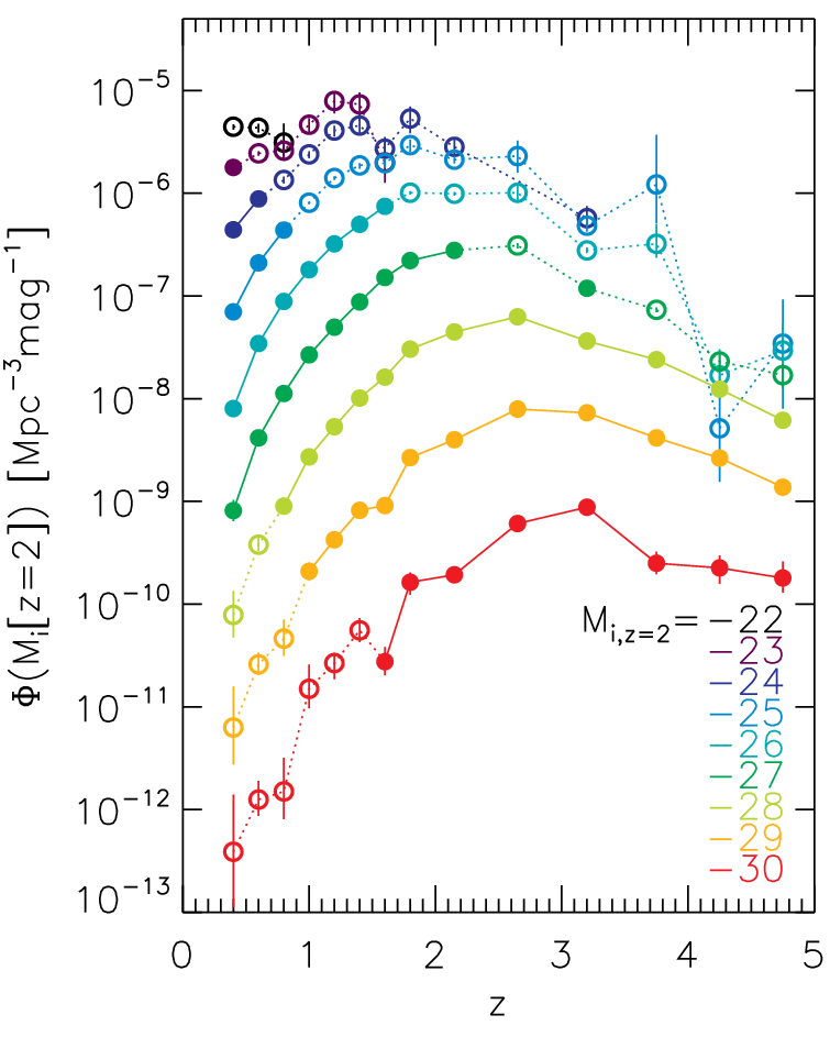
Fig. 15 shows the model LF in all 14 zbins. We only plot the portion that is above the flux limit in each individual bin for which our model LF reproduces the binned LF well and the constraints are the tightest. The width of each stripe indicates the 1 () range of the model LF. The dashed vertical line indicates , beyond which there is no binned LF data (see Fig. 13). The most noticeable feature is that the curvature of the LF changes significantly beyond . This is noted in Richards et al. [82] as the flattening of the bright-end slope, if a single power-law were fitted to the binned LF data. However, it appears to be more of a strong evolution of the break luminosity than a change in the bright-end slope. Recently, Fontanot et al. [26] argue that the apparent flattening in the bright-end slope is caused by an overestimation of the completeness of SDSS color selection at , as was adopted in Richards et al. [82]. An implicit assumption in their argument is that the completeness must become lower towards the flux limit, leading to an artificial flattening in the bright-end slope. However, we found that in our model LF, the break luminosity in the LF gradually increases towards higher redshift in a continuous fashion (see Fig. 15), and the slope is already significantly flattened at for . Thus it is not obvious that this flattening in the bright-end slope is caused by the possible differential incompleteness in the SDSS color selection. A more careful analysis is needed to resolve this issue.
Another notable feature is that zbin7 () shows a steeper slope at than the adjacent zbins. This is not caused by the failure of our model, as shown in Fig. 13. A close comparison between our model LF and the binned LF is shown in Fig. 16 for zbin6, zbin7 and zbin8. The points show the binned LF data, and the lines show the model LF from our Bayesian approach; the two are in excellent agreement. This apparent deviation in zbin7 is likely caused by the systematics of emission line -correction. For this zbin, the MgII line contributes the most to -band. The MgII line strength relative to the continuum decreases with luminosity [102, e.g., the Baldwin effect, Baldwin 1977; see fig. 13 in], thus using a constant emission line -correction in this bin will lead to more underestimated continuum luminosity towards the brighter end. This causes an artificial steepening at the bright end of the zbin7 LF (a similar effect is seen for zbin12 where CIV contributes the most to the -band). This is a second-order effect and therefore we do not correct for it in the present work. However, it does indicate that as the statistics becomes much better, additional systematic effects need to be taken into account in order to get unbiased results. We note that zbin7 also shows notable deviations from zbin6 and zbin8 in terms of the extrapolated LF and constraints on model parameters (see Figs. 11 and 13).
Finally, as mentioned earlier, the LF (above the SDSS flux limit) generally flattens (i.e., the luminosity break) at brighter magnitude towards higher redshift, consistent with earlier findings [17, e.g.,]. However, we did not observe a significant steepening of the bright-end slope from to , in tension with Croom et al. [17]. We suspect this discrepancy is caused by the different methods to measure the LF: Croom et al. [17] fit the LF with a broken power-law function, while our LF estimate is non-parametric.
Fig. 17 (left) shows the evolution of quasar number density as a function of luminosity, using our model LF. Filled circles indicate the portion of the LF that is sampled by SDSS quasars, and open circles indicates extrapolated model LF. Note that at low redshift, the SDSS sample also suffers from the bright cut, in addition to the faint luminosity cut. We only extrapolate the model LF to 3 magnitudes fainter, where our model constraints are still reasonably good. With the addition of extrapolated data, there is a clear trend that the number density of more luminous quasars peak earlier. Compared with the results from 2SLAQ+SDSS [17], our sample extends to higher redshift and the peaks for the bright quasars are well resolved.
Fig. 17 (right) shows the evolution of quasar number density as a function of BH mass. The uncertainties in each redshift bin are quite large, reflecting the poorly constrained BHMF (e.g., Fig. 14). However, there is tentative evidence that more massive BHs achieve their peak density earlier. This is the manifestation of “cosmic downsizing” in terms of BH mass. As redshift decreases, active BHs become on average less massive and are likely in less massive hosts. The number density of quasars peaks around , which is consistent with the trend found in §III.1 based on virial masses (although the characteristic BH mass shifted to for virial masses due to the luminosity-dependent bias in the flux limited sample). Kelly et al. [53] also found evidence for active BH mass downsizing, and Vestergaard & Osmer [124] found downsizing at the high-mass end of the active BHMF, although the latter did not correct for incompleteness and scatter in virial mass estimates.
We can compare the derived active BHMF with the local dormant BHMF estimated by Shankar et al. [94]. Below (the upper limit that can be measured for the local BHMF), the active BHMF at any redshift is always more than one order of magnitude lower than the local dormant BHMF. This means quasars are by no means a long-lived cosmological population, and we are witnessing different generations of quasars at different redshift, which cumulatively (over time) build up the local dormant BH population.
Fig. 18 further demonstrates the insignificant contribution of broad-line quasars to the total BH mass density at all redshifts. The black line shows the accreted BH mass density using the bolometric LF estimated by Hopkins et al. [42] and a radiative efficiency , where the gray shaded region is centered on the black line and has a vertical width of dex, which is a conservative estimate for the uncertainty in the accreted BH mass density due to uncertainties in the bolometric LF and radiative efficiency. The accreted BH mass density at is consistent with the estimated BH mass density using local spheroid-BH scaling relations [94, 137, e.g.,]. The black circles are the measured global stellar mass density in Pérez-González et al. [74], scaled by a factor of . Although there are systematic uncertainties in both the accreted BH mass density and the measured global stellar mass density, the agreement between the two is remarkable, and argues strongly for the co-evolution between galaxies and BHs. However, the total BH mass density in broad-line quasars (magenta circles), estimated by integrating over our model BHMF, is at least one order of magnitude less than the total BH mass density at all times.
V.2. The Eddington ratio distribution

Our model specifies the Eddington ratio distribution (or luminosity distribution) at fixed BH mass99 9 The Eddington ratio distribution at fixed BH mass is different from that at fixed luminosity, in the presence of scatter of the relation (cf. Fig. 8). This is true no matter which mass is used (virial versus true). For the virial mass-based Eddington ratio at fixed luminosity, the average value scales as from the virial relation (assuming a slope of in the mean relation). However, for the virial mass-based Eddington ratio at fixed virial mass, the average value has a much weaker dependence on , and one also must account for the selection effect of the flux limit. These points are well demonstrated in Fig. 8.. Even though the constrained parameters have large uncertainties (see Fig. 11), it appears that a linear relation between the mean luminosity and mass is consistent with the data. This means that the mean Eddington ratio does not depend on mass strongly. However, there is some evidence that the mean Eddington ratio increases with redshift, which may reflect the evolution of the average accretion efficiency or the general decline of quasar light curve. The scatter in the Eddington ratio distribution is poorly constrained, and no coherent redshift evolution is seen. Nevertheless, we found a median value of dex in the dispersion of Eddington ratios at fixed BH mass, consistent with earlier studies [97, 53, e.g.,].
The Eddington ratio distribution in any flux-limited sample or at fixed luminosity is essentially different from that of all broad-line quasars or at fixed BH mass, as emphasized in Shen et al. [97] and Kelly et al. [53]. It suffers from the Malmquist-type bias such that more high-Eddington ratio and low mass objects are scattered into the flux-limited sample than low-Eddington ratio and high mass objects scattered out (i.e., due to a non-zero and a bottom-heavy BHMF). Thus the average Eddington ratio is biased high in our sample. In addition, using virial masses can further modify the sample-averaged Eddington ratio due to the luminosity-dependent bias (i.e., a non-zero ).
Fig. 19 summarizes these behaviors. Plotted here are the sample-averaged Eddington ratio and its uncertainty1010 10 Note that the uncertainty here refers to the uncertainty in the mean Eddington ratio, not the scatter in Eddington ratio. in 14 zbins under different circumstances. The filled magenta squares are for all the broad-line quasars, and the open green squares are for those that are detectable above the flux limit; both are estimated using our model outputs. The difference between the mean Eddington ratio for all quasars and detectable quasars reflects the scatter in luminosity at fixed true mass () and the shape of the underlying BHMF, and in general the mean Eddington ratio in the detectable sample is biased high. The open triangles are for all quasars in our sample, where the Eddington ratios are estimated with virial BH masses. The difference between the mean Eddington ratio for the detectable quasars estimated with true masses and virial masses mostly reflects the luminosity-dependent bias (i.e., a non-zero ). Since we have a positive for most zbins, the mean Eddington ratio based on virial masses for the detectable quasars is generally biased low than the true value1111 11 When is small, the difference between the mean Eddington ratio with true masses and virial masses for the flux-limited sample may not be discernable, due to the slightly different calculations of the mean Eddington ratio in the two cases: the mean true Eddington ratio is calculated using random draws from the posterior distribution; the mean virial Eddington ratio is the median in the observed distribution. .
V.3. Model caveats and future perspectives
Our forward Bayesian modeling stands for a major improvement on retrieving information from the mass-luminosity plane compared with previous studies based on virial BH masses. However, there are still several caveats in our approach, which can be improved in future investigations:
- •
First and foremost, we assumed that the specific forms of single-epoch virial mass estimators adopted in this work give unbiased BH mass estimates when averaged over luminosity at fixed true mass, i.e., , where stands for the expectation value. While this is true for the local RM AGN sample (by calibration), it may not hold when extrapolating to the high-redshift and high-luminosity population.
Also, we recognize that different versions of virial estimators (even for the same line) do not necessarily yield the same BH masses. If the virial mass estimators that we used were already biased for objects in our sample (i.e., due to an imperfect virial calibration, or other generic systematics in the virial technique) then the BHMF estimation would also be biased. In particular, it is possible that FWHM is a worse indicator for the virial velocity than other line width measures [76, 14, 128, 77, 78, such as line dispersion, see arguments by], and the luminosity bias we found here may reflect the systemics with incorrect forms of virial estimators.
Nevertheless, there is currently no consensus on which versions of virial estimator are the best. As a proof of concept, our model can easily be adapted to use the updated virial calibrations when they become available. A similar study based on line dispersion-based virial BH masses is currently under way.
- •
Our parameterized model is still in a relatively restrictive form, especially for the the Eddington ratio model at fixed true mass. We have tested with rather relaxed parameterizations for the joint distribution of luminosity and true mass, but found that the current data is not sufficient to give reasonable constraints if we treat the luminosity-dependent bias as a free parameter. This can be seen in Fig. 8 that the current data only sample the tip of the distribution, and thus it is difficult to constrain parameters for overly flexible models. Deeper data is needed to test more flexible models. A fainter broad-line quasar sample, such as the 2SLAQ sample [17] or the BOSS quasar sample [84], will also provide more stringent constraints on our model parameters and better representation of the mass-luminosity plane.
Nevertheless, the capability of reproducing the observed distribution is reassuring that a single lognormal Eddington ratio model with a mass-dependent mean is still a reasonable choice. An alternative model would be a power-law Eddington ratio distribution at fixed true mass, as suggested in some models for the decaying part of the quasar light curve [136, 40, 96, e.g.,]. However, since quasars are continuously forming (especially for fainter quasars, whose number density peaks later in time), at each epoch we should also witness quasars in their rising part of the light curve, unless this period is completely obscured. In addition, the broad line region may only exist when the BH is accreting at high accretion rate during AGN evolution [99, 41, e.g.,], i.e., with Eddington ratio [120, e.g.,], and there must be fluctuations in the instantaneous Eddington ratio. Thus a lognormal model may indeed capture the basic characteristic of the Eddington ratio distribution at fixe BH mass.
In a follow-up paper (Kelly & Shen, in preparation), we will use a more generic prescription to model the joint distribution of luminosity and BH mass directly instead of using a specific Eddington ratio model as adopted here. This will be achieved at the cost of simplifying other prescriptions in the model, for instance, fixing the value of . However, by relaxing the single lognormal Eddington ratio model, we can test if a single lognormal model is a good approximation. It also allows a more proper investigation of the mass-luminosity plane.
Finally, we note that we assumed a Gaussian distribution for the error in the virial mass estimates (which may not be adequate), and our model is not robust to outliers. These issues may be partly responsible for the large uncertainties we get in several zbins. We plan to investigate these issues in future work.
- •
Since we are only concerned with broad-line objects, the active BHMF derived in this paper is a lower-limit for the active SMBH population. It is important to include the growth of SMBHs in obscured accretion or with accretion mode that does not produce broad lines, as traced by populations of active BHs selected by various other techniques [113, 79, 60, 117, 37, 20, 135, 134, 13, e.g.,]. This non-broad-line population could contribute as much as one half of the total accreted BH mass density, although significant uncertainty remains in determining their relative abundance to the broad-line population.
VI. Conclusions
This paper represents our first step towards a systematic investigation on the demographics of broad-line quasars in the mass-luminosity plane and its redshift evolution. We used a forward modeling Bayesian framework to model the joint distribution in the mass-luminosity plane. With simple model prescriptions for the underlying active BHMF and Eddington ratio distribution, we were able to fit the observed distribution above the sample flux limit and extrapolate below using constrained model parameters. We paid particular attention to the distinction between virial mass estimates and true masses, and corrected for the selection effects of flux limited samples. The main conclusions of the paper are the following:
- 1.
Virial BH masses are not true masses (§III.2.1), and their explicit dependence on luminosity has implications for their conditional probability distributions: , and . We found evidence that for MgII and possibly CIV, there is a positive luminosity-dependent bias in virial masses, such that at fixed true mass, objects with luminosities above average have over-estimated virial masses. This is expected as there must be uncorrelated scatter between line width and luminosity at fixed true mass, due to the imperfectness of them being the surrogates for the virial velocity and the BLR radius in the virial mass technique. While this bias was noted earlier [97, 98], this is for the first time that we quantified the level of this bias with the SDSS quasar sample. As a consequence, the dispersion in virial mass in narrow luminosity bins or flux-limited samples is generally smaller than the virial mass uncertainty [97, 98], and the average virial BH masses in SDSS quasars are likely overestimated by a factor of a few.
- 2.
Our model LF is tightly constrained in the regime sampled by SDSS quasars, and makes reasonable predictions when extrapolated magnitudes fainter, as compared with the LF measured from faint quasar surveys. Downsizing in LF evolution is clearly seen with our model LF. The break luminosity (as in a double power-law model) increases towards higher redshift. As a consequence, the LF slope for from a single power-law fit appears shallower at than at lower redshift.
- 3.
Except for a few zbins, the model active BHMF usually cannot be well constrained to within a factor of a few. This is mainly caused by the additional free parameter on the luminosity-dependent bias, which leads to degeneracies with other parameters. The SDSS sample only probes the tip of the active SMBH population at high redshift, which makes it more difficult to constrain model parameters for the whole population. Nevertheless, the abundance of the most massive quasars is always overestimated using virial masses regardless of the luminosity-dependent bias. Within our model a turn-over at the low-mass end of the true BHMF is needed in order to fit the observed distribution in the mass-luminosity plane, but we caution that this result is based on our model assumptions and may suffer from the poor sampling of low-mass BHs in the SDSS sample. Further investigations are needed to test the robustness of this feature. This turn-over shifts to larger BH masses for the detected population in SDSS due to the flux limit. Although with large error bars, we found tentative evidence that downsizing also manifests itself in the active BHMF, and the number density of quasars peaks around .
The total BH mass density in broad-line quasars is always insignificant compared with that in all SMBHs at any redshift (Fig. 18).
- 4.
Within our model uncertainties, the Eddington ratio distribution at fixed true BH mass has a mean value that weakly depends on mass, and an average scatter of dex. The sample-averaged Eddington ratio for all broad-line quasars ranges between and , and increases with redshift (Fig. 19). The sample-averaged Eddington ratio for quasars above the SDSS flux limit is Malmquist-biased due to the scatter in Eddington ratios at fixed BH mass and the shape of the underlying active BHMF. Furthermore, using virial masses for the detected quasars tend to reduce the Eddington ratio again due to the luminosity-dependent bias (Fig. 19).
- 5.
Our model reproduces the observed distribution in the mass-luminosity plane (with virial masses). The flux limit, the scatter between true masses and virial masses, as well as the luminosity-dependent bias, change the distribution in the mass-luminosity plane significantly. Thus any features in the mass-luminosity plane based on virial masses must be interpreted with caution.
Our results highlight the need for understanding the systematics in the virial mass technique. All single-epoch virial mass estimators currently utilized in the literature are bootstrapped from the local RM AGN sample of only several dozen objects. These mass estimators have been extensively used for high redshift and high luminosity quasars, a regime that is poorly sampled by RM AGNs. We have shown that even without other systematic issues with the virial technique, the scatter and luminosity-dependent bias between virial masses and true masses already make it difficult to constrain the active BHMF accurately. Any additional systematic issues will simply make the situation worse.
Since BH mass is a crucial physical quantity and is related to many fundamental processes of SMBHs, refining the techniques that weigh the BH is of tremendous importance. As the most promising method to measure active BH masses, the RM technique (and its extensions of single-epoch virial estimators) should be tested and calibrated carefully. Progress is being made in reverberation mapping studies of broad-line AGNs and calibrations of virial mass estimators [48, 8, 132, 30, e.g.,], as well as in the statistical description of AGN variability as applied to reverberation mapping [140, 12, 73, e.g.,]. However, to fully understand the BLR kinematics/geometry and to construct reliable mass estimators, a substantially larger RM sample is needed to sample an unbiased parameter space of broad-line objects, as well as a much better understanding of the systematics in the RM technique and single-epoch mass estimators.
References
- [1] Assef, R. J., et al. 2011, ApJ, 742, 93
- [2] Babić, A., Miller, L., Jarvis, M. J., Turner, T. J., Alexander, D. M., & Croom, S. M. 2007, A&A, 474, 755
- [3] Baldwin, J. A. 1977, ApJ, 214, 679
- [4] Barger, A. J., Cowie, L. L., Mushotzky, R. F., Yang, Y., Wang, W.-H., Steffen, A. T., & Capak, P. 2005, AJ, 129, 578
- [5] Baskin, A., & Laor, A. 2005, MNRAS, 356, 1029
- [6] Bentz, M. C., Peterson, B. M., Pogge, R. W., Vestergaard, M., & Onken, C. A. 2006, ApJ, 644, 133
- [7] Bentz, M. C., Peterson, B. M., Netzer, H., Pogge, R. W., & Vestergaard, M. 2009a, ApJ, 697, 160
- [8] Bentz, M. C., et al., 2009b, ApJ, 705, 199
- [9] Blandford, R. D., & McKee, C. F. 1982, ApJ, 255, 419
- [10] Bongiorno, A., et al. 2007, A&A, 472, 443
- [11] Boyle, B. J., Shanks, T., Croom, S. M., Smith, R. J., Miller, L., Loaring, N., & Heymans, C. 2000, MNRAS, 317, 1014
- [12] Brewer, B. J., et al. 2011, ApJ, 733, L33
- [13] Civano, F., et al. 2011, ApJ, 741, 91
- [14] Collin, S., Kawaguchi, T., Peterson, B. M., & Vestergaard, M. 2006, A&A, 456, 75
- [15] Cowie, L. L., Barger, A. J., Bautz, M. W., Brandt, W. N., & Garmire, G. P. 2003, ApJ, 584, L57
- [16] Croom, S. M., Smith, R. J., Boyle, B. J., Shanks, T., Miller, L., Outram, P. J., & Loaring, N. S. 2004, MNRAS, 349, 1397
- [17] Croom, S. M., et al. 2009, MNRAS, 399, 1755
- [18] Denney, K. D., Peterson, B. M., Dietrich, M., Vestergaard, M., & Bentz, M. C. 2009, ApJ, 692, 246
- [19] Eddington, A. S. 1913, MNRAS, 73, 359
- [20] Elvis, M., et al. 2009, ApJS, 184, 158
- [21] Fan, X., et al. 2001, AJ, 121, 54
- [22] —. 2004, AJ, 128, 515
- [23] Ferrarese, L., & Merritt, D. 2000, ApJ, 539, L9
- [24] Fine, S., et al. 2008, MNRAS, 390, 1413
- [25] —. 2010, MNRAS, 409, 591
- [26] Fontanot, F., Cristiani, S., Monaco, P., Nonino, M., Vanzella, E., Brandt, W. N., Grazian, A., & Mao, J. 2007, A&A, 461, 39
- [27] Gavignaud, I., et al. 2008, A&A, 492, 637
- [28] Gebhardt, K., et al. 2000, ApJ, 539, L13
- [29] Glikman, E., Djorgovski, S. G., Stern, D., Dey, A., Jannuzi, B. T., & Lee, K.-S. 2011, ApJ, 728, L26
- [30] Graham, A. W., Onken, C. A., Athanassoula, E., & Combes, F. 2011, MNRAS, 412, 2211
- [31] Green, R. F., Schmidt, M., & Liebert, J. 1986, ApJS, 61, 305
- [32] Greene, J. E., & Ho, L. C. 2007, ApJ, 667, 131
- [33] Gültekin, K., et al. 2009, ApJ, 698, 198
- [34] Haiman, Z., & Loeb, A. 1998, ApJ, 503, 505
- [35] Hao, L., et al. 2005, AJ, 129, 1795
- [36] Hasinger, G., Miyaji, T., & Schmidt, M. 2005, A&A, 441, 417
- [37] Hickox, R. C., et al. 2009, ApJ, 696, 891
- [38] Hopkins, P. F., Hernquist, L., Cox, T. J., Di Matteo, T., Robertson, B., & Springel, V. 2006, ApJS, 163, 1
- [39] Hopkins, P. F., Hernquist, L., Cox, T. J., & Kereš, D. 2008, ApJS, 175, 356
- [40] Hopkins, P. F., Hernquist, L., Martini, P., Cox, T. J., Robertson, B., Di Matteo, T., & Springel, V. 2005, ApJ, 625, L71
- [41] Hopkins, P. F., Hickox, R., Quataert, E., & Hernquist, L. 2009, MNRAS, 398, 333
- [42] Hopkins, P. F., Richards, G. T., & Hernquist, L. 2007, ApJ, 654, 731
- [43] Ikeda, H., et al. 2011, ApJ, 728, L25
- [44] Jiang, L., et al. 2006, AJ, 131, 2788
- [45] Jiang, L., Fan, X., Vestergaard, M. , Kurk, J. D., Walter, F., Kelly, B. C., & Strauss, M. A., 2007, AJ, 134, 1150
- [46] Jiang, L., et al., 2008, AJ, 135, 1057
- [47] Jiang, L., et al., 2009, AJ, 138, 305
- [48] Kaspi, S., Brandt, W. N., Maoz, D., Netzer, H., Schneider, D. P., & Shemmer, O. 2007, ApJ, 659, 997
- [49] Kaspi, S., Smith, P. S., Netzer, H., Maoz, D., Jannuzi, B. T., & Giveon, U. 2000, ApJ, 533, 631
- [50] Kauffmann, G., & Haehnelt, M. 2000, MNRAS, 311, 576
- [51] Kelly, B. C. 2007, ApJ, 665, 1489
- [52] Kelly, B. C., Vestergaard, M., & Fan, X. 2009, ApJ, 692, 1388
- [53] Kelly, B. C., Vestergaard, M., Fan, X., Hopkins, P., Hernquist, L., & Siemiginowska, A. 2010, ApJ, 719, 1315
- [54] Kelly, B. C., & Bechtold, J. 2007, ApJS, 168, 1
- [55] Kollmeier, J. A., et al. 2006, ApJ, 648, 128
- [56] Krolik, J. H. 2001, ApJ, 551, 72
- [57] Kurk, J. D., et al., 2007, ApJ, 669, 32
- [58] Labita, M., Decarli, R., Treves, A., & Falomo, R. 2009, MNRAS, 396, 1537
- [59] Lauer, T. R., Tremaine, S., Richstone, D., & Faber, S. M. 2007, ApJ, 670, 249
- [60] Luo, B., et al. 2008, ApJS, 179, 19
- [61] Lynden-Bell, D. 1969, Nature, 223, 690
- [62] Magorrian, J., et al. 1998, AJ, 115, 2285
- [63] Malmquist, K. G. 1922, Lund Medd. Ser. I, 100, 1
- [64] Marconi, A., Axon, D. J., Maiolino, R., Nagao, T., Pastorini, G., Pietrini, P., Robinson, A., & Torricelli, G. 2008, ApJ, 678, 693
- [65] Marconi, A., Risaliti, G., Gilli, R., Hunt, L. K., Maiolino, R., & Salvati, M. 2004, MNRAS, 351, 169
- [66] McLure, R. J., & Dunlop, J. S. 2004, MNRAS, 352, 1390
- [67] McLure, R. J., & Jarvis, M. J. 2002, MNRAS, 337, 109
- [68] Merloni, A. 2004, MNRAS, 353, 1035
- [69] Merloni, A., & Heinz, S. 2008, MNRAS, 388, 1011
- [70] Netzer, H., Lira, P., Trakhtenbrot, B., Shemmer, O., & Cury, I. 2007, ApJ, 671, 1256
- [71] Netzer, H. 2009, ApJ, 695, 793
- [72] Onken, C. A., et al. 2004, ApJ, 615, 645
- [73] Pancoast, A., Brewer, B. J., & Treu, T. 2011, ApJ, 730, 139
- [74] Pérez-González, P. G., et al. 2008, ApJ, 675, 234
- [75] Peterson, B. M. 1993, PASP, 105, 247
- [76] Peterson, B. M., et al. 2004, ApJ, 613, 682
- [77] Rafiee, A., & Hall, P. B. 2011a, MNRAS, 825
- [78] Rafiee, A., & Hall, P. B. 2011b, ApJS, 194, 42
- [79] Reyes, R., et al. 2008, AJ, 136, 2373
- [80] Richards, G. T., et al. 2002, AJ, 123, 2945
- [81] —. 2005, MNRAS, 360, 839
- [82] —. 2006, AJ, 131, 2766
- [83] —. 2011, AJ, 141, 167
- [84] Ross, N. P., et al. 2011, arXiv:1105.0606
- [85] Salpeter, E. E. 1964, ApJ, 140, 796
- [86] Salucci, P., Szuszkiewicz, E., Monaco, P., & Danese, L. 1999, MNRAS, 307, 637
- [87] Schmidt, M. 1963, Nature, 197, 1040
- [88] Schmidt, M. 1968, ApJ, 151, 393
- [89] Schmidt, M., & Green, R. F. 1983, ApJ, 269, 352
- [90] Schafer, C. M. 2007, ApJ, 661, 703
- [91] Schneider, D. P., et al. 2010, AJ, 139, 2360
- [92] Schulze, A., & Wisotzki, L. 2010, A&A, 516, 87
- [93] Shankar, F., Salucci, P., Granato, G. L., De Zotti, G., & Danese, L. 2004, MNRAS, 354, 1020
- [94] Shankar, F., Weinberg, D. H., & Miralda-Escudé, J. 2009, ApJ, 690, 20
- [95] Shankar, F., Crocce, M., Miralda-Escude’, J., Fosalba, P., & Weinberg, D. H. 2010, ApJ, 718, 231
- [96] Shen, Y. 2009, ApJ, 704, 89
- [97] Shen, Y., Greene, J. E., Strauss, M. A., Richards, G. T., & Schneider, D. P. 2008, ApJ, 680, 169
- [98] Shen, Y., & Kelly, B. C. 2010, ApJ, 713, 41
- [99] Shen, Y., Mulchaey, J. S., Raychaudhury, S., Rasmussen, J., & Ponman, T. J. 2007a, ApJ, 654, L115
- [100] Shen, Y., et al. 2007b, AJ, 133, 2222
- [101] —. 2009, ApJ, 697, 1656
- [102] —. 2011, ApJS, 194, 45
- [103] Silverman, J. D., et al. 2005, ApJ, 624, 630
- [104] Silverman, J. D., et al. 2008, ApJ, 679, 118
- [105] Small, T. A., & Blandford, R. D. 1992, MNRAS, 259, 725
- [106] Soltan, A. 1982, MNRAS, 200, 115
- [107] Somerville, R. S., Hopkins, P. F., Cox, T. J., Robertson, B. E., & Hernquist, L. 2008, MNRAS, 391, 481
- [108] Steffen, A. T., Barger, A. J., Cowie, L. L., Mushotzky, R. F., & Yang, Y. 2003, ApJ, 596, L23
- [109] Steinhardt, C. L. 2011, ApJ, 738, 110
- [110] Steinhardt, C. L., & Elvis, M. 2010a, MNRAS, 402, 2637
- [111] —. 2010b, MNRAS, 406, L1
- [112] Steinhardt, C. L., Elvis, M., & Amarie, M. 2011, MNRAS, 415, 732
- [113] Stern, D., et al. 2005, ApJ, 631, 163
- [114] Sulentic, J. W., Bachev, R., Marziani, P., Negrete, C. A., & Dultzin, D. 2007, ApJ, 666, 757
- [115] Sulentic, J. W., Repetto, P., Stirpe, G. M., Marziani, P., Dultzin-Hacyan, D., & Calvani, M. 2006, A&A, 456, 929
- [116] Trakhtenbrot, B., Netzer, H., Lira, P. & Shemmer, O. 2011, ApJ, 730, 7
- [117] Treister, E., et al. 2009, ApJ, 706, 535
- [118] Tremaine, S., et al. 2002, ApJ, 574, 740
- [119] Trump, J. R., et al. 2009, ApJ, 700, 49
- [120] Trump, J. R., et al. 2011, ApJ, 733, 60
- [121] Ueda, Y., Akiyama, M., Ohta, K., & Miyaji, T. 2003, ApJ, 598, 886
- [122] Vestergaard, M. 2004, ApJ, 601, 676
- [123] Vestergaard, M., Fan, X., Tremonti, C. A., Osmer, P. S., & Richards, G. T. 2008, ApJ, 674, L1
- [124] Vestergaard, M., & Osmer, P. S. 2009, ApJ, 699, 800
- [125] Vestergaard, M., & Peterson, B. M. 2006, ApJ, 641, 689
- [126] Volonteri, M., Haardt, F., & Madau, P. 2003, ApJ, 582, 559
- [127] Wandel, A., Peterson, B. M., & Malkan, M. A. 1999, ApJ, 526, 579
- [128] Wang, J., et al. 2009, ApJ, 707, 1334
- [129] Willott, C. J., et al., 2010, AJ, 140, 546
- [130] Willott, C. J., et al., 2010, AJ, 139, 906
- [131] Wolf, C., Wisotzki, L., Borch, A., Dye, S., Kleinheinrich, M., & Meisenheimer, K. 2003, A&A, 408, 499
- [132] Woo, J.-H., et al. 2010, ApJ, 716, 269
- [133] Wyithe, J. S. B., & Loeb, A. 2003, ApJ, 595, 614
- [134] Xue, Y. Q., et al. 2011, ApJS, 195, 10
- [135] Yan, R., et al. 2011, ApJ, 728, 38
- [136] Yu, Q., & Lu, Y. 2004, ApJ, 602, 603
- [137] —. 2008, ApJ, 689, 732
- [138] Yu, Q., & Tremaine, S. 2002, MNRAS, 335, 965
- [139] Zel’dovich, Y. B., & Novikov, I. D. 1964, Dokl. Akad. Nauk SSSR, 158, 811
- [140] Zu, Y., Kochanek, C. S., & Peterson, B. M. 2011, ApJ, 735, 80
*