Tevatron Top Versus LHC Top Physics
Abstract
We carry out a comprehensive analysis of models for top at CDF in light of new top data arriving from the LHC. We begin with a careful Tevatron analysis, considering in general which sets of effective vertices give rise to a large forward-backward asymmetry while suppressing the contribution to the total cross-section. We show on general grounds that scalar models struggle to produce sufficient asymmetries consistent with CDF observations, while vector models can produce a large asymmetry with a less significant tension in the total cross-section and invariant mass distribution at the Tevatron. We examine the essential observables of these models for top physics at LHC7 with of data, including the total cross-section, invariant mass distribution and number of additional jets in events. In the case of -channel mediators, the LHC total cross-section places a strong constraint on light mediators, while the Tevatron invariant mass distributions place strong constraints on heavy mediators that are able to produce the asymmetry. Heavy axigluons are becoming increasingly squeezed by LHC7 and dijet resonance searches. We conclude that LHC7 top analyses are rapidly closing the window for viable models of the CDF top .
I Introduction
The Large Hadron Collider (LHC) is providing an unprecedented probe of top quark properties. While the Tevatron has to date collected on the order of a thousand tops, the LHC, with of data has already nearly an order of magnitude more tops. The improvement is due both to a larger production cross-section, and to improved rapidity coverage for leptons in semi-leptonic and fully leptonic top analyses. In terms of the percentage error on the total cross-section, the 7 TeV LHC (LHC7) results are already competitive with the Tevatron [1] with only [2], while the invariant mass distribution with just extends to a higher of 2.5 TeV [3] as compared to the Tevatron reach of 1.8 TeV [4]. At , the top quark properties will be far better measured than at the Tevatron.
At the same time, the Tevatron as a machine is better able at the outset to measure a forward-backward asymmetry.11 1 Though see [5, 6] for efforts to make a measurement of the forward-backward asymmetry at the LHC. The asymmetry in a particular invariant mass bin, , is defined by
| (1) |
with the rapidity difference between a top and an anti-top. The recent CDF anlaysis shows for GeV [7] at the parton level (or at the signal level)22 2 Throughout this paper we use “signal level” to refer to background subtracted, raw measured quantities in the detector, and “parton level” to refer to unfolded results which attempt to subtract detector effects from the results., while the Next-to-Leading Order (NLO) Standard Model (SM) predicts much lower values (or at the signal level) [8, 9, 10, 11, 12], corresponding to a 3.4 deviation (3.6 at signal level). A measurement of the asymmetry with fully leptonic tops has also been made which is roughly consistent with the measurement in the semileptonic channel [13]. The D0 collaboration also observes a larger than predicted asymmetry [14].
Because this asymmetry is so large, any new physics (NP) that could generate such an asymmetry must have large couplings to the top as well as to the light quarks in the initial state. A very large number of models have been proposed in the literature. However, from a phenomenological point of view, these models mainly fall into only two categories according to the nature of the new particle exchange: (i) -channel exchange of vector mediators (e.g. axigluon models) [15, 16, 17, 18, 19, 20, 21, 22, 23, 24, 25, 26, 27, 28, 29, 30, 31, 32, 33, 34, 35] or (ii) -channel exchange of flavor-violating mediators [36, 37, 38, 40, 39, 41, 42, 43, 44, 45, 46, 47, 48, 49, 50, 51, 52]33 3 There is another class of models that can create effective axial QCD coupling from NP [53]. . Comparative studies of these models have also been carried out [54, 55, 56, 57, 58, 59, 60, 61], and their implications for top observables at the Tevatron observed [61, 62]. The -channel mediators often have maximally axial couplings (though there are exceptions such as [35]), while the -channel mediators connect a light quark to the top quark in a way that appears to maximally violate flavor. A number of studies on the implications of these models for LHC physics have also been carried out [45, 63, 64, 65, 66].
There are a large number of possibilities for the spin, color, flavor and electroweak representation of a new field that fits into the two categories mentioned above. In the literature these have been mostly built and studied one by one. Here, by contrast, we are motivated to extract general features to determine which effective vertices are able to generate the large while contributing a small amount to the total cross-section. We find that the form of the matrix element itself allows one to make general conclusions about which classes of models are successful in generating a significant asymmetry.
We find on general grounds that perturbative44 4 Scalar models with larger couplings can achieve larger asymmetries, though at the expense of a larger contribution to the total cross-section. scalar models typically can produce no more than a “parton level” asymmetry for , which is only somewhat larger than the asymmetry produced in the SM (at ) and well below CDF’s parton level central value of .55 5 The data-level asymmetry yields a result about a factor of two lower than the parton level result, which has been confirmed by the theoretical study of [61]. A comparison of a parton level theoretical result to the signal level asymmetry is not valid, and will underproduce by more than the observed asymmetry. The reason is simply the combination of the Mandelstam variables that enters into - and -channel processes for scalars; the statement is independent of the color (singlet, triplet, sextet or octet) or flavor representation of the state. By contrast, -channel vectors have a matrix element that is conducive to producing a large asymmetry with a relatively small contribution to the total cross-section.
We systematically enumerate the possibilities for the quantum numbers of - and - channel mediators that can produce an asymmetry and show that classes of models are strongly disfavored based on a small contribution to the total asymmetry or large contribution to the total cross-section at the Tevatron. This paper is intended to be a companion to our earlier paper on [61], which carried out a systematic comparison of NP models to the data. This was the only theory paper to carry out the full top reconstruction in order to compare results at the signal level. We found that there were large acceptance effects which changed the extracted parton level comparison between the SM and the NP models.66 6 See also [50] for a discussion of the acceptance effect at the parton level.
With LHC data quickly arriving, however, the source of strong constraints is rapidly changing, and we are particularly compelled by the fact that the LHC collaborations are now analyzing unprecedented amounts of top data that will clearly rule out a large swath of models. We examine observables from the LHC, such as total cross-section, invariant mass distribution, and the number of additional jets in events. In order to carry out our analysis, we have done a systematic scan in mass and coupling space for a broad class of models, described in appendix B. For a subset of the models that give the best fit to the data we generate 5 million events, applying cuts and reconstruction mirroring the ATLAS analysis [3] in order to compare to LHC distributions. Many models will be strongly constrained by these analyses with just .77 7 These statements must take into consideration, however, uncertainties in next-to-leading-order (NLO) corrections to the NP contributing to the total cross-section and invariant mass distribution. In our earlier paper on searching for flavor-violating resonances at the LHC, we proposed top-jet resonances as a means to search for -channel mediators [63]. Such a search is complementary to the analysis here. Many -channels models will be constrained by existing analyses, but the models that survive can have an imprint in top-jet resonances.
The outline of this paper is as follows. In the next section we discuss the classes of models that could generate the forward-backward asymmetry at the parton level, examining the asymmetries that are generated by the possible effective vertices, and drawing conclusions about which classes of models are viable. The reader who is interested only in the numerical results can skip this section, and move on to Sec. III, referring to Sec. (II) solely for a discussion of our conventions. In Sec. (III), we carry out a systematic scan of models at the Tevatron, choosing a set of models as benchmarks for simulation of the large data sets necessary for invariant mass distributions. In Sec. (IV), we then examine the expected top properties at the LHC for the classes of models we consider. In the appendices, parton level asymmetries, as well as a detailed discussion of our analysis pipeline, can be found.
II Effective Vertices and Top
Broadly speaking, either -channel or - (or )-channel resonances can generate the top forward-backward asymmetries at tree level. We show the diagrams that contribute both to the Tevatron and production at LHC in Fig. 1. The structure of the differential cross-section for models that produce the asymmetry through -channel exchange of a top-flavor-carrying mediator takes the same basic form according to whether the mediator is spin-0 or spin-1. Let the effective Lagrangian involving top and up quarks take the form
| (2) |
where for singlets and octets and for anti-triplets and sextets, and are the color generators of a representation — Hermitian matrices that contain Clebsch-Gordon coefficients connecting two (anti-)quarks, normalized so that . For singlets, we take . Note that we are restricting ourselves to couplings to top and up quarks, though our results should not qualitatively change given couplings to down-type quarks. We also only consider single mediator production; double mediator production is only important for light colored states, which are not present for the models we consider.
A large number of models of NP can generate these effective vertices, involving, in addition to the color group, potentially and flavor representations. There are a limited number of flavor symmetric models that can generate the top in the channel while satisfying existing constraints. We show in Table 1 the possibilities. There are also interactions that connect to , but these models with flavor symmetries are typically highly constrained by light quark observables since they mix with SM CKM physics. We do not consider them further. Interactions connecting, e.g., to through a spin-1 color triplet or sextet “diquark” are also possible, but as we will soon see (see Fig. 6), the dominant -channel interaction for top does not give rise to a significant positive asymmetry. We refer the reader to [67, 68] for a complete tabulation in the scalar mediator case of the possible flavor symmetries and to [46, 69] for discussion of in the context of Minimal Flavor Violation. In any case, the general observations that we make on the basis of the effective vertices in Eq. (2) will be relatively independent of the flavor representation, and we make the appropriate qualifications where necessary. For example, in flavor symmetric models, states in both the channel and the channel can contribute to the total asymmetry. Scalars in the channel don’t contribute to the forward-backward asymmetry, but can have an impact through their interference with -channel scalars that do generate the asymmetry.
| Interaction | Flavor () | |||
| 1, 8 | 2 | |||
| 1 | -4/3 | |||
| 1 | -1/3 | |||
| 1 | 0 | |||
| 1 | 0 | |||
| 1 | -1 |
Given the large number of possible combinations of - and -channel resonances from the flavor symmetric models, one despairs of ever being able to derive the characteristics of the state that can generate the asymmetry. However, we will find that in the (or ) channel, the amplitudes have very distinctive shapes dependent on whether the state is a vector or scalar mediator particle. We examine these characteristic features, and use it to draw conclusions about the nature of the mediator from the invariant mass dependence of . These conclusions are robust independent of the particular flavor symmetric model that one employs, and allows one to make general statements on the types of characteristics that are necessary for generating a large top .
The cross-sections arising from the NP interactions (2) and SM interactions are given by
| (3) |
| (4) |
| (5) |
and
| (6) |
Here and are color factors depending on the color rep of the mediator.88 8 Specifically, and where and for octets and singlets (anti-triplets and sextets). We have also defined
| (7) |
| (8) |
The Mandelstam variables are related to the scattering angle via
| (9) |
Note that we have not taken into account interference between NP contributions which can arise in flavor symmetric models. For example, -channel flavor conserving and -channel flavor changing diagrams may interfere. These new contributions do not give rise to any new types of terms (modulo mass terms in propagators) in the interference amplitude for the vector states, but do give rise to new contributions for the scalar states. We discuss these terms later, but suffice for now to comment that the new terms will not change our qualitative conclusions.
| Color rep: | 1 | 8 | 6 | |
|---|---|---|---|---|
| 4 | -2/3 | 1 | -1 | |
| 9 | 2 | 3/4 | 3/2 |
A flavor-conserving vector can give rise to an asymmetry at tree level if couplings to top and up have nonzero axial parts. Given the NP interaction Lagrangian
| (10) |
the scattering cross-sections calculated through these interactions are [56]:
| (11) |
and
| (12) |
where
| (13) |
For a color singlet rather than a color octet, the interference term vanishes and the squared term is scaled by a factor .
We now assemble these results using the parton distribution functions to gain a strong quantitative understanding of which types of interactions can give rise to the observed forward-backward asymmetry. The cross-section for the process is given by:
| (14) |
We define
| (15) |
Then the differential cross-section as a function of parton energy can be expressed as
| (16) |
Of course, all the dependence is in the parton-level differential cross-section. If only one kind of initial state parton contributes to the cross-section, then the PDF completely factors out of the differential forward-backward asymmetry, defined as a function of by
| (17) |
where
| (18) |
Suppose we are interested in a NP model with a nonzero contribution to the cross-section term generated through . We may then write the forward-backward asymmetry as a function of as
| (19) |
where
| (20) |
and is shown in Fig. (2). We note here that the falling SM contribution alone is not enough to give as steep a rise in the asymmetry as a function of as is observed at CDF. The rise can steepen through a combination of the following factors: (1) rises as a function of and/or (2) is comparable to the SM contribution and decreases as a function of . However, if the majority of the steepness were to come from mechanism (2), the total cross-section especially at low invariant mass would have to be comparable to the SM cross-section; this is hard to do without running into constraints on the total differential cross-section. Thus a significant contribution must come from .
There are seven kinds of terms that show up in a general cross-section involving -channel mediators, including its interference with the SM:
| (21) |
with for or -channel diquarks. We examine these contributions term by term to determine which types can successfully generate a large contribution. In particular, there must be a large contribution to the asymmetry with a very modest contribution to the total cross-section. That is to say simply that the odd contribution must be large in comparison to the even contribution.
We examine this in detail in Fig. (3) for different types of effective vertices. The salient points to take away from the figures are: (1) Scalars have odd contributions comparable to vectors only in the higher mediator mass range. (2) As a function of energy, the magnitude of the odd term for a given contribution is never greater than the magnitude of the even term, though some terms obtain much closer to equal magnitudes than others. Thus in order to best succeed in generating a sizable positive asymmetry while not destroying the invariant mass distribution, an ideal model will involve destructive interference between the even parts of the SM-NP interference and NP squared terms of the amplitude, and minimal or constructive interference between the odd part of the SM-NP interference and NP squared terms.99 9 That some amount of destructive interference is favored by the data was noted in [46]. By inspection, none of the scalars ( or -channel) can satisfy this condition. Scalar diquarks have some success in generating a substantial asymmetry in an intermediate mass range where the squared term contributes the dominant positive odd contribution. For the triplet, the interference term gives a negative odd and even contribution (so it helps to lower the cross-section but also lowers the numerator) while for the sextet the interference term enters with a minus sign and so gives a positive odd and even contribution (so it increases the numerator but also the cross-section).
For vectors there are more terms in play, so the story is a bit more complicated. To show the effects on the total asymmetry, we plot the total asymmetry (and, when relevant, cross-sections) for all - and -channel mediator color representations and spin combinations in Figs. (4)-(6). We show three benchmark mediator masses. Fig. (4) shows the scalar models that succeed in generating a positive asymmetry, though in general for perturbative couplings it is not a large positive asymmetry; Fig. (5) shows the same for the vector mediator case, and it is seen that the contribution to the total asymmetry can be large for all mass ranges. Lastly, we show in Fig. (6) the mediators that fail to produce a positive asymmetry larger than 5%. These include the scalar color octet and vector triplet and sextet.
One might wonder whether the asymmetry induced by scalars could be enhanced by adding another scalar with -channel couplings to and . This is predicted, for example, by the flavor triplet models. Interference between a -channel scalar with mass and an -channel scalar with mass would give rise to terms of the form and . These contributions, assuming , are shown in Fig. (7). For mediators lighter than the top quark, the odd contribution has the same sign as even for both terms, and it is hard to see how these contributions can enhance the asymmetry while not increasing the total cross-section to unacceptable levels. For mediators heavier than the top quark, odd and even contributions for the have the opposite sign—the odd contribution is positive for energies below the mediator mass and negative above. This interference could have interesting implications for models involving both -channel and -channel scalars of intermediate mass. Diquarks with -channel interactions would not contribute to the cross-section or .
Lastly, we briefly discuss -channel mediators, which can give rise to a large asymmetry for an appropriate choice of couplings and masses. If the asymmetry is generated from -channel NP interactions, then the dependence of the NP cross-section is a simple quadratic polynomial. The axigluon originally proposed in Ref. [18, 19] supposed a heavy axigluon to evade dijet and resonance searches that strongly constrain the state with masses below . However, recently different regions of the axigluon parameter space have been explored. For example, a 750 GeV state was considered in [35], with the dijet constraints evaded by making the coupling to the top quark much larger than to the up quarks. A 400 GeV state was considered in [31], and the resonance search constraints evaded by making the state sufficiently broad. Lastly, if a vector with diagonal axial couplings to top and up has a mass slightly lighter than the top mass, then it will not show up as a resonance in the spectrum. We refer the reader to these references for details, though we include the axigluons in our scans of parameter space in the next section for completeness.
III Comprehensive Search for Models at the Tevatron
To augment the conclusions of the previous section, we carry out a comprehensive representative scan of models using MadGraph[70]; the details of our procedure are discussed in Appendix B. We scan over -channel models, characterized by a single new mediator of given spin and color representation (2); we scan over all such models that can produce a positive asymmetry of more than a few percent while remaining (somewhat) perturbative (coupling ) and contributing less than order 50% to the total cross-section in the mass range 200 GeV - 2 TeV.1010 10 We neglect models with mass below the top (e.g. [50]); in general, these models will tend to rather severely overproduce the total cross-section and number of additional jets at the LHC and/or lead to large contributions to single top production, depending on the details of the mediator decay channels. The models scanned are summarized in Table 3. We choose representative models that generate the largest asymmetry. For -channel models we focus on mediators connecting up to top, both because they generate a large asymmetry, and also because a light neutral state runs into few constraints. The color singlet and triplet are our representative scalar models, though neither is successful in generating a large asymmetry, as we detailed earlier. Also note that the singlet scalar is part of an electroweak doublet, though we choose to couple this scalar to so that only one state is operative for the forward-backward asymmetry. The charged component of the mediator multiplet will contribute to plus jet events at the LHC, but this will be easily overwhelmed by the background. For the -channel flavor-violating models, we consider both a color singlet vector (C1V) and octet vector (C8V) that couples only to right-handed states. We also consider a flavor octet, color singlet vector (F8C1V) that couples to , where now the up quarks are in an octet of . Lastly, the -channel axiglue type models are considered, both in flavor universal [31] and non-universal [19, 35] varieties.
| Model | Spin | Color | Flavor | -, -, -? | Comments and References | |
|---|---|---|---|---|---|---|
| C1S | 0 | 1 | 1 | Only very moderate asymmetries achievable . Low mass () states do slightly better [51]. | ||
| C3S | 0 | 3 | 1 | a.k.a. triplet diquark. [38]. | ||
| C1V | 1 | 1 | 1 | a.k.a. or [50]. | ||
| C8V | 1 | 8 | 1 | |||
| F8C1V | 1 | 1 | 8 | , | Flavor breaking only through up Yukawa [46]. | |
| schanC8V(A,R) | 1 | 8 | 1 | a.k.a. axigluon or coloron. For , very broad width required to avoid resonance searches [19, 56, 35]. | ||
| schanC8V | 1 | 8 | 1 | GeV broad resonance via additional scalars. Universal quark couplings [31]. |
The results of this scan for the Tevatron are shown in Figs. (8) - (10). The coupling conventions in the figures are as follows. The -channel scalars, as well as C1V and C8V, models are labeled by their coupling to RH quarks, with . The flavor symmetric F8C1V model has an additional parameter that controls the flavor breaking coupling to the top quarks such that couplings to top-quarks have couplings , with . The coupling conventions for -channel models are more complicated. The couplings in schanC8V and schanC8VA are purely axial (), with the former only being flavor universal. The schanC8V model has an independent width parameter [31], which was scanned over to find models with maximally large asymmetries per unit production cross-section. schanC8VR has non-universal couplings to right-handed quarks [35].
We apply cuts on the simulated sample and fully reconstruct tops as described in Appendix B to mimmic the analysis in [7]. More specifically, for Tevatron events we apply the following sets of cuts:
- •
Exactly one electron or muon with GeV and .
- •
At least four jets with GeV and , with at least one of the jets having a -tag.
- •
GeV.
We reconstruct tops as described in [61], doing a likelihood analysis on the lepton and jet kinematics to the hypothesis, using the algorithm described in our previous paper [63]. The cone jet algorithm was used for Tevatron events. Jet energy scale corrections were carried out via a procedure described in Appendix B.
We choose to show results after detector simulation (at the signal level) because, as discussed in [61], unfolding of data to the parton level is model dependent. In Figs. (8-10) the axes give the signal level with and . The ellipses encircle the best fit points to the CDF signal level semileptonic with concentric ellipse giving , with the constraints from the total cross-section times acceptance being taken into account via
| (22) |
We use
| (23) | ||||
| (24) | ||||
| (25) |
for the error estimates and
| (26) | ||||
| (27) | ||||
| (28) |
as the central values. Note that the last value is the central LO SM cross-section times acceptance, given the cuts for Tevatron and LHC7 outlined in this section and the next. The central values for are the background-subtracted signal level values from [7] and the SM values for the cross-section times acceptance are taken from our simulations of 5 million events. The first two contributions to the errors are from experiment, the third for the typical statistical error from our finite-sized simulated data samples, and the last is to account for possible NLO corrections: we take this contribution to be of the same size as the NLO SM asymmetry. For the cross-section error, we take 15% errors for the Tevatron and 10% for LHC. 10% is roughly the current experimental error for the Tevatron measurements, and we add a uncertainty due to the top mass and theory uncertainties in the NLO corrections. For LHC, the statistics on the cross-section measurement should lead to smaller error bars and we take this into account with a smaller LHC error of 10%. A value indicates a good fit to data. For the Standard Model with given by the NLO prediction and cross-section by our LO simulations, . Since we take the central value for the cross-section to be the SM LO value, this value is somewhat artificially low. These error estimates should be taken as rules of thumb to guide the eye in our figures for comparing SM against NP, rather than as hard and fast quantitative error budgets.
We discuss the scalar models first. As can be seen from Fig. (8), the triplet scalars generally produce larger asymmetries than singlet scalars, which generally cannot produce a larger asymmetry than the SM. This can be qualified if the singlet scalars are lighter than the top mass, in which case signal level asymmetries as large as 10% for can be achieved (though this is well below what is observed). This in agreement with the parton level results of [51], taking into account the factor washout translating from parton level to signal level. The triplet scalars seem to reproduce the total asymmetry and cross-section very well. However, it was shown in [61] that these models seriously overproduce the invariant mass distribution at large invariant mass. We refer the reader to [61] for details.
Next we discuss the -channel vector mediators in Fig. (9). As expected from the results in [61], the color singlet vector is most successful in reproducing the asymmetry at high invariant mass and satisfying the cross-section constraints. Due to details in the form of the matrix element, the color octet is less successful. The flavor universal octet can produce large asymmetries, but these also tend to come with fairly large contributions to the total cross-section, due to the presence of both and -channel mediators.
Lastly, we discuss the -channel states in Fig. (10). The wide, low mass axiglue models, schanC8V, in general are most successful at producing a large asymmetry with small contribution to the total cross-section. The light axigluon models with couplings to right-handed quarks and masses in the 700-900 GeV range (schanC8VR) [35] do not produce a large asymmetry on the other hand; in most cases it is not larger than the SM asymmetry. Heavy axigluon models can succeed with a large enough coupling to light quarks, but these risk being ruled out shortly by LHC dijet and resonance searches.
With these results in hand, we now turn to examining the implications of models that are capable of satisfying the Tevatron constraints on top analyses at LHC7. For each class of models, and a selection of mediator masses between 200 GeV and 2 TeV, we take models with the lowest as defined by the statistic in Eq. (22). 5 million events are generated for each of these benchmark models to gain enough statistics at the high invariant mass, via the procedure in Appedix B. Our benchmark models are not an exhaustive set of model choices, but they are indicative of the types of models that can generate top . The choice of models is shown in Table 4. It gives the mass and coupling of the model, the LO cross-section at Tevatron and LHC along with the acceptance A., the signal and parton level in the low and high invariant mass bins, along with the total asymmetry, and the at Tevatron and LHC, using the statistic discussed in the text. These results are to be compared against the SM, shown in Table 5.
Note that the models with the lowest tend to universally underproduce the total asymmetry. The reason is that the models with the largest also tend to overproduce the total cross-section rather seriously, so that the prefers to take a hit on the asymmetry (which has 1 errors of at the signal level) in lieu of a large production cross-section. The models that are the least successful at producing a large asymmetry with minimal impact on the total cross-section are: C8V, C1S, schanC8VR. These models are generally able to produce little more than the SM asymmetry for with GeV, and should not be considered as viable models for .
| signal level | parton level | ||||
| parameters | (pb), A. | (pb), A. | , , | , , | , |
| , | C1V | ||||
| 200., 0.7 | 6.3, 0.037 | 146, 0.068 | -0.03, 0.15, 0.06 | 0.01, 0.39, 0.2 | 0.8, 2.3 |
| 400., 1.3 | 7.1, 0.038 | 154, 0.073 | 0.01, 0.25, 0.15 | 0.08, 0.55, 0.35 | 0.2, 4.7 |
| 600., 1.5 | 5.3, 0.039 | 126, 0.072 | -0.04, 0.15, 0.06 | -0.03, 0.25, 0.1 | 1.2, 1.2 |
| 800., 2.1 | 5.8, 0.039 | 129, 0.073 | -0.03, 0.18, 0.09 | -0.01, 0.36, 0.18 | 0.5, 1.1 |
| , | C8V | ||||
| 400., 0.75 | 6.8, 0.041 | 130, 0.072 | 0.01, 0.08, 0.04 | 0.03, 0.1, 0.06 | 2.1, 2.7 |
| 800., 1.4 | 6.8, 0.04 | 120, 0.072 | -0.01, 0.08, 0.03 | 0.03, 0.1, 0.06 | 1.9, 2. |
| , , | F8C1V | ||||
| 200., 0.5, 1. | 6.5, 0.037 | 148, 0.067 | 0.05, 0.14, 0.09 | 0.03, 0.4, 0.21 | 1.4, 2.8 |
| 400., 0.5, 0. | 9.4, 0.04 | 125, 0.069 | 0.08, 0., 0.05 | 0.23, -0.02, 0.17 | 8.5, 5.1 |
| 600., 0.5, 3. | 6., 0.041 | 128, 0.071 | -0.03, 0.15, 0.07 | -0.05, 0.31, 0.14 | 0.7, 1.1 |
| 800., 0.5, 1. | 6., 0.041 | 115, 0.072 | -0.03, 0.01, -0.01 | 0., 0.03, 0.01 | 3.5, 3.5 |
| , | C1S | ||||
| 200., 1.5 | 5.7, 0.042 | 119, 0.072 | 0.01, 0.04, 0.03 | 0., 0.06, 0.02 | 2.9, 3. |
| , | C3S | ||||
| 400., 2.95 | 8.6, 0.033 | 165, 0.074 | 0., 0.17, 0.11 | 0.2, 0.22, 0.21 | 0.8, 8.4 |
| 600., 3.4 | 6.7, 0.043 | 133, 0.075 | 0., 0.14, 0.08 | 0.05, 0.23, 0.14 | 1.2, 2.6 |
| 800., 4.15 | 6.6, 0.042 | 128, 0.075 | -0.01, 0.15, 0.08 | 0.03, 0.27, 0.15 | 0.9, 1.8 |
| , , | schanC8V | ||||
| 420., 0.45, 18 | 6.7, 0.04 | 116, 0.072 | -0.03, 0.15, 0.05 | -0.03, 0.3, 0.1 | 0.8, 0.8 |
| 440., 0.45, 13 | 6.9, 0.039 | 118, 0.07 | -0.03, 0.12, 0.04 | -0.11, 0.34, 0.06 | 1.1, 1.1 |
| , , | schanC8VA | ||||
| 2000., -1., 5. | 6.4, 0.04 | 117, 0.072 | 0.01, 0.16, 0.08 | 0.06, 0.17, 0.1 | 0.7, 0.8 |
| 2400., -3.6, 3.6 | 6.5, 0.039 | 119, 0.072 | 0., 0.14, 0.07 | 0.07, 0.21, 0.13 | 1., 1. |
| , , | schanC8VR | ||||
| 700., -0.05, 4.5 | 6.7, 0.04 | 116, 0.07 | 0., 0.06, 0.02 | 0.02, 0.07, 0.04 | 2.4, 2.4 |
| 850., -0.08, 6. | 6.7, 0.039 | 117, 0.072 | 0.04, 0.08, 0.06 | 0.02, 0.08,0.04 | 2.2, 2.2 |
| LO SM cross-section, NLO | ||||
|---|---|---|---|---|
| signal level | parton level | |||
| (pb), A. | (pb), A. | , , | , , | , |
| 6.3, 0.04 | 115, 0.071 | 0.015, 0.043, 0.024 | 0.040, 0.088, 0.058 | 2.8, 2.8 |
Before moving on to the LHC analysis, we check the Tevatron invariant mass distributions for the classes of models that we examine more carefully. As we learned in [61], acceptance effects can be important in bringing NP models into agreement with the Tevatron invariant mass distributions. We show the Tevatron invariant mass distributions in Figs. (11)-(12), for comparison to the LHC results we discuss next.
IV Implications for Top Physics at the LHC
For the LHC benchmark points analysis, we generate 5 million events for each model, as we did for the Tevatron analysis. We also modified the PGS code to implement the anti- algorithm [77] to mimmic ATLAS as detailed in Appendix B. In the following, closest attention should be paid to the C1V, F8C1V, C3S, schanC8V and schanC8VA models, as these, among the models in the literature we have considered, are able to generate the top to a reasonable degree.
The variables that we focus on at the LHC are:
- •
Total cross-section. The chief uncertainties here come from NLO corrections from both the SM and NP, and the uncertainty in the top mass;
- •
Invariant mass distribution. Here again NLO corrections will play an important role;
- •
Number of additional jets. In -channel models, single production of the mediator in conjunction with the top is an important process at the LHC. A gluon and light quark in the initial state will exchange a top in the -channel and produce a top along with a mediator as in Fig. (1). The mediator will prefer to decay to a top and another jet, leading to a potential enrichment of events with an extra jet. The direct search for the top-jet resonance as a signature for these models was studied in [63], but its presence may be known through counting the number of additional jets in events.
- •
Rapidity distribution of the lepton. Especially for models with a -channel resonance, the leptons may be produced in a more forward direction at the high invariant mass. On the other hand, single mediator production leading to events can lead to more central leptons.
We follow the cuts discussed in the ATLAS semileptonic top analysis [3]. We require:
- •
exactly one electron with and , or exactly one muon with and ;
- •
at least four jets with and , one of which must be -tagged;
- •
if the lepton is an electron, we require and the transverse mass of the lepton and be greater than 25 GeV; if the lepton is a muon, we require and the transverse mass of the lepton with , plus the , be greater than 60 GeV;
- •
jets within are removed so as to avoid double-counting of electrons as jets.
In addition, ATLAS demands isolation cuts; since we do clustering in PGS before placing the cuts, we do not apply them. is re-constructed in the same way as ATLAS, carried out without a full top reconstruction. The neutrino momentum is found assuming the mass and massless neutrino conditions. For some events there is no positive energy solution, in which case the event is discarded. According to the ATLAS analysis, we take the longitudinal neutrino momentum to be the real part of the mass constraint solution in the case of imaginary solutions and we take the solution with smallest absolute value if there are two solutions.
The first and simplest measure is the top forward-backward asymmetry versus the total production cross-section at the LHC. There is a trade-off between models with a large enough coupling to produce the observed forward-backward asymmetry, while simultaneously having a small enough coupling that single mediator production at the LHC does not lead to a large contribution to the cross-section. However, given that the higher mass models in particular have large couplings, one expects the next-to-leading-order (NLO) corrections to play a significant role in both the total cross-section and invariant mass distributions. Given the gross-overproduction of some models of the total cross-section, some may, however, be reasonably eliminated. This can be seen in Figs. (13-15), where we plot the Tevatron in low and high invariant mass bins, with total production cross-section at LHC times acceptance indicated by color. We again compare LO MadGraph results against the LO SM cross-section times acceptance (28). We find a total LO matched SM jets cross-section of 115 pb for GeV. Note that there is a large K-factor of expected at LHC7 which enters to match the total cross-section observed (of about 180 pb) against the LO contribution. The LO cross-section times acceptance is 8.178 pb.
A couple of features in Figs. 13-15) in particular are worth highlighting. -channel models at the LHC overproduce the total cross-section much more than at the Tevatron. This is because single production of the -channel mediators gives rise to a significant contribution to the total cross-section. This effect is more important for lighter mediators, so that light mediators become much more disfavored at the LHC.
Note that this brings in a significant tension for -channel models of between the constraints from Tevatron and the LHC. The Tevatron invariant mass distribution tended to favor lighter mass mediators because they lead to less distortion of the invariant mass distribution at high invariant mass [61], while LHC favors heavier mediators because they lead to less distortion in the total cross-section.
We next consider the effect on the invariant mass distribution for our benchmark models. The results are shown in Figs. (16), (17). The effect of the NP on the shape of the invariant mass distribution is very different at the LHC than at the Tevatron. At the Tevatron, the effects of the new mediator become most pronounced at the high invariant mass—for the -channel models in particular. At the LHC, this effect is not present, because most of the impact of the new mediators on the cross-section is simply single mediator production. The -channel models with a sufficiently broad width have little impact on the invariant mass distribution. Thus it appears that most of the constraint on the new models comes simply from the total cross-section measurement. We also note that acceptance effects explored in [61] are not as important at LHC as at Tevatron, both because NP events at LHC are more central, and because the rapidity coverage for leptons at ATLAS and CMS is better than at Tevatron.
Perhaps the leading discriminant is simply the number of additional jets in the event, shown in Figs.(18), (19). While the overall production cross-section may be somewhat uncertain due to NLO corrections, leading to an uncertainty in the overall normalization of the NP curves, there is a significant difference in the ratio of the number of events with one extra jet to the number of events with no extra jets. In fact, all of the -channel models that generate a large asymmetry significantly overproduce the number of events with one additional jet. One might wonder whether this effect could be reduced by allowing a significant branching fraction to light quarks; however in this case these events will contribute significantly to the single top analyses, which already with only of data have an uncertainty of only 40 pb [71]. In the case of a significant branching fraction of the mediator to light quarks, single mediator production will easily contribute a significant fraction of this cross-section, with even more severe constraints arising in the high tail of the distribution, as pointed out in [48]. For reference in these figures we have also shown the rapidity distribution of the leptons; single mediator production results in a more central lepton rapidity distribution.
V Conclusions
We have carried out a comprehensive analysis of NP models for top utilizing both Tevatron and the prospective LHC7 constraints with . We considered effective vertices for all possible spin, color and flavor representations connecting top quarks with up quarks. We were able to show on general grounds why scalar mediated models have difficulty reproducing the observed asymmetry. We revisited the Tevatron signal level invariant mass distributions, as investigated in our earlier paper [61]. We found that the prospective LHC constraints on the total cross-section offer complimentary constraints to the Tevatron invariant mass distribution. In the case of -channel mediators, the LHC total cross-section places a strong constraint on light mediators, while the Tevatron invariant mass distributions place strong constraints on heavy mediators that are able to produce the asymmetry. The vanilla -channel models thus seem disfavored at present. Heavy, narrow axigluons (with masses ) are currently becoming more tightly constrained with the recent LHC7 top results. A 400 GeV axigluon with large width and universal couplings to quarks appears at present to evade all existing constraints.
The LHC is rapidly closing the window on viable models for the top forward-backward asymmetry. More non-generic features, such as large widths as in the light axigluon discussed here, will be necessary to make viable models consistent with both the Tevatron top and LHC top observables.
Acknowledgments: We thank Sunghoon Jung, Daniel Whiteson, and Dirk Zerwas for discussions. KMZ thanks the Aspen Center for Physics for hospitality while part of this work was being completed. The work of KMZ was supported in part by NSF CAREER award PHY 1049896. MG is supported by the Michigan Society of Fellows.
Note added 1: After the first version of this manuscript was completed, a new result on top from the D0 collaboration appeared [72], in which in the high invariant mass bin is significantly lower than that of the CDF result. As a result, the concentric contour ellipses in Figs. (8-10), (13-15), and (20-22) will move down and to the right when the CDF and D0 results are combined, so that many model points in danger with CDF alone will have a significantly lower . As a result, the best model point may change. We leave the analysis to a future publication.
Also after the first version of this manuscript was completed, new results on cross-sections at LHC7 were released at the 2011 International Europhysics Conference on High Energy Physics. No significant deviation from the SM expectation was measured [73].
Note added 2: Because of the rapidly changing experimental results, we will periodically update our results on a web page. This website will also provide some figures not included in this paper. See http://susy.physics.lsa.umich.edu/TopPhysics.
Appendix A Parton Level Asymmetries
As a complement to the Tevatron signal level asymmetries shown in Figs. (8)-(10), we show the parton level asymmetries, so that theorists can easily map signal level onto parton level for a broad range of models. These are shown in Figs. (20)-(22) for the same model points as in Figs. (8)-(10). Note in comparing the signal and parton level plots that a number of points are deleted in the parton level plot in cases where they cluster strongly around the SM point and become indistinguishable. For these parton level plots the statistic used to draw contours is defined in Eq. (22), but with
| (29) | ||||
| (30) | ||||
| (31) |
for the error estimates, and with
| (32) | ||||
| (33) | ||||
| (34) |
for the central values. The central values for are the parton level values from [7] and the SM values for the cross-section are taken from our simulations of 5 million events. The first two contributions to the errors are from experiment, the third for the typical statistical error from our finite-sized simulated data samples, and the last is to account for possible NLO corrections: we take this contribution to be of the same size as the NLO SM asymmetry. These error estimates should be taken as rules of thumb to guide the eye in our figures for comparing SM against NP, rather than as hard and fast quantitative error budgets.
Appendix B Event Generation
In this appendix, we describe our event generation setup and strategies for data analysis presented in the main text of this paper. We employ FeynRules v1.4.10 for model file generation[74], MadGraph5 1.3.3 for event generation[70], PYTHIA v6 for parton showering and hadronization[75], and a modified PGS4 for fast detector simulation[76].
This work involves a large survey of different models and model parameters, and model-dependent acceptance in detection is an important issue in interpreting experimental observations. Thus fast detector simulation on a large number of events is necessary. Although there are criticisms on the credibility of fast detector simulation tools, fast detector simulation tools like PGS4 are indispensible for this paper.
To obtain more realistic and reliable results, we tune the detector simulation and our analysis to the current experiments in such a way that performance is not harmed. For comparison of our results to data, we show NP models compared to the SM with the same analysis setup. Then we can draw conclusions on the status of NP models, since all experimental analyses are accompanied with their own SM simulation. In the following section, we summarize our considerations.
B.1 Fast Detector Simulation and Object Reconstruction
We simulate our model points given the specifications of the CDF detector at the Tevatron and from the ATLAS detector at the LHC. We use the default detector parameters for CDF and ATLAS given in the official distribution of PGS4. Some important detector parameters used in PGS4 are summarized in Table 6.
| Detector | CDF | ATLAS |
|---|---|---|
| cells in cal | (80,24) | (81,63) |
| width of cal cells for | 0.1 | 0.1 |
| width of cal cells | 0.262 | 0.1 |
| EM cal resolution (GeV) | ||
| had cal resolution (GeV) | ||
| MET resolution | 0.2 | 0.2 |
| cal trigger cluster threshold | 3 GeV | 3 GeV |
| outer radius of tracker | 1.0 m | 1.0 m |
| magnetic field | 1.4 T | 2 T |
| sagitta resolution | m | m |
| track finding efficiency | 0.98 | 0.98 |
| minimum track | 0.30 GeV/c | 0.3 GeV/c |
| tracking eta coverage | 2.0 | 2.5 |
| eta coverage | 2.0 | 3.0 |
| eta coverage | 2.0 | 2.4 |
| eta coverage | 2.0 | 2.0 |
While we have not modified the detector parameters, the PGS algorithm used for object reconstruction is rather outdated and therefore can give rise to significantly different results. We summarize our changes in the following.
Jet Reconstruction and Jet Energy Scale Correction:
The official version of PGS supports two jet algorithms: the cone algorithm and -jet algorithm. While the CDF analysis on employed the cone algorithm, the LHC analyses use the anti--jet algorithm for jet reconstruction [77]. We modified the -jet algorithm implementation in PGS by changing particle-particle and particle-beam distance measures according to the anti--jet algorithm definition. For comparison with Tevatron results, we use the cone algorithm with = 0.4, and for comparison with LHC results, we use the anti--jet algorithm with = 0.4.
After parton showering/hadronization and detector simulation which includes calorimeter errors in the measurement, the jet energy obtained from the jet reconstruction algorithm will be significantly different from the true value of the original parton. Note that this can be a significant source of distortion in event distributions with respect to energy scale variables such as invariant masses or transverse momenta. Therefore, such “measured” values of the jet energy must be corrected by performing standard candle experiments. The experiments have published their jet energy scale correction procedure in the literature, and we carry out our own jet energy scale correction for the PGS detector simulation. For this purpose, we generated the SM dijet event samples from electron-position collisons () with = 200 GeV to 3000 GeV in 200 GeV increments for the PGS implementation of the ATLAS detector, with 100,000 events for each energy sample. We generated similar samples for the PGS implementation of the CDF detector from = 200 GeV to 1000 GeV in 100 GeV increments.
From the samples, we compared the mean value of measured jet energy scales to the designated parton energy, and extracted the variance of the probabilistic jet energy measurement. In Fig. (23), we present the jet energy shift in this pseudo-experiment. The resultant jet energy scale distortion is reasonably matched with that of real detectors. The jet energy scale correction for CDF is given by
| (35) |
where is the nominal value of a constructed jet and is in GeV. For ATLAS,
| (36) |
where is a jet mass. Here, for the CDF analysis, we ignore the jet mass, and jet momentum is parameterized only by , while we retain a non-zero jet mass for the LHC analysis, since jet mass is a variable used in reconstruction. The variance of jet energy and angular parameters from SM dijet simulation for CDF is:
| (37) |
Top Reconstruction:
To extract , we reconstruct particle momenta of a semileptonic top pair using the method, as in the CDF analysis. We find the missing neutrino momentum and fix combinatorics by minimizing of over-constrained on-shell mass relations:
| (38) | |||
| (39) |
is defined by where and is the covariance matrix of s. The detailed method is presented in Appendix A of [61].
Since we use a modified jet energy scale for the analysis, jet energies and the covariance matrix are corrected correspondingly. depends on individual jet-jet covariance matrix, which is related to and obtained in Eq. (37).
As a consistency check of our jet energy scale correction and top reconstruction algorithm, we show the resultant distribution of SM events in Fig. (24). Taking into account degradation due to the combinatoric background, the result is reasonably well-matched with a theoretical curve and with the CDF analysis (shown as Fig. 15 in [7]).
B.2 Event Generation and Parameter Scan Strategy
| Model | Parameter Scan Range (mass in GeV unit) |
|---|---|
| C1V | Rough: |
| Fine: | |
| C8V | Rough: |
| Fine: | |
| F8C1V | Rough: |
| Fine: | |
| C1S | Rough: |
| Fine: | |
| C3S | Fine: |
| schanC8V | Fine: |
| schanC8VA | Rough: |
| schanC8VR | Fine: |
We analyzed eight classes of models : C1V, C8V, F8C1V, C1S, C3S, schanC8V, schanC8VA, schanC8VR, as discussed in the main body of text. We consider the pair production cross section at the LHC and Tevatron, and at the Tevatron as the test of different models. We generate events for the process + 0 or 1 jets with MLM matching. The renormalization group and factorization scales are fixed to be 200 GeV, and the top quark mass is 172 GeV. We employ CTEQ6L parton distribution functions.
Our analysis has been done in three steps: rough scan, fine scan and benchmark point analysis. For the rough and fine scans, we generate 100,000 MadGraph events for each point, passing them through the PYTHIA and PGS pipelines. At the stage of the fine scan, we are able to see which models look most promising as shown in Figs. (8)-(10). For each benchmark model point, we generate five million MadGraph events followed by PYTHIA and PGS. Note that the number of generated events is reduced by 20% - 40% due to the MLM matching procedure. We summarize the model points in Table 7.
B.3 Cluster Pipeline Setup
Although not a physics problem, generating event sets for a large number of model points is an intensive computing task with many engineering issues. The difficulty arises particularly with a cluster computing setup because it poses a new paradigm for software design. We share our experience in addressing such issues and suggest a common infrastructure.
We utilize a cluster server named Flux in the Center for Advanced Computing at the University of Michigan. Ideally, the event generation software MadGraph could handle the cluster server configuration seamlessly, but in practice it is not easily implementable. The major challenge is that the disk I/O speed of a shared file system is not fast enough for MadGraph event generation. MadGraph creates a large number of small files, and the delay in writing to the shared file system causes the program to crash. A solution is found by making use of local storage; in most modern cluster computers, each node is provided with its own (fast) local storage space. To utilize this, the desired workflow must be to send a job which installs MadGraph on the temporary local disk space in the cluster node, followed by event generation tasks, uploading generated files, and finally erasing the temporary files.
Since parallel computing is, in some sense, highly nondeterministic (on account of network latency or cluster usage traffic), jobs routinely fail. Therefore, it is important to make a highly resilient system for reducing the burden of bookkeeping of failed jobs. We design each job as a smart agent program which autonomously tests and monitors its own progression status. This requires us to make a central server for controlling assignment and checking the status of each job by having each job client report its status and wait for a new assignment for the next job if failed or finished.
Many high energy physics programs contain legacy codes, and MadGraph is no exception. Due to incompatibilities or missing features, these codes often must be modified by users. However, quick-and-dirty code repairs usually increase the complexity of a system. To control this, we make wrapping modules for external programs which is under our version control. By making those modules easily installable, the overall development becomes much simpler and easier in error control. We call this system pipeline which is essentially a set of installable high energy physics program modules.
For inter-process communication, we choose a standard web service interface, since HTTP protocols are not blocked in the usual firewall setup of a cluster. By standardizing the job specification interface and each computer configuration, one can achieve flexibility and extensibility in routine high energy physics jobs. The job queue server retains information for each task for future documentation, and also effectively dispatches jobs. The web service choice has been superior in making a good user interface and utilizing common available tools.
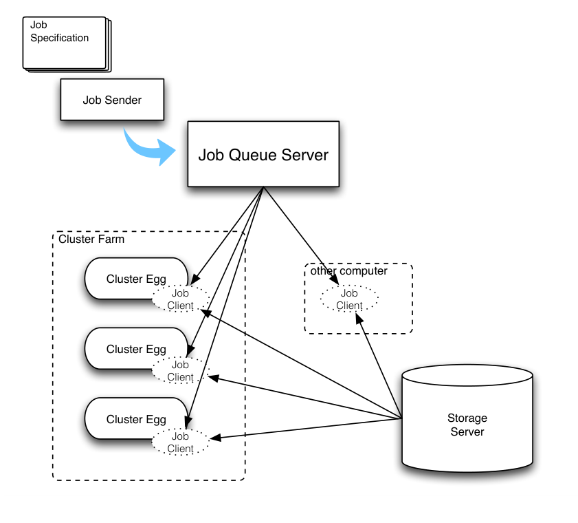

Fig. (25) shows our pipeline setup. We develop the system in haskell using Glasgow Haskell Compiler (ghc) 7.0. The job queue server is supposed to be always on and waiting for new jobs or new job requests from the client, which can run either in a cluster or on common desktops. If it runs on a cluster, a bootstrap script called clusteregg automatically installs a ready-made setup for a job client with MadGraph and the rest of the needed software. Since each job client sends its configuration when it requests a new job, the job queue server dispatches a new job for which the client is adequate (for example, if the job client does not have Mathematica, then Mathematica jobs are not assigned). A client also rechecks whether a job is doable with its current setup, and finally both parties handshake on the job assignment. After the negotiation, the job client proceeds with the job according to the job specification from the server, and the job specification and high energy physics tools are interfaced with pipeline. After the job is finished, a job client sends its results to the storage server and wipes out the temporary files. Every step of the job status is reported to the job queue server for monitoring purposes. We will announce details of the pipeline and jobqueue systems elsewhere soon.
High performance computing facilities are now practically mandatory in high energy theory projects even for understanding the implication of the current state-of-the-art high energy experiments, especially in the LHC era. Building a common computing software infrastructure adjusted to high energy physics will harness our physics community in a very positive way.
References
- [1] T. Aaltonen et. al. [ CDF Collaboration ], Combination of CDF top quark pair production cross section measurements with up to 4.6 fb-1, CDF Note No. 9913.
- [2] The CMS Collaboration, Combination of top pair production cross section in p p collisions at TeV and comparisons with theory, CMS Physics Analysis Summary CMS PAS TOP-11-001; The ATLAS Collaboration, A combined measurement of the top quark pair production cross-section using dilepton and single-lepton final states, ATLAS Note ATLAS-CONF-2011-040.
- [3] The ATLAS Collaboration, A Search for Resonances in the Lepton Plus Jets Channel using 200 pb-1 of Collisions at TeV, ATLAS Note ATLAS-CONF-2011-087
- [4] T. Aaltonen et al. [ CDF Collaboration ], First Measurement of the t anti-t Differential Cross Section in p anti-p Collisions at TeV, Phys. Rev. Lett. 102, 222003 (2009), [arXiv:0903.2850 [hep-ex]].
- [5] J. L. Hewett, J. Shelton, M. Spannowsky, T. M. P. Tait, M. Takeuchi, Meets LHC, [arXiv:1103.4618 [hep-ph]].
- [6] Y. Bai and Z. Han, Improving the Top Quark Forward-Backward Asymmetry Measurement at the LHC, arXiv:1106.5071 [hep-ph].
- [7] T. Aaltonen et al. [ CDF Collaboration ], Evidence for a Mass Dependent Forward-Backward Asymmetry in Top Quark Pair Production, Phys. Rev. D83, 112003 (2011), [arXiv:1101.0034 [hep-ex]].
- [8] J. H. Kuhn, G. Rodrigo, Charge asymmetry in hadroproduction of heavy quarks, Phys. Rev. Lett. 81, 49-52 (1998), [hep-ph/9802268].
- [9] J. H. Kuhn, G. Rodrigo, Charge asymmetry of heavy quarks at hadron colliders, Phys. Rev. D59, 054017 (1999), [hep-ph/9807420].
- [10] M. T. Bowen, S. D. Ellis, D. Rainwater, Standard model top quark asymmetry at the Fermilab Tevatron, Phys. Rev. D73, 014008 (2006), [hep-ph/0509267].
- [11] L. G. Almeida, G. F. Sterman, W. Vogelsang, Threshold Resummation for the Top Quark Charge Asymmetry, Phys. Rev. D78, 014008 (2008), [arXiv:0805.1885 [hep-ph]].
- [12] V. Ahrens, A. Ferroglia, M. Neubert, B. D. Pecjak, L. L. Yang, The top-pair forward-backward asymmetry beyond NLO, [arXiv:1106.6051 [hep-ph]].
- [13] T. Aaltonen et. al., [ CDF Collaboration ], Measurement of the Forward Backward Asymmetry in Top Pair Production in the Dilepton Decay Channel using 5.1 fb, CDF Note No. 10436.
- [14] V. M. Abazov et al. [ D0 Collaboration ], First measurement of the forward-backward charge asymmetry in top quark pair production, Phys. Rev. Lett. 100, 142002 (2008), [arXiv:0712.0851 [hep-ex]].
- [15] L. M. Sehgal, M. Wanninger, Forward - Backward Asymmetry In Two Jet Events: Signature Of Axigluons In Proton - Anti-proton Collisions, Phys. Lett. B200, 211 (1988).
- [16] J. Bagger, C. Schmidt, S. King, Axigluon Production In Hadronic Collisions, Phys. Rev. D37, 1188 (1988).
- [17] A. Djouadi, G. Moreau, F. Richard, R. K. Singh, The Forward-backward asymmetry of top quark production at the Tevatron in warped extra dimensional models, Phys. Rev. D82, 071702 (2010), [arXiv:0906.0604 [hep-ph]].
- [18] P. Ferrario, G. Rodrigo, Constraining heavy colored resonances from top-antitop quark events, Phys. Rev. D80, 051701 (2009), [arXiv:0906.5541 [hep-ph]].
- [19] P. H. Frampton, J. Shu, K. Wang, Axigluon as Possible Explanation for Forward-Backward Asymmetry, Phys. Lett. B683, 294-297 (2010), [arXiv:0911.2955 [hep-ph]].
- [20] R. S. Chivukula, E. H. Simmons, C. -P. Yuan, Axigluons cannot explain the observed top quark forward-backward asymmetry, Phys. Rev. D82, 094009 (2010), [arXiv:1007.0260 [hep-ph]].
- [21] M. Bauer, F. Goertz, U. Haisch, T. Pfoh, S. Westhoff, Top-Quark Forward-Backward Asymmetry in Randall-Sundrum Models Beyond the Leading Order, JHEP 1011, 039 (2010), [arXiv:1008.0742 [hep-ph]].
- [22] C. -H. Chen, G. Cvetic, C. S. Kim, Forward-backward asymmetry of top quark in unparticle physics, Phys. Lett. B694, 393-397 (2011), [arXiv:1009.4165 [hep-ph]].
- [23] E. Alvarez, L. Da Rold, A. Szynkman, A composite Higgs model analysis of forward-backward asymmetries in the production of tops at Tevatron and bottoms at LEP and SLC, JHEP 1105, 070 (2011), [arXiv:1011.6557 [hep-ph]].
- [24] C. Delaunay, O. Gedalia, S. J. Lee, G. Perez, E. Ponton, Extraordinary Phenomenology from Warped Flavor Triviality, [arXiv:1101.2902 [hep-ph]].
- [25] Y. Bai, J. L. Hewett, J. Kaplan, T. G. Rizzo, LHC Predictions from a Tevatron Anomaly in the Top Quark Forward-Backward Asymmetry, JHEP 1103 (2011) 003. [arXiv:1101.5203 [hep-ph]].
- [26] E. R. Barreto, Y. A. Coutinho, J. Sa Borges, Top quark forward-backward asymmetry from the model, Phys. Rev. D83, 054006 (2011), [arXiv:1103.1266 [hep-ph]].
- [27] R. Foot, Top quark forward-backward asymmetry from SU() color, Phys. Rev. D83, 114013 (2011), [arXiv:1103.1940 [hep-ph]].
- [28] A. R. Zerwekh, The Axigluon, a Four-Site Model and the Top Quark Forward-Backward Asymmetry at the Tevatron, [arXiv:1103.0956 [hep-ph]].
- [29] J. Shu, K. Wang, G. Zhu, A Revisit to Top Quark Forward-Backward Asymmetry, [arXiv:1104.0083 [hep-ph]].
- [30] U. Haisch, S. Westhoff, Massive Color-Octet Bosons: Bounds on Effects in Top-Quark Pair Production, [arXiv:1106.0529 [hep-ph]].
- [31] G. M. Tavares, M. Schmaltz, Explaining the t-tbar asymmetry with a light axigluon, [arXiv:1107.0978 [hep-ph]].
- [32] E. Alvarez, L. Da Rold, J. I. S. Vietto, A. Szynkman, Phenomenology of a light gluon resonance in top-physics at Tevatron and LHC, [arXiv:1107.1473 [hep-ph]].
- [33] R. Barcelo, A. Carmona, M. Masip, J. Santiago, Gluon excitations in t tbar production at hadron colliders, Phys. Rev. D84, 014024 (2011). [arXiv:1105.3333 [hep-ph]].
- [34] R. Barcelo, A. Carmona, M. Masip, J. Santiago, Stealth gluons at hadron colliders, [arXiv:1106.4054 [hep-ph]].
- [35] J. A. Aguilar-Saavedra, M. Perez-Victoria, Shaping the top asymmetry, [arXiv:1107.2120 [hep-ph]].
- [36] S. Jung, H. Murayama, A. Pierce, J. D. Wells, Top quark forward-backward asymmetry from new t-channel physics, Phys. Rev. D81, 015004 (2010), [arXiv:0907.4112 [hep-ph]].
- [37] K. Cheung, W. -Y. Keung, T. -C. Yuan, Top Quark Forward-Backward Asymmetry, Phys. Lett. B682, 287-290 (2009), [arXiv:0908.2589 [hep-ph]].
- [38] J. Shu, T. M. P. Tait, K. Wang, Explorations of the Top Quark Forward-Backward Asymmetry at the Tevatron, Phys. Rev. D81, 034012 (2010), [arXiv:0911.3237 [hep-ph]].
- [39] A. Arhrib, R. Benbrik, C. -H. Chen, Forward-backward asymmetry of top quark in diquark models, Phys. Rev. D82, 034034 (2010), [arXiv:0911.4875 [hep-ph]].
- [40] I. Dorsner, S. Fajfer, J. F. Kamenik, N. Kosnik, Light colored scalars from grand unification and the forward-backward asymmetry in t t-bar production, Phys. Rev. D81, 055009 (2010), [arXiv:0912.0972 [hep-ph]].
- [41] V. Barger, W. -Y. Keung, C. -T. Yu, Asymmetric Left-Right Model and the Top Pair Forward-Backward Asymmetry, Phys. Rev. D81, 113009 (2010), [arXiv:1002.1048 [hep-ph]].
- [42] B. Xiao, Y. -k. Wang, S. -h. Zhu, Forward-backward Asymmetry and Differential Cross Section of Top Quark in Flavor Violating Z’ model at , Phys. Rev. D82, 034026 (2010), [arXiv:1006.2510 [hep-ph]].
- [43] K. Cheung, T. -C. Yuan, Top Quark Forward-Backward Asymmetry in the Large Invariant Mass Region, Phys. Rev. D83, 074006 (2011), [arXiv:1101.1445 [hep-ph]].
- [44] J. Shelton, K. M. Zurek, Maximal flavor violation from new right-handed gauge bosons, Phys. Rev. D83, 091701 (2011), [arXiv:1101.5392 [hep-ph]].
- [45] E. L. Berger, Q. -H. Cao, C. -R. Chen, C. S. Li, H. Zhang, Top Quark Forward-Backward Asymmetry and Same-Sign Top Quark Pairs, Phys. Rev. Lett. 106, 201801 (2011), [arXiv:1101.5625 [hep-ph]].
- [46] B. Grinstein, A. L. Kagan, M. Trott, J. Zupan, Forward-backward asymmetry in production from flavour symmetries, Phys. Rev. Lett. 107, 012002 (2011), [arXiv:1102.3374 [hep-ph]].
- [47] K. M. Patel, P. Sharma, Forward-backward asymmetry in top quark production from light colored scalars in SO(10) model, JHEP 1104, 085 (2011). [arXiv:1102.4736 [hep-ph]].
- [48] N. Craig, C. Kilic, M. J. Strassler, LHC Charge Asymmetry as Constraint on Models for the Tevatron Top Anomaly, [arXiv:1103.2127 [hep-ph]].
- [49] Z. Ligeti, G. M. Tavares, M. Schmaltz, Explaining the t tbar forward-backward asymmetry without dijet or flavor anomalies, JHEP 1106, 109 (2011). [arXiv:1103.2757 [hep-ph]].
- [50] S. Jung, A. Pierce, J. D. Wells, Top quark asymmetry from a non-Abelian horizontal symmetry, Phys. Rev. D83, 114039 (2011), [arXiv:1103.4835 [hep-ph]].
- [51] A. E. Nelson, T. Okui, T. S. Roy, A unified, flavor symmetric explanation for the t-tbar asymmetry and Wjj excess at CDF, [arXiv:1104.2030 [hep-ph]].
- [52] M. Duraisamy, A. Rashed, A. Datta, The Top Forward Backward Asymmetry with general Z ’ couplings, [arXiv:1106.5982 [hep-ph]].
- [53] E. Gabrielli, M. Raidal, Effective axial-vector coupling of gluon as an explanation to the top quark asymmetry, [arXiv:1106.4553 [hep-ph]].
- [54] D. -W. Jung, P. Ko, J. S. Lee, S. -h. Nam, Model independent analysis of the forward-backward asymmetry of top quark production at the Tevatron, Phys. Lett. B691, 238-242 (2010), [arXiv:0912.1105 [hep-ph]].
- [55] J. Cao, Z. Heng, L. Wu, J. M. Yang, Top quark forward-backward asymmetry at the Tevatron: A Comparative study in different new physics models, Phys. Rev. D81, 014016 (2010), [arXiv:0912.1447 [hep-ph]].
- [56] Q. -H. Cao, D. McKeen, J. L. Rosner, G. Shaughnessy, C. E. M. Wagner, Forward-Backward Asymmetry of Top Quark Pair Production, Phys. Rev. D81, 114004 (2010), [arXiv:1003.3461 [hep-ph]].
- [57] D. -W. Jung, P. Ko, J. S. Lee, Longitudinal top polarization as a probe of a possible origin of forward-backward asymmetry of the top quark at the Tevatron, Phys. Lett. B701, 248-254 (2011), [arXiv:1011.5976 [hep-ph]].
- [58] D. Choudhury, R. M. Godbole, S. D. Rindani, P. Saha, Top polarization, forward-backward asymmetry and new physics, [arXiv:1012.4750 [hep-ph]].
- [59] D. -w. Jung, P. Ko, J. S. Lee, S. -h. Nam, Model-independent analysis of forward-backward asymmetry of top quark production at the Tevatron, [arXiv:1012.0102 [hep-ph]].
- [60] C. Delaunay, O. Gedalia, Y. Hochberg, G. Perez, Y. Soreq, Implications of the CDF Forward-Backward Asymmetry for Hard Top Physics, [arXiv:1103.2297 [hep-ph]].
- [61] M. I. Gresham, I. -W. Kim, K. M. Zurek, Phys. Rev. D83, 114027 (2011), [arXiv:1103.3501 [hep-ph]].
- [62] D. Krohn, T. Liu, J. Shelton, L. -T. Wang, A Polarized View of the Top Asymmetry, [arXiv:1105.3743 [hep-ph]].
- [63] M. I. Gresham, I. -W. Kim, K. M. Zurek, Searching for Top Flavor Violating Resonances, [arXiv:1102.0018 [hep-ph]].
- [64] K. Blum, C. Delaunay, O. Gedalia, Y. Hochberg, S. J. Lee, Y. Nir, G. Perez, Y. Soreq, Implications of the CDF Forward-Backward Asymmetry for Boosted Top Physics, [arXiv:1102.3133 [hep-ph]].
- [65] J. A. Aguilar-Saavedra, M. Perez-Victoria, Probing the Tevatron t tbar asymmetry at LHC, JHEP 1105, 034 (2011), [arXiv:1103.2765 [hep-ph]].
- [66] J. A. Aguilar-Saavedra, M. Perez-Victoria, Asymmetries in t production: LHC versus Tevatron, [arXiv:1105.4606 [hep-ph]].
- [67] J. M. Arnold, M. Pospelov, M. Trott, M. B. Wise, Scalar Representations and Minimal Flavor Violation, JHEP 1001, 073 (2010). [arXiv:0911.2225 [hep-ph]].
- [68] G. F. Giudice, B. Gripaios, R. Sundrum, Flavourful Production at Hadron Colliders, [arXiv:1105.3161 [hep-ph]].
- [69] B. Grinstein, A. L. Kagan, M. Trott, J. Zupan, Flavor symmetric sectors and collider physics, to appear.
- [70] J. Alwall, M. Herquet, F. Maltoni, O. Mattelaer, T. Stelzer, MadGraph 5 : Going Beyond, JHEP 1106, 128 (2011). [arXiv:1106.0522 [hep-ph]].
- [71] The ATLAS Collaboration, Observation of t-channel Single Top-Quark Production in pp Collisions at TeV with the ATLAS detector, ATLAS Note ATLAS-CONF-2011-088.
- [72] V. M. Abazov et al. [ D0 Collaboration ], Forward-backward asymmetry in top quark-antiquark production, [arXiv:1107.4995 [hep-ex]].
- [73] The ATLAS Collaboration, Measurement of the top-quark pair production cross-section in pp collisions at TeV in dilepton final states with ATLAS, ATLAS Note ATLAS-CONF-2011-100.
- [74] http://feynrules.irmp.ucl.ac.be
- [75] T. Sjostrand, P. Eden, C. Friberg, L. Lonnblad, G. Miu, S. Mrenna, E. Norrbin, High-energy physics event generation with PYTHIA 6.1, Comput. Phys. Commun. 135, 238-259 (2001). [hep-ph/0010017].
- [76] http://physics.ucdavis.edu/ conway/research/software/pgs/pgs4-general.htm
- [77] M. Cacciari, G. P. Salam, G. Soyez, The Anti-k(t) jet clustering algorithm, JHEP 0804, 063 (2008), [arXiv:0802.1189 [hep-ph]].