Spectral approximations in machine learning
Abstract
In many areas of machine learning, it becomes necessary to find the eigenvector decompositions of large matrices. We discuss two methods for reducing the computational burden of spectral decompositions: the more venerable Nyström extension and a newly introduced algorithm based on random projections. Previous work has centered on the ability to reconstruct the original matrix. We argue that a more interesting and relevant comparison is their relative performance in clustering and classification tasks using the approximate eigenvectors as features. We demonstrate that performance is task specific and depends on the rank of the approximation.
1 Introduction
Spectral Connectivity Analysis (SCA) is a burgeoning area in statistical machine learning. Beginning with principal components analysis (PCA) and Fisher discriminant analysis and continuing with locally linear embeddings [12], SCA techniques for discovering low-dimensional metric embeddings of the data have long been a part of data analysis. Moreover, newer techniques, such as Laplacian eigenmaps [2] and Hessian maps [3], similarly seek to elucidate the underlying geometry of the data by analyzing approximations to certain operators and their respective eigenfunctions.
Though the techniques are different in many respects, they share one major characteristic: the necessity for the computation of a postive definite kernel and, more importantly, its spectrum. Unfortunately, a well known speed limit exists. For a matrix , the eigenvalue decomposition can be computed no faster than . On its face, this limit constrains the applicability of SCA techniques to moderately sized problems.
Fortunately, there exist methods in numerical linear algebra for the approximate computation of the spectrum of a matrix. Two such methods are the Nyström extension [14] and another algorithm [7] we have dubbed ‘Gaussian projection’ for reasons that will become clear. Each seeks to compute the eigenvectors of a smaller matrix and then embed the remaining structure of the original matrix onto these eigenvectors. These methods are widely used in the applied SCA community e.g. [6, 5]. However, the choice as to the approximation method has remained a subjective one, largely based on the subfield of the respective researchers.
The goal of this paper is to provide a careful, comprehensive comparison of the Nyström extension and Gaussian projection methods for approximating the spectrum of the large matrices occuring in SCA techniques. As SCA is such a vast field, we concentrate on one specific technique, known as diffusion map from the graph Laplacian. In this technique, it is necessary to compute the spectrum of the Laplacian matrix . For a dataset with observations, the matrix is by , and hence the exact numerical spectrum quickly becomes impossible to compute.
Previous work on a principled comparison of the Nyström extension and Gaussian projection methods have left open some important questions. For instance, [4, 13] both provide contrasts that, while interesting, are limited in that they only consider approximation methods based on column sampling. Furthermore, performance evaluations in the literature focus on reconstructing the matrix . However, in the machine learning community, this is rarely the appropriate metric. Generally, some or all of the eigenvectors are used as an input to standard classification, regression, or clustering algorithms. Hence, there is a need for comparing the effect of these methods on the accuracy of learning machines.
We find that for these sorts of applications, neither Nyström nor Gaussian projection achieves uniformly better results. For similar computational costs, both methods perform well at manifold reconstruction. However, Gaussian projection performs relatively poorly in a related clustering task. Yet, it also outperforms Nyström on a standard classification task. We also find that the choice of tuning parameters can be easier for one method relative to the other depending on the application.
The remainder of this paper is structured as follows. In §2 we give an overview of our particular choice of SCA technique — the diffusion map from the graph Laplacian — as well as introduce both the Nyström and the Gaussian projection methods. In §3, we present our empirical results on three tasks: low dimensional manifold recovery, clustering, and classification. Lastly, §4 details areas in need of further investigation and provides a synthesis of our findings about the strengths of each approximation method.
2 Diffusion maps and spectral approximations
2.1 Diffusion map with the graph Laplacian
The technique in SCA that we consider is commonly referred to as a diffusion map from the graph Laplacian. Roughly, the idea is to construct an adjacency graph on a given data set and then find a parameterization for the data which minimizes an objective function that preserves locality. We give a brief overview here. See [10] for a more comprehensive treatment.
Specifically, suppose we have observations, . Define a graph on the data such that are the observations, is the set of connections between pairs of observations, and is a weight matrix associated with every element in , corresponding to the strength of the edge. We make the common choice (e.g. [11, §2.2.1]) of defining
| (1) |
for all such that . Further, we define a normalized version of the matrix . This can be done either symmetrically, as
| (2) |
or asymmetrically as
| (3) |
where diag. In either case, the graph Laplacian is defined to be . Here, is the by identity matrix.
One can show ([11, §8.1]) that the optimal dimensional embedding is given by the diffusion map onto eigenvectors two through of .11 1 The first eigenvalue and associated eigenvector correspond to the trivial solution and are discarded. That is, find an orthonormal matrix and diagonal matrix such that and retain the second through column of as the features. Note that we have supressed any mention of eigenvalues in the diffusion map as they only represent rescaling in our applications and hence are irrelevant to our conclusions. Also, and have the same eigenvectors.
In most machine learning scenarios, this map is created as the first step for more traditional applications. It can be used as a design (also known as a feature) matrix in classification or regression. Also, it can be used as coordinates of the data for unsupervised (clustering) techniques.
2.2 Nyström
As mentioned in §1, for most cases of interest in machine learning, is large and hence the computation of the eigenvectors of the matrix is computationally infeasible. However, the Nyström extension gives a method for computing the eigenvectors and eigenvalues of a smaller matrix, formed by column subsampling, and ‘extending’ them to the remaining columns.
The Nyström method for approximating the eigenvectors of a matrix comes from a much older technique for finding a numerical solution of integral equations. For our purposes, the Nyström method finds eigenvectors of a reduced matrix that approximates the action of .22 2 We consider the numerical spectral decomposition of the full matrix to be the ‘exact’ or ‘true’ decomposition and ignore the effects of numerical error in our nomenclature. Specifically, choose an integer and an associated index subset such that to form an matrix . Here our notation mimics common coding syntax. Subsetting a matrix with a set of indices indicates the retention of those rows or columns. Then, we find a diagonal matrix and orthonormal matrix such that
| (4) |
These eigenvectors are then extended to an approximation of the matrix by a simple formula. See Algorithm 1 for details and an outline of the procedure.
Of course, choosing the subset is important. By far the most common technique is to choose by sampling times without replacement from . We refer to this as the ‘uniform Nyström’ method. Recently, however, there has been work on making more informed and data-dependent choices. The first work in this area we are aware of can be found in [4]. More recently, [1] proposed sampling from a distribution formed by all determinants of the possible retained matrices. This is of course not feasible, and [1] provides some approximations. We use the scheme where instead of a uniform draw from , we draw from in proportion to the size of the diagonal elements in . When used, this method is referred to as the ‘weighted Nyström.’
Given an matrix and integer , compute an approximation to the eigenvectors of .
2.3 Gaussian projection
An alternate to the Nyström method is a very interesting new algorithm introduced in [7]. This new algorithm differs from other approximation techniques in that it produces, for any matrix , a subspace of col (the column space of ) through the action of on a random set of linearly independent vectors. This is in contrast to randomly selecting columns of to form a subspace of col as in [4] and the Nyström method. This is important as crucial features of col can be missed by simply subsampling columns.
2.4 Theoretical comparisons
For both the Nyström and the Gaussian projection methods, theoretical results have been developed demonstrating their performance at forming a rank approximation to . For the weighted Nyström method, [1] finds that
| (5) |
where is the approximation to via the Nyström method and is the best rank approximation. Likewise, for Gaussian projection , [7] finds that
| (6) |
where is the minimum singular value of and is a user defined tolerance for how much the projection distorts , ie:
However, these results are not generally comparable. To the best of our knowledge no lower bounds exist showing limits to the quality of the approximations formed by either method. So theoretical comparisons of these bounds are ill advised if not entirely meaningless. Furthermore, it is not clear that reconstruction of the matrix is beneficial to the machine learning tasks that the eigenvectors of are used to accomplish. SCA methods often serve as dimensionality reduction tools to create features for classification, clustering, or regression methods. This first pass dimension reduction does not obviate the need for doing feature selection with the computed approximate eigenvectors. In other words, the approximation methods help avoid one curse of dimensionality, in that large amounts of data incurrs the cost of a large amount of computations. An open question is: can the selection of the tuning parameter also avoid another curse of dimensionality in that over-parameterizing the model leads to an increase in its prediction risk?
Given an matrix and integer , we compute an orthonormal matrix that approximates col and use it to compute an approximation to the eigenvectors of , .
A major difference in the Nyström method versus the Gaussian projection method is that remains an orthonormal matrix, and hence provides an orthogonal basis for col. This can be seen by considering the output of Algorithm 2, writing as the column, and observing
| (7) |
by the orthonomality of and . This is in contrast to Algorithm 1 that produces which is a rotation of by the matrix . This difference has implications that need further exploration. However, it does show that Gaussian projection provides a numerically superior set of features with which to do learning.
3 Experimental results
In order to evaluate the approximation methods mentioned above, we focus on three related tasks: manifold reconstruction, clustering, and classification. In the first two cases, we examine simulated manifolds with and without an embedded clustering problem. For the classification task, we examine the MNIST handwritten digit database [9], using diffusion maps for feature creation and support vector machines (SVMs) to perform the classification.
3.1 Manifold recovery
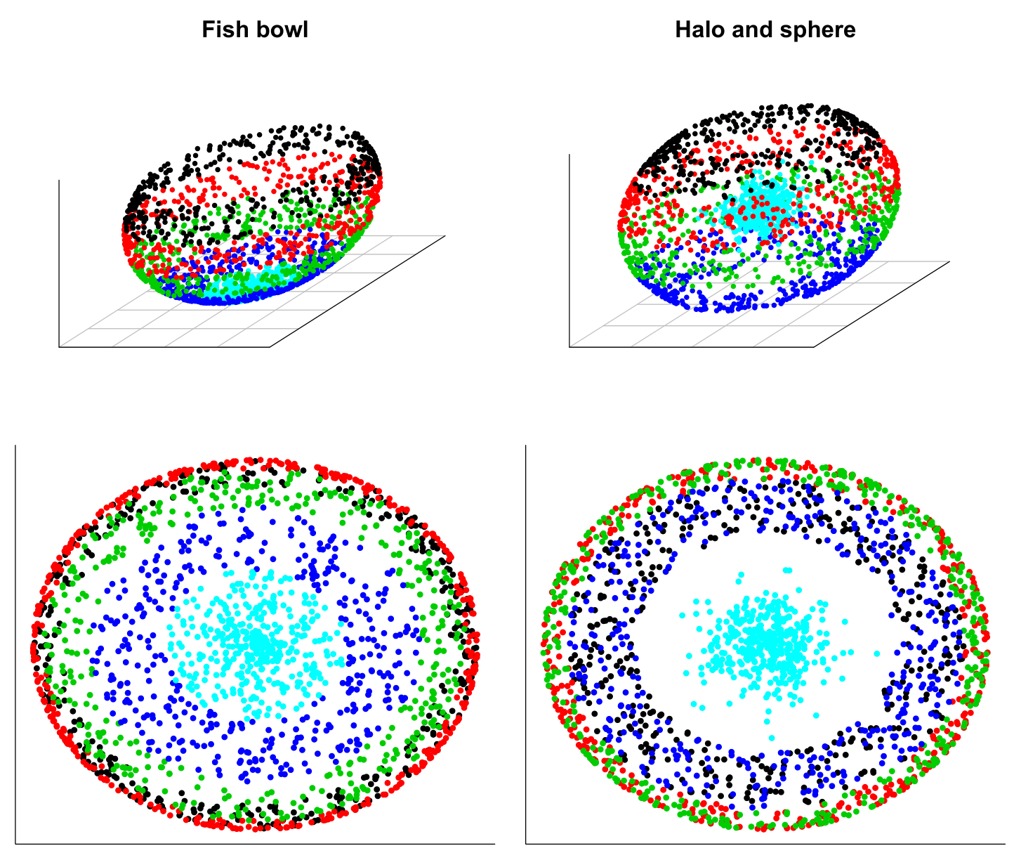
To investigate the performance of the two approximation methods through the lens of manifold recovery, we choose a standard “fishbowl” like object. It is constructed using the parametric equations for an ellipsoid:
where determine the size of the ellipsoid and determines the size of the opening. We sample uniformly over the interval, while is a regularly spaced sequence of 2000 points.
The dominant computational cost for the approximations are for Nyström and for Gaussian projection , we choose the parameter so that they have equal dominant cost. That is, if we choose for the Gaussian projection method to be a certain value, we set for the Nyström method to be . For the Nyström method, we take while for Gaussian projection, .
The manifold reconstruction of the ellipsoid is shown in Figure 2. Both methods perform reasonably well. The underlying structure is well recovered. For this figure, the tuning parameter was set at in all three cases. Changing it makes very little difference ( yields very similar figures over repeated randomizations33 3 The magnitude of the tuning parameter depends heavily on the intrinsic separation in the data). This robustness with respect to tuning parameter choice is rarely the case as we will see in the next example.44 4 Another standard manifold recovery example, the “swissroll”, is very sensitive to tuning parameter choice as well as the choice of the matrix .

3.2 Clustering
To create a clustering example similar to the manifold recovery problem, we removed the bottom fifth of the fishbowl and created a glob in the middle of the resulting halo. See Figure 1 for a plot of the shape. We consider the light blue observations in the middle one cluster and the outer ring as a second cluster. The result is a three dimensional clustering problem for which linear classifiers will fail. However, diffusion methods yield an embedding which will be separable even in one dimension via linear methods (Figure 3, first column). The next two columns show the Nyström approximation with and for Gaussian projection with . We see that Nyström provides a very faithful reproduction of the exact eigenvectors. Gaussian projection loses much of the separation present in the other two methods.
It is important to keep in mind the selection of appropriate tuning parameters. Our choice in this example is a subjective one, based on visual inspection. In this scenario, tuning parameter selection becomes very difficult, and hugely important. Small perturbations in the tuning parameter lead to poor embeddings which not only yield poor clustering solutions, but which can completely destroy the structure visible in the data alone. Furthermore, tuning parameters must be selected separately for the exact as well as the two approximate methods with no guarantee that they will be similar. In our particular parameterization, the exact reconstruction was successful for while the approximate methods required . The reconstruction via Gaussian projection shown in Figure 3 displays the best separation that we could achieve for this computational complexity. Clearly, the Nyström method performs better in this case, yielding an embedding that remains easily separable even in one dimension.
3.3 Classification
A common machine learning task is to classify data based on a labelled set of training data. When all the data (training and test) are available, using the semi-supervised approach of a diffusion map from the graph Laplacian is a very reasonable technique for providing labels for the test data. However, this technique requires a very large spectral decomposition as it is based on the entire dataset, both training and test.


We investigate classifying the handwritten digits found in the MNIST dataset and used in e.g. [9]. See the left panel of Figure 4 for fifteen randomly selected digits. Using SVM with the (approximate) eigenvectors of the graph Laplacian as features, we attempt to classify a test set using each of the above described approximation techniques. Though the digits are rotated and skewed relative to each other, we do not consider deskewing as very good classification results have been obtained using SVM without any such preprocessing (see for example [8]). We choose the smoothing parameter in the SVM via 10 fold cross-validation. Additionally, we choose the bandwidth parameter of the diffusion map, , by minimizing the misclassification error on the test set over a grid of values.
For small enough datasets, we can compute the true eigenvectors to get an idea of the efficiency loss we incurr by using each approximation. If we choose a random dataset comprised of test digits and training digits, then it is still feasible to calculate the true eigenvectors of the matrix . Table 1 displays the results with an approximation parameter of .55 5 In the manifold recovery and clustering tasks, we are essentially interested only in the first few eigenvectors of , so it makes sense to compare the two methods for equivalent computational complexity. However in the classification task, we want to create two comparable feature matrices which may then be regularized by the classifier. For this reason, it seems more natural to choose .
| Method | # Correct |
|---|---|
| 800 | |
| True eigenvectors | 756 |
| Uniform Nyström | 697 |
| Weighted Nyström | 701 |
| Gaussian projection | 725 |
We see that the Gaussian projection method has the best performance of the three considered methods. Additionally, as expected, the weighted Nyström method outperforms the uniform Nyström, but only slightly. Note that the true eigenvector misclassification rate, 5.5%, is a bit worse than that reported in [8] — 1%. We attribute this to using a much smaller training sample for our classification procedure.
Additionally, we ran a comparison with and . Here computing the true eigenvectors would begin to be truly time/resource consuming. For each we perform the grid search to minimize test set misclassification for each method. We do this a total of ten times and average the results to somewhat account for the randomness of each approximation method. The results appear on the right hand side of Figure 4. We see that again the weighted and uniform Nyström methods produce very similar misclassification rates. Interestingly, the Gaussian projection method results in a worse misclassification rate for smaller , but its performance improves markedly for larger .
4 Discussion
In this paper, we consider two main methods — the Nyström extension and another method we dub Gaussian projection — for approximating the eigenvectors of the graph Laplacian matrix . As a metric for performance, we are interested in ramifications of these approximations in practice. That is, how do the approximations affect the efficacy of standard machine learning techniques in standard machine learning tasks.
Specifically, we consider three common applications: manifold reconstruction, clustering, and classification. For the last task we additionally investigate a newer version of the Nyström method, one that allows for weighted sampling of the columns of based on the size of the diagonal elements.
We find that for these sorts of applications, neither Nyström nor Gaussian projection achieves uniformly better results. For similar computational costs, both methods perform well at manifold reconstruction, each finding the lower dimensional structure of the fishbowl as a deformed plane. However, the Gaussian projection method recovery is somewhat distorted relative to the true eigenvectors. In the clustering task, Gaussian projection performs relatively poorly. Although the inner sphere is now linearly separable from the outer ring, the embedding is much noisier than for the true eigenvectors and the Nyström extension. Lastly, we find that the weighted and uniform Nyström methods result in nearly the same misclassification rates, with perhaps a slight edge to the weighted version. But, Gaussian projection outperforms both Nyström methods as long as is moderately large: about 10% of . This value of still provides a substantial savings over computing the true eigenvectors.
References
- [1] Belabbas, M., and Wolfe, P. (2009), “Spectral methods in machine learning and new strategies for very large datasets,” Proceedings of the National Academy of Sciences, 106(2), 369–374.
- [2] Belkin, M., and Niyogi, P. (2003), “Laplacian eigenmaps for dimensionality reduction and data representation,” Neural Computation, 15(6), 1373–1396.
- [3] Donoho, D., and Grimes, C. (2003), “Hessian eigenmaps: locally linear embedding techniques for high-dimensional data,” Proceeding of the National Academy of Sciences, 100(10), 5591–5596.
- [4] Drineas, P., and Mahoney, M. (2005), “On the Nyström method for approximating a gram matrix for improved kernel-based learning for high-dimensional data,” Journal of Machine Learning Research, 6, 2153–2175.
- [5] Fowlkes, C., Belongie, S., Chung, F., and Malik, J. (2004), “Spectral grouping using the Nyström method,” IEEE Transactions on Pattern Analysis and Machine Intelligence, 26(2), 214–225.
- [6] Freeman, P., Newman, J., Lee, A., Richards, J., and Schafer, C. (2009), “Photometric redshift estimation using spectral connectivity analysis,” Monthly Notices of the Royal Astronomical Society, 398, 2012–2021, arXiv:0906.0995 [astro-ph.CO].
- [7] Halko, N., Martinsson, P. G., and Tropp, J. A. (2009), “Finding structure with randomness: Stochastic algorithms for constructing approximate matrix decompositions,” arXiv:0909.4061 [math.NA].
- [8] Lauer, F., Suen, C., and Bloch, G. (2007), “A trainable feature extractor for handwritten digit recognition,” Pattern Recognition, 40(6), 1816–1824.
- [9] LeCun, Y., Bottou, L., Bengio, Y., and Haffner, P. (1998), “Gradient-based learning applied to document recognition,” Proceedings of the IEEE, 86(11), 2278–2324.
- [10] Lee, A., and Wasserman, L. (2008a), “Spectral connectivity analysis,” Journal of the American Statistical Association, 105(491), 1241–1255.
- [11] Lee, A. B., and Wasserman, L. (2008b), “Spectral connectivity analysis,” arXiv:0811.0121 [stat.ME].
- [12] Roweis, S., and Saul, L. (2000), “Nonlinear dimensionality reduction by locally linear embedding,” Science, 106(5500), 2323–2326.
- [13] Talwalkar, A., Kumar, S., and Rowley, H. (2008), “Large-scale manifold learning,” in IEEE Conference on Computer Vision and Pattern Recognition, 2008, IEEE.
- [14] Williams, C., and Seeger, M. (2001), “Using the Nyström method to speed up kernel machines,” in Advances in Neural Information Processing Systems 13.