The Sender-Excited Secret Key Agreement Model: Capacity, Reliability and Secrecy Exponents
Abstract
We consider the secret key generation problem when sources are randomly excited by the sender and there is a noiseless public discussion channel. Our setting is thus similar to recent works on channels with action-dependent states where the channel state may be influenced by some of the parties involved. We derive single-letter expressions for the secret key capacity through a type of source emulation analysis. We also derive lower bounds on the achievable reliability and secrecy exponents, i.e., the exponential rates of decay of the probability of decoding error and of the information leakage. These exponents allow us to determine a set of strongly-achievable secret key rates. For degraded eavesdroppers the maximum strongly-achievable rate equals the secret key capacity; our exponents can also be specialized to previously known results.
In deriving our strong achievability results we introduce a coding scheme that combines wiretap coding (to excite the channel) and key extraction (to distill keys from residual randomness). The secret key capacity is naturally seen to be a combination of both source- and channel-type randomness. Through examples we illustrate a fundamental interplay between the portion of the secret key rate due to each type of randomness. We also illustrate inherent tradeoffs between the achievable reliability and secrecy exponents. Our new scheme also naturally accommodates rate limits on the public discussion. We show that under rate constraints we are able to achieve larger rates than those that can be attained through a pure source emulation strategy.
Index Terms:
Secret key capacity, Common randomness, Wiretap channel, Sender-excitation, Reliability exponent, Secrecy exponent, Degraded broadcast channel, Probing capacityI Introduction
Within the realm of information-theoretic secrecy [2], the foundations of sharing a secret key between two parties in the presence of an eavesdropper were initiated in [3, 4]. Ahlswede and Csiszár [3] studied two models: the source-type model with wiretapper (Model SW) and the channel-type model with wiretapper (Model CW). In Model SW, users obtain their observations from a discrete memoryless multiple source (DMMS), and communicate to each other via a noiseless authenticated public channel, with the objective of generating jointly held secret keys. In Model CW, one legitimate user (the sender) controls the input of a discrete memoryless broadcast channel (DMBC), sending information based upon which the legitimate receivers generate secret keys.
However, many applications cannot be exactly modeled as either a source- or a channel-type scenario. This work explores such a setting in which the sender has the ability to use a private source of randomness to excite (or influence) the “state” of the DMMS. This is similar in spirit to recent works on probing capacity and channels with action-dependent states [5, 6, 7, 8]. We derive capacity, reliability exponent, and secrecy exponent results for this setting. At one extreme, when the sender has an unlimited ability to excite the channel, and the rate of public discussion is similarly unbounded, a particular type of source emulation strategy is capacity achieving. However, when constraints are placed on the rate of public discussion we demonstrate that source emulation becomes sub-optimal. We show this through the development of a more nuanced rate-limited excitation strategy that exceeds the capacity of the emulation-based approach when subject to rate constraints [9]. Our new strategy combines a wiretap-type probing mechanism (Model CW) with a key-distillation step (Model SW) that is applied to the residual randomness. In general, we find an interplay to exist between the secrecy rate derived from the wiretapping step and the secrecy rate derived via the key-distillation step. We illustrate the tradeoff via examples. In terms of our large deviation results we show that there is a natural tradeoff between the reliability and secrecy exponents. The former generalize Gallager’s classic results in in [10, Sec. 5.6] and [11]; the latter may be specialized to Hayashi’s recent work that characterizes the rate of decay of information leakage [12] of the wiretap channels.
I-A Related Work
There are other investigations that consider non-source, non-channel models. For example, in [13, 14] users observe a DMMS and can also transmit information via a wiretap channel. However, no public discussion is allowed. The key generation scheme used is based on the observation that a public message can be transmitted via the DMBC confidentially, resulting in a higher secret key rate. In [9, 15, 16], public discussion is allowed and there may also be a helper. However, unlike our work, the sender does not also receive a sequence as part of the channel output. The sender’s ability to use both her channel output and her source of private randomness to generate the secret key is a crucial aspects of our model.
The authors in [17, 18, 19, 20, 21] considered the setting where a wiretap channel is influenced by a random state that is known by the sender (and possibly by the receiver) and thus can be treated as a correlated source. In [17, 18], the sender transmits a confidential message and the random, noncausally known, state is exploited to confuse the eavesdropper. The lower bound is proved using a combination of Gel’fand-Pinsker coding and wiretap channel coding. A similar problem but with causal state information is studied in [19] and the coding scheme involves block Markov coding, Shannon strategies, and wiretap coding. In [20, 21], the goal is to generate a secret key when the encoder (and/or decoders) have noncausal state information. The authors present a single-letter expression for the secret key capacity. The key rate consists of two parts. The first can be attributed to the rate of the confidential message sent using wiretap channel coding where the state sequence is treated as a time-sharing sequence, while a second key, independent of the first, is produced by exploiting the common knowledge of the state at the sender and the legitimate receiver.
The model considered in this paper is a generalization of the “source excitation” model of [22]. That model is motivated by the large body of work on physical-layer security (see, e.g., [23, 24]) where the unpredictable variation in the wireless channel medium serves as the source of common randomness. One approach is to sound the wireless channel using a random signal and measure the observations generated (marginalizing over the sounding signal). This “source emulation” strategy is considered in [24]. Another approach studied in [22, 23] uses deterministic sounding (no marginalization is involved). Key extraction follows by denoising the observations using a public message. Deterministic sounding requires no source of private randomness (as does source emulation), all randomness is due to the channel. The current generalization is that we now explore the source excitation model when the exciter has a source of private randomness. This allows us to exploit both random sounding (using a wiretap code) and key generation (using conditional randomness). We regard the current model as stepping stone to understanding the fundamental limits of two-way randomized channel sounding in which secrecy rate is derived from the use of two wiretap codes and from the conditional randomness produced.
I-B Main Contributions: Capacity and Error Exponents
Figure 1 shows the system considered in this paper. We can think of the terminal labeled Alice as a base station on earth equipped with a sensor. This base station transmits a random message (the selection of which is based on a private source of randomness) securely to a satellite encoder. The satellite produces sequence according to some conditional probability law. This sequence is the input to a broadcast channel (the wireless medium). The channel produces observations , and , respectively received by Alice, the legitimate user Bob, and the malicious user Eve. The goal of the two legitimate users is to generate a shared secret key – Alice based on and Bob based on , where is a public message known to all parties.
We first consider the situation in which there are no rate limits on either the public discussion () or the excitation signal (). We derive a single-letter expression for the secret key capacity of this system. The result follows through a particular kind of source emulation where (i) Alice chooses the optimum source distribution to induce (potentially subject to cost constraints on ), and (ii) Alice has the vector observation .
We then turn to the rate-limited situation and study the effect of rate limits on (i) the achievable secrecy rate, (ii) the probability of erroneous decoding at the legitimate receiver, Bob, and (iii) the key leakage rate by the eavesdropper, Eve. We focus on degraded channels and characterize the error probability in terms of a reliability exponent and the key leakage rate in terms of a secrecy exponent. In contrast to [9] where the secret key capacity of one-way key generation subject to a rate constraint is characterized, we show that the flexibility Alice has in choosing the amount of private randomness she uses in the selection of can allow a strictly higher achievable secret key rate than can be attained via pure source emulation.
We introduce a new type of decoder for the legitimate receiver, Bob, to use. This decoder is a combination of a maximum likelihood and a maximum a-posteriori (ML-MAP) decoder. Bob decodes jointly the sender’s source and the sender’s private source of randomness (or message) . The resulting reliability exponent expression can be specialized to Gallager’s channel coding error exponent [10, Sec. 5.6] and Gallager’s source coding error exponent [11]. On the other hand, in the key leakage analysis, the secrecy exponent we derive captures the leakage due to Eve’s channel and the leakage due to the correlation between Alice’s variable and Eve’s variable in a transparent manner. Our analysis builds on the work by Hayashi in [12, 25], where he links the leakage rate of a wiretap channel to channel resolvability and identification coding [26]. This connection is also examined Bloch and Laneman [27] where they derive the capacity of general wiretap channels from an information spectrum perspective [26]. Our secrecy exponent results, which are developed in Section IV, can be specialized to the wiretap channel [12, 25] and to the secret key generation from correlated source setting [28, 29, 12, 22]. The difference vis-à-vis the motivating work [22] is that the methods used to bound the exponents for both reliability and secrecy involve both wiretap channel coding and source coding. This will become clear in Section IV where we specialize our results to various known problems. Note that the criterion for exponential decay of the key leakage rate is much stronger than the usual strong secrecy [4]. We focus on this exponential notion because it quantifies how fast the error probability and information rate decays to zero and because it reveals a natural tradeoff between the attainable reliability and secrecy exponents.
I-C Paper Organization
This paper is organized as follows: In Section II, we describe the system model. We also define the secret key capacity, the capacity-reliability-secrecy region and the notion of channel degradedness. Our main results pertaining to the secret key capacity are provided in Section III. We also prove a (sometimes loose) upper bound on the secret key capacity that does not contain any auxiliary random variables, and hence is amenable to evaluation. We show that this upper bound is tight for degraded channels. We present the reliability and secrecy exponents in Section IV and connect to previous work. In Section V, we present several examples to demonstrate how the main results can be applied to channels of interest. We show the inherent tradeoff between the portions of the secret key rate due to source- and to channel-type randomness. We also show the inherent tradeoff between the reliability exponent and the secrecy exponent. The proofs of the capacity theorems and the error exponent theorems are provided in Section VI and Section VII respectively.
I-D Notation
We generally adopt the notational conventions in the book by El Gamal and Kim [30], some of which we recap here. All logarithms are to base-. Random variables are in upper case (e.g., ) and their realizations in lower case (e.g., ). The corresponding alphabets of random variables are in calligraphic font (e.g., ) and so are all sets and events (e.g., ). For vectors, and if , the abbreviation is used. In addition, . The probability mass function (pmf) of a discrete random variable is denoted as or more simply as . Random codebooks are denoted by a special script font while a codebook realization is denoted as . For an , we also commonly use the notation .
II Problem Setup
II-A The Secret Key Generation Protocol
The setting is shown in Fig. 1. Consider a 3-receiver DMBC consisting of four finite sets and a collection of conditional pmfs on . Alice, at terminal , controls the channel input sounding signal through the encoder via uses of the channel. Alice has a private source of randomness used to select an index , which influences . The legitimate receiver at terminal is known as Bob and the eavesdropper at terminal is known as Eve. There is also a noiseless public discussion channel which allows Alice to transmit a message to Bob and Eve. Let be a per-letter, bounded cost function and let be an admissible cost. A code for the secret key generation protocol consists of a tuple of functions . In particular,
- 1.
Channel Excitation: Alice selects a message uniformly at random. The (satellite) encoder sends a message-dependent input sequence ( possibly being random) satisfying
(1) The input sequence is transmitted over uses of . The output sequences , and are observed by Alice, Bob (legitimate receiver) and Eve (eavesdropper) respectively.
- 2.
One-Way (Forward) Public Discussion: After observing , Alice generates a one-way public message11 1 As in [30], we use a common notation to denote both the function as well as the output of the function . This applies in the rest of the paper. , and transmits it over a noiseless public channel.
- 3.
Key Generation: Alice generates a key . After receiving his channel output and the public message , Bob generates another key .
Note the conditional distribution of given can be factorized as . The first conditional distribution can be roughly thought of as Alice’s influence on the channel state via the sounding signal , while the second can be thought of as a state-dependent channel.
II-B Definitions
We now provide the definitions of achievable secret key rates, secret key capacity and error exponents. As a reminder, the random variables and respectively denote Alice’s and Bob’s key. The public message is denoted as .
Definition 1 (Weak Achievability).
The secret key rate is -weakly-achievable (or simply -achievable) if there exists a sequence of codes (for any pair) for the secret key generation protocol such that the following three conditions are satisfied:
| (2) | ||||
| (3) | ||||
| (4) |
Definition 2 ((Forward) Secret Key Capacity).
The secret key capacity-cost function is defined as follows:
| (5) |
We will henceforth say that is the (forward) secret key capacity (without reference to the cost ). The reliability condition in (2) implies that we would like Alice’s and Bob’s keys to agree with high probability. The secrecy condition in (3) requires that the eavesdropper cannot estimate the key given her observation and the public message . This is manifested in that the key leakage rate is arbitrarily small for sufficiently large blocklength . The rate condition in (4) implies that the entropy of should be close to . In other words the pmf of should be close to that of a uniform pmf on , so the eavesdropper can only glean a negligible amount of information.
In many practical settings, the fact that the error probability in (2) and the key leakage rate in (3) can be made arbitrarily small with increasing block length is insufficient. See Maurer’s work in [31] and a more recent exposition in [27]. It would, in fact, be desirable to quantify their rates of decay and to devise coding schemes to ensure that these decay rates are as large as possible. We formalize this by defining the notion of an achievable secret key rate-exponent triple. To simplify the exposition, in our definitions (and corresponding results) of rates with exponents, we will assume that . In other words, we do not impose a cost constraint on as in (1).
Definition 3 (Achievable Secret Key Rate-Exponent Triple).
The secret key rate-exponent triple is achievable if there exists a sequence of codes for the secret key generation protocol such that in addition to (4), the following hold:
| (6) | ||||
| (7) |
In (6), is known as the reliability exponent and in (7), is known as the secrecy exponent. Collectively, and are known as error exponents (though is not, strictly speaking, an error probability but we abuse terminology to say that both are “errors”). Definition 3 can also be interpreted as follows: If a triple is achievable, then the error probability in (2) decays22 2 Here and in the following, for a pair of positive sequences , we say that if . The notation is defined analogously. We say that if and . as and the key leakage decays as . Naturally, the constraint on the entropy of the secret key in (4) is retained in the above definition.
Definition 4 (Capacity-Reliability-Secrecy Region).
The (secret key) capacity-reliability-secrecy region is the closure of the set of achievable secret key rate-exponent triples.
In analogy to the notion of weak achievability, we can also define a more stringent notion known as strong achievability, also studied in [32, 31].
Definition 5 (Strong Achievability).
The secret key rate is strongly-achievable if is achievable for some and .
We conclude our suite of definitions by formalizing the notion of degraded channels.
Definition 6 (Degradedness).
We say that the DMBC is degraded if form a Markov chain, i.e., .
In this case, we also say that the DMBC is degraded in favor of Bob or equivalently that Eve’s observation is a degraded version of Bob’s. Note that we do not differentiate between physical and stochastic degradedness [30, Ch. 5]. The capacity results will turn out to be identical for both cases.
III Basic Capacity Results
We present our capacity results in this section. These correspond to Definitions 1 and 2 and we emphasize that and are unconstrained here. We leverage on a source emulation result by Ahlswede-Csiszár [3] to give a single-letter expression for the secret key capacity containing two auxiliary random variables taking into account that has to satisfy the cost constraint in (1). We also provide a looser upper bound that contains no auxiliary random variables. The upper bound is tight when the DMBC is degraded in favor of Bob. The capacity results in this section motivate the more refined error exponent analysis in the following section where can be constrained and we will see that a judicious choice of does not reduce in the case of degraded DMBCs.
Proposition 1 (Secret Key Capacity).
The secret key capacity of DMBC is
| (8) |
where the maximization is over all joint distributions that factor in accordance to or equivalently,
| (9) |
such that .
By repeated applications of Bayes rule, the decomposition in (9) can be written as
| (10) |
Since the DMBC is given, the optimization in (8) is over the source distribution and the auxiliary conditional distributions and . Furthermore, by using the Fenchel-Eggleston-Carathéodry Theorem [30, App. C], it can be argued that the cardinalities of the auxiliary random variables and can be bounded as and respectively.
Proof of Proposition 1.
Achievability follows from [3, Theorem 1] for Model SW with a slight modification to account for cost constraint on in (1). Fix an and a joint distribution in (9) achieving . Let be the -marginal of (9) and let its typical set33 3 The typical set defined in [30, Sec. 2.4] consists of all sequences whose type (empirical distribution) satisfies for every . The typical average lemma [30, Sec. 2.4] implies that . be . Index all the elements in as . We are only going to excite the DMBC using sequences belonging to . By the typical average lemma [30, Sec. 2.4], this ensures that for every , the almost sure cost constraint in (1) is satisfied.
The encoder has the codebook , which is known to all parties. Alice generates an index uniformly at random so in this coding scheme, for some as . Given , the encoder transmits the sequence indexed by in the codebook. Note that is arbitrarily close to one for large enough . Hence, just as in the proof of [3, Theorem 1], we can consecutively select mutually disjoint wiretap codes from (with in [3, Eq. (4.1)] replaced by , say) where each codebook contains codewords of the same type. The rest of the proof in [3, Theorem 1] follows verbatim with our in the role of there. This allows us to assert that is a one-way (forward) achievable key rate. Note that in our setting, Alice receives and also has (a function of her privately generated index ), Bob receives and Eve receives . The proof is completed by taking and using the continuity of . That is continuous follows from the continuity of , and in (9).
To find the secret key capacity for specific channels, two auxiliary random variables and solving (8) have to be identified. This may be a difficult task. In the next proposition, we provide an (albeit looser) upper bound which does not involve any auxiliary random variables. This result will turn out to be important in Section V where we present several channels for which we can calculate the secret key capacity-cost function in closed-form.
Proposition 2 (Upper Bound in Secret Key Capacity).
The secret key capacity is upper bounded as
| (11) |
where the maximization is over all input distributions such that .
The proof of this proposition is given in Section VI-B. Roughly speaking, the expression in (11) can be interpreted as the secret key capacity when Alice and Bob have full knowledge (side information) of Eve’s observation , hence the conditioning on . We note by using the techniques in Ahlswede-Csiszár [3] (and in particular Lemma 2.2 therein) that our upper bound also holds for the scenario where the parties Alice and Bob can exchange multiple messages–the multi-way discussion scenario.
In the case of degraded , the result in Proposition 2 is tight.
Corollary 3 (Secret Key Capacity of Degraded DMBCs).
If the DMBC is degraded, the secret key capacity is
| (12) |
where the maximization is over all input distributions such that .
Proof.
For the converse, we observe from Proposition 2 that the secret key capacity of the degraded DMBC can be upper bounded as
| (13) | ||||
| (14) |
The last equality is due to the fact that for degraded channels, forms a Markov chain. ∎
Notice that for a fixed , the difference of mutual informations in (12) can be decomposed into two parts:
| (15) |
where the channel and source rates are respectively defined as
| (16) | ||||
| (17) |
The first rate can be interpreted as the confidential message rate of the wiretap channel [33]. The second rate is the secret key rate from an excited correlated source previously studied in [22] for a particular sounding signal with type . In the present setup, is randomly chosen by Alice. As such, we can optimize over its distribution to find the largest “sum rate” . It turns out that there is a natural interplay and tradeoff between and . We illustrate this numerically using an example in Section V-A.
We provide an alternative proof of the capacity of degraded DMBCs via the error exponent route in the next section. We note that the flexibility of the amount of private randomness that Alice has in the form of the random message (which we did not exploit in this section) allows us to operate at a lower and yet result in a positive capacity.
IV Error Exponent Theorem
In this section, we present an inner bound for the secret key capacity-reliability-secrecy region per Definition 4. Our general result is then specialized to other known results in the literature. Recall that for the error exponent results, we consider the case when there is no cost constraint on the codewords for simplicity (i.e., ).
We make the following two observations when we employ the achievability strategy proposed in this paper which is a random binning scheme. First, the decoding error probability is only a function of marginal distribution . Second, the key leakage is only a function of marginal distribution . This means that we can characterize the achievable reliability and secrecy exponents separately as functions of each marginal distribution.
IV-A Basic Definitions
Before we present our result, we begin with a few definitions. Let
| (18) | ||||
| (19) | ||||
| (20) |
As well, define
| (21) |
Similarly, define
| (22) | ||||
| (23) |
We now define a rate-exponent region parameterized by the input distribution and the pair of auxiliary rates :
| (24) |
IV-B The Inner Bound
The following theorem provides an inner bound to the capacity-reliability-secrecy region .
Theorem 4 (Inner Bound to the Capacity-Reliability-Secrecy Region).
The union of the regions in (24) is an inner bound to the secret key capacity-reliability-secrecy region, i.e.,
| (25) |
The proof of this theorem can be found in Section VII and hinges on an ML-MAP decoding strategy. More precisely, given , Bob first uses the following rule to estimate Alice’s source of private randomness and Alice’s received sequence :
| (26) |
The function is a (random) binning function, which is defined and discussed in greater detail in Section VII-A. The exponents and represent the marginal events and , respectively. The former is a Slepian-Wolf-type exponent [11] ( to be reconstructed given vector side-information ) while the latter is a channel coding-type exponent [10, Sec. 5.6] (input and vector output ). The exponent represents the joint error event and is a hybrid of Slepian-Wolf and channel coding. Upon the decoding of , Bob declares his key to be , where is another (random) binning function. The proof for the secrecy exponent leverages on the properties of the Rényi entropy as in [12, 22].
The union of the regions in (25) is likely to be a strict inner bound since our coding scheme does not involve the use of any auxiliary random variables (unlike in Proposition 1). However, as we shall see in Section IV-D, our analysis of the ML-MAP strategy shows that all weakly-achievable rates are strongly-achievable for degraded channels.
Another reason as to why the error exponent region is likely not tight may be distilled from works by Csiszár-Narayan [15], later extended by Gohari-Anantharam [34, 35]. Consider an external agent who can recover perfectly after receiving Eve’s information and the shared secret key . If the agent were not able to recover there would be some piece of information about , independent of , that the external agent would require to know perfectly. In such a setting, Alice could reveal the needed information on the public channel without lowering the secret key rate. This follows since what would be revealed is independent of , and thus of no use to Eve. Thus, without loss of generality, we can assume the external agent knows perfectly.
Now, say that is a degraded version of . In this setting Bob can simulate . Bob also has (note that with high probability). So, Bob too can be assumed to recover perfectly. In other words, in the degraded setting there is no loss in generality in requiring Bob to recover . However, when there is a non-trivial joint distribution amongst and (i.e., the non-degraded case), it is not necessarily true that Bob can recover . Hence the error-exponent strategy may be strictly suboptimal (at least in a capacity sense for non-degraded channels). This observation is consistent with the “separation” strategy elucidated in (16) and (17) as the separation strategy–which is optimal in the degraded case–in effect implies that Bob can decode as discussed in the previous paragraph.
IV-C Positivity of Error Exponents and Interpretations
For a particular choice of input distribution , the following proposition characterizes the boundary of the achievable rate-exponent region in (24).
Proposition 5 (Positivity of Error Exponents).
The proposition can be proved by firstly verifying that (resp. ) are concave functions of (resp. ); secondly by computing the partial derivative of (resp. ) with respect to (resp. ); and finally by evaluating the slope at (resp. ). This is a standard calculation and as such, we omit the details. See [22, Theorem 3] and the accompanying remarks for similar calculations. Note that there are only two rate constraints for reliability in (27) and (28). This is because the rate constraint required for is
| (30) |
which is already implied by (28) since . Note that in the derivation of and (30), we treat as a vector output of a channel with input . We had mentioned previously that can be reduced and yet the secret-key capacity would remain unchanged if we reduce accordingly. However, we observe from (27) that there is nevertheless a lower bound on due to a marginal error event. Thus, cannot be reduced arbitrarily, and in particular not beyond the conditional entropy . Intuitively, the corner point in Fig. 2 (point ) where and may be achieved from a two-step decoding procedure where Bob first recovers through channel decoding given and then recovers via Slepian-Wolf decoding given the vector side-information ( assumed to be decoded correctly). This two-step decoding procedure is, however, not what we do in the ML-MAP decoding scheme in (26). The ML-MAP decoding scheme decodes and jointly so its exponent is likely to be higher than the two-step decoding scheme.
The first rate condition in (28) for the reliability exponent to be positive may be rewritten as follows:
| (31) |
Using (31), we see that if (i.e., the compression rate is strictly larger than the Slepian-Wolf limit as allowed by (27)), we may transmit the message reliably at rates higher than , which is the maximum transmission rate when the input distribution is used for the channel .
The rate condition in (29) for the secrecy exponent to be positive may be written in the following equivalent forms:
| (32a) | |||||
| (32b) | |||||
The authors in [22, Theorem 3] showed that the secrecy exponent is positive when . However, we observe from (32a) that if (i.e., the message rate is larger than what Eve can resolve with her channel ), the secrecy exponent is positive even though may be larger than . Similarly, observe from (32b) that if , then may be smaller than for the secrecy exponent to be positive.
IV-D Strong Achievability and Connections to Degradedness
Assume that the DMBC is degraded. We then eliminate the rates and in (28) and (29) and conclude that is strongly-achievable if
| (33) |
per (27) we also require that . The last equality holds due to the assumption of degradedness, cf. Defn. 6. See Fig. 3. This concurs with the result for the secret key capacity for degraded channels obtained using pure source emulation in Corollary 3. This alternative method of deriving the secret key capacity for the degraded case via the error exponent route demonstrates that for degraded channels, the weak and strong definitions for achievability (in Definitions 1 and 5 respectively) coincide.
IV-E Connections to Previous Results
The reliability exponent in (20) is akin to a combination of Gallager’s exponents for channel coding [10, Sec. 5.6] and for source coding with side information [11]. The secrecy exponent has been studied for the secret key agreement source model [28, 12], the corresponding channel model [12], and the source model with external deterministic excitation [22]. Hayashi [12, 25] also analyzed the exponential decay of the information leakage rate for the wiretap channel. The expression in (22) is akin to a combination of the key leakage rate due to Eve’s DMC [12] and the secrecy exponent of the excited DMMS [22].
In light of these observations, Proposition 5 may be specialized to derive conditions for the positivity of the exponents for the pure channel-type and the pure source-type models:
| Specialization | Reliability | Secrecy | |
|---|---|---|---|
| I | Channel coding | Wiretap channel | |
| [10, Theorem 5.6.2] | coding [12, Theorem 3] | ||
| II | Source coding with | Secret key generation with | |
| side information [11] | public discussion [12] | ||
| Source emulation | Source emulation | ||
| III | |||
| applied to [11] | applied to [12] |
- I.
Alice has no access to the channel output () and no public discussion (): This case specializes to the wiretap channel . In this case, the reliability exponent reduces to that of channel coding over a discrete memoryless channel (DMC) [10, Theorem 5.6.2] and (28) reduces to the condition
(34) which we recognize as the condition for reliable communication over the DMC .
In addition, our secrecy exponent reduces to Hayashi’s wiretap secrecy exponent in [12, Eq. (14)] and (33) reduces to the confidential message rate constraint
(35) which we recognize as the condition for reliable communication and secrecy for the wiretap channel. Note that the usual auxiliary random variable “” [30, Theorem 22.1] has been taken to be equal to the source in (35).
- II.
Alice has no control of the channel input: This case specializes to the secret key generation model with public discussion characterized by the DMMS studied in [4, 15, 16, 34, 35]. The reliability exponent was characterized in [11] and was stated as a special case of the main result in [22]. By letting and , (28) simplifies to
(36) which we recognize as the condition for lossless source coding of given side information [36]. This recovers an analogue of the result in [22, Theorem 3]. Inequality (36) also concurs with (27).
We remark that Watanabe et al. [29] showed that strongly secure privacy amplification is not achievable by Slepian-Wolf coding. But this does not contradict our error exponent result because the codes used in [29] have rates tending to the optimal compression rate in (36) at a rate of for some (cf. [37]). However, we operate at rates strictly above in (36) so strong secrecy is indeed possible.
- III.
Alice excites the channel with generated in an i.i.d. manner according to and considers the joint variable as her source: This is similar to the source emulation scheme adopted in the proof of Proposition 1 without cost constraint and ignoring the encoder but considering the three terminals: Alice with , Bob with , and Eve with . This is point in Fig. 2. The reliability and secrecy exponents will be of the form in [11] and [12], respectively, with i.i.d. source . Thus substituting in (28) and (29) yields
(38) (39) Upon the elimination of which, by (38), satisfies the required lower bound in (27), we have
(40) Notice that the difference of mutual informations on the RHS of (40) is for degraded DMBCs. This concurs with the secret key capacity of degraded DMBCs in Corollary 3.
As is mentioned in the Introduction, while the source emulation scheme achieves the secret key capacity, this rate cannot be strongly achieved (per Definition 5) if is upper bounded by some quantity (but nonetheless still satisfies the lower bound in (27)) if we do not also have the flexibility to concurrently set the rate of the sounding signal . Observe that the lower bound on in (38) resulting from the pure source emulation strategy (cf. the achievability proof of Proposition 1) is which is at least as large as in (27) in Proposition 5 and, in general, is strictly larger. Thus, our error exponent scheme which involves wiretap coding plus key distillation allows us to reduce from to –the difference being .
The specializations are summarized in Table I.
V Numerical Examples
We consider two examples in this section. The first example illustrates the tradeoffs involved in the capacity results in Section III. The second example illustrates the tradeoffs in the achievable error exponent results in Section IV.
V-A Capacity of the Binary On-off Channel

For our first example consider the binary on-off model
where all the variables are binary and where the operations are performed in the field of size 2. Hence, the addition above is is binary modulo-2 addition. The “channel gain” is and is .44 4 We say that a binary random variable is if . Noise is and the are mutually independent. The channel describes a model in which, in the absence of noise, Eve’s observation is strictly worse than that of Alice’s and Bob’s since is present.
If and , then Eve’s channel output is a degraded version of Bob’s. In this case, there exists a for some , with the same distribution as , and independent such that , where
Let . The first term of is
where is the binary entropy function and the operation . Similarly, the second term of can be expressed as
The secret key rate due to source can be calculated as
The second equality follows because if , the source is not observed and so there is no mutual information between and (nor between and ).
The secret key rate when the input is a source is which is plotted in Fig. 4 as a function of for the following parameters: , . Note that is a concave function of while is a linear function of . If then since are jointly statistically independent. On the other hand, if then is the all ones sequence and the is maximal since the input excites all common randomness due to the common on-off coefficient . However, when , the secrecy rate of the wiretap channel . As we decrease initially increases faster than decreases, resulting in the maximum being achieved at an intermediate value of . In this example we have observed an inherent tradeoff between the amount of the secret key rate due to common randomness and due to wiretap secrecy.
V-B Error Exponents
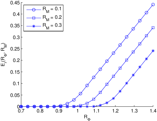
We now illustrate our error exponent results. We assume that all variables are binary valued, i.e., . We selected the parameters of the DMBC to ensure that Eve’s observation is a degraded version of Bob’s . We do so by first selecting the parameters of the conditional distribution , then we proceeded to choose the parameters in the conditional distribution . We keep the channel fixed throughout this subsection. Define the input distribution-optimized reliability exponent
| (41) |
where was defined in (21). Also define the input distribution-optimized secrecy exponent:
| (42) |
where was defined in (23). Note that for a particular set of rates , the optimal input distributions in (41) and (42) may be different. Hence, one has to use a common in (25). We append the subscript to and to allude to the fact that in the derivation of these exponents, we use both random coding [10] and random binning schemes [11].
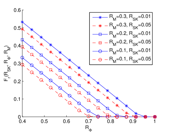
The functions and are plotted in Figs. 5 and 6 respectively. From Fig. 5, we observe that is a non-decreasing function. This is intuitive because given more information (i.e., when is large) and with fixed, Bob can decode the key with greater reliability. In contrast, is a non-increasing function. This is also intuitive because Alice’s private source of randomness is increased if is increased making it more challenging for Bob to decode the key.
From Fig. 6, we observe that is a non-increasing function. This is because as more public information is made available to Bob, with all else fixed, the key leakage rate increases, resulting in a smaller secrecy exponent. The function is non-decreasing because as Alice increases the use of her private randomness through a larger , she can conceal more of the key from Eve. Finally, is non-increasing because can be interpreted as the residual source of secrecy that can be generated by Alice and Bob while keeping Eve ignorant of the key generated.


In Fig. 7, we plot the exponents as a function of and for . The input distribution is kept fixed. Note that there is a non-empty region in the plane for which both exponents are positive, indicating that is strongly achievable. For clarity, we also present a two-dimensional visualization in Fig. 8 which helps to show the utility of our sender-excited model. We observe the following: Suppose we want to have a secret key rate of and that the public message rate must be limited to, say, due to system constraints. Then by simply adopting a source emulation strategy, (i.e., case (III) of Section IV-E), and the reliability exponent is zero even though the secrecy exponent is high. The reliability and secrecy exponents for this choice of parameters is plotted with the thick solid lines. Thus, we cannot achieve the key rate of with the fixed input distribution . However, our model affords us the flexibility to tune . If, for instance, we reduce it to while keeping we tradeoff a reduction in the secrecy exponent for an increase in the reliability exponent. With this new choice of both exponents will be positive and the key rate is (strongly) achieved with the same fixed . The exponents for this choice of parameters are plotted by the thin dashed lines.
VI Proofs of Results in Section III
VI-A Proof of Converse of Proposition 1
We start with a lemma [3, Lemma 4.1], which is a consequence of the Csiszár sum identity [30, Ch. 2].
Lemma 6.
The following equality holds for arbitrary random variables :
Proof of Converse of Proposition 1.
Fix any sequence of codes per Section II-A. Let be any -weakly achievable rate per Definition 1. Consider,
| (43) | ||||
| (44) | ||||
| (45) |
where (43) is due to Fano’s inequality ( as ), (44) is due to the secrecy condition in (3) and (45) by applying Lemma 6. Now we make the following identifications of the auxiliary random variables
| (46) |
As can be readily verified, the chosen variables and satisfy the Markov condition
as required by (9). Note that since and (random variables contained in our identifications in and in (46)) are both functions of (see Section II), by itself does not separate from and . However, the separation does hold when are grouped together by the discrete memoryless nature of the channel . Substituting the choice of auxiliary random variables in (46) into (45) yields,
Now, introduce the time-sharing random variable with uniform distribution for all and independent of . Define the random variables , , , , and . Then, we have
| (47) |
Note also that since satisfies the almost sure cost constraint in (1), holds. This implies from the definition of and that . Thus to remove the dependence on the code, we maximize (47) over all joint distributions that satisfy (9) and , i.e.,
Taking completes the proof of the converse.∎
VI-B Proof of Proposition 2
Proof.
We prove the upper bound in (11). Consider the inequalities:
| (48) | ||||
| (49) | ||||
| (50) |
where (48) follows Fano’s inequality and (49) is due to the secrecy condition (3). Continuing from (50), we have
| (51) | ||||
| (52) | ||||
| (53) |
where (51) follows because is a function of and (52) follows because the channel only depends on so .55 5 In fact, (52) holds with equality because in addition to the stated Markov relationship. Now the first term (53) can be upper bounded as follows
| (54) |
where the inequality follows by conditioning reduces entropy and the Markov chain . The second term in (53) can be written as a sum:
| (55) |
because the channel is memoryless. Substituting (54) and (55) into (53) yields
| (56) |
The proof can be completed using the time-sharing technique in the converse proof of Proposition 1. ∎
VII Proofs of Results in Section IV
In this section, we provide the proof of Theorem 4 on the capacity-reliability-secrecy region. This section will be split into three subsections: In the first subsection, we collect some relevant definitions and describe the coding scheme. The second and third subsections contain the proofs of the achievability (lower bounds) of the reliability and secrecy exponents respectively. This proves the achievability of the region defined in (24).
VII-A Definitions and Coding Scheme
We start with some definitions to describe the generation of the codewords , the key and the public message generation procedures.
Definition 7 (Random code).
A random code generated according to is a random subset of which contains length- sequences where each sequence , called a codeword, is drawn according to the pmf .
Note that we do not place any cost constraints on because we assume that in Section IV.
Definition 8 (Random binning function [11]).
A random binning function for an alphabet is a random map66 6 More precisely, is a matrix of conditional probabilities. that satisfies the following properties:
- •
Uniformity: Each element is independently and uniformly assigned to an element of .
- •
Pairwise Independence: Each pair of different is mapped , with probability for each pair of elements (not necessarily different).
- •
The random map is independent of the random code generation process as per Definition 7. More precisely,
We now introduce the notion of a random binning code for the secret key generation protocol (See Section II-A).
Definition 9 (Random binning secret key code).
A random binning secret key code is a code for the secret key generation protocol in which the public message and key are generated via two independent random binning functions:
| (57) | ||||
| (58) |
More precisely, note from (57) that is a random binning function for alphabet and from (58) that is a random binning function for alphabet .
Codebook Generation and Encoding: Fix . We use a random binning secret key code in which the codewords belong to a random code generated according to . The codewords and bin assignments are revealed to all parties before communication starts. We emphasize that by construction, this code is a code (in the sense of Section II-A with ) such that secret key rate is achievable. This is because is uniformly distributed on so (4) is satisfied.
By the definition of in (24), it suffices to show the following two assertions hold true for any :
This is what we prove in the next two subsections.
VII-B Proof for the Reliability Exponent
In this section, we will prove that is an achievable reliability exponent. Recall that Bob has access to his channel output and the public message , which was generated by Alice in accordance to the random binning function in (58). In order to analyze the error event that Bob’s key does not match Alice’s
| (59) |
we stipulate that Bob decodes both Alice’s received sequence and Alice’s source of randomness .
We restate the ML-MAP decoding rule in (26): Given , Bob declares that is the message selected by Alice and is the sequence sent to Alice if the public message bin index of agrees with , i.e.,
| (60) |
and the probabilities satisfy
| (61) |
for all other pairs such that . As mentioned previously, this is a hybrid of an ML and an MAP rule. Observe that if we were just to maximize over , this would correspond to a pure ML decoding rule for the channel as in [10, Sec. 5.6]. If instead we maximize over given is known, this would correspond to a pure MAP decoder for the source given side information as in [11].
By analyzing the ML-MAP decoder, we now upper bound the probability of event of the ensemble random binning secret key code , i.e., . Throughout, we use the notation to denote the random code (a random variable) and to denote a specific code. Define the error event that Bob decodes either or incorrectly
| (62) |
Clearly, . Thus, an upper bound for also serves as an upper bound for . Similarly, a lower bound for the exponent of is also a lower bound for the exponent of . In the interest of tractability, we upper bound [instead of ] when the ML-MAP decoder described in (60) and (61) is used. In order to bound , we decompose into the following three disjoint error events:
| (63) | |||
| (64) | |||
| (65) |
Note that the error exponent is the minimum of the exponents for , and . In the following, we only provide a detailed derivation for as it is the most interesting and unconventional. We note that for , if , (the MAP decoding part) so this analysis parallels that by Gallager for Slepian-Wolf coding [11] (reconstructing given side information and is decoded correctly). Thus, we have
| (66) |
Similarly for , we have that (Bayes rule) so this is simply the error in ML decoding for channel coding with vector output and input . Consequently, from Gallager’s book [10, Sec. 5.6],
| (67) |
Here we note that there are sounding sequences but by (60), we search within a particular bin indexed by so effectively, there are only sounding sequences explaining the leading term in (67).
Now, we analyze in detail. Consider the probability of error given that is the message sent, represents the ensemble of codewords associated to (by the random codebook construction in Definition 7), is Alice’s received sequence and is Bob’s received sequence. That is, consider
| (68) |
In the above error probability, is defined as the error event that the message , codeword and Alice’s sequence are selected in such a way that their ML-MAP objective value is higher than that of the true parameters , i.e., that and also that . Note in (68) that the error event is averaged over all incorrect codewords due to the random codebook construction (Definition 7). Now recall the assumption that the binning process is pairwise independent and also independent of the inputs (Definition 8). More precisely,
| (69) |
Let be the indicator variable of the set . By using the definition of and (69), we can upper bound the probability of as follows:
for all , where the inequality follows because for all . Let . By applying the inequality [10, pp. 136] to (68), we have
| (70) |
for any and . Now consider the error probability given message is chosen by Alice, i.e., occurs. To bound this error probability, we average over all codewords , all observed sequences and all possible sequences received by Alice , i.e.,
| (71) |
We now substitute the upper bound in (70) into (71). Pulling out from the innermost term in (70) (since it does not depend on , and ), we see that can be upper bounded as
| (72) |
where the functions and are defined as follows:
Equation (72) follows because in the line above is a dummy variable that can take on exactly values and for each , we generate codewords in the same way in the random coding construction. Now notice that if we set , then
because and in the definition of are dummy variables. As such, can be bounded as
| (73) |
where the function is defined as
Now, we recall the DMS and DMBC assumptions, i.e., that
As a result, simplifies to
and the sum in (73) can be written as a product of single-letterized terms:
| (74) |
where the function is defined as
Because each of the codewords is generated identically, each of the terms in the product in (74) is also identical. Hence,
Recall that and . In addition, note that for every . As such, taking the normalized logarithm and limit inferior of (73) yields
| (75) |
Essentially, what we have done is to develop a “hybrid” of Gallager-style error exponents for channel and lossless source coding with side information. Thus, an achievable error exponent when input distribution is used is defined in (21). The reliability exponent part of the theorem is proved for the random binning secret key code by combining the bounds for the exponents for and in (66), (67) and (75) respectively. ∎
VII-C Proof for the Secrecy Exponent
We now prove that the secrecy exponent is at least using the same coding scheme. We can use steps analogous to the proof of the direct part of Theorem 2 in [22] to obtain the following bound on the key leakage .
Lemma 7.
Define for . The key leakage can be bounded as follows:
| (76) |
for all .
The proof is provided at the end for completeness. Now we consider the inner sum in (76). By introducing the input and by repeated applications of Bayes rule,
| (77) | ||||
| (78) |
where the functions and are defined as
Equation (77) follows because form a Markov chain so and . Equation (78) follows from the uniformity of the messages in the message set , i.e., that for all . We now upper bound . This is done using the following lemma.
Lemma 8.
Let be a finite collection of non-negative numbers such that . Also, let . Then, the following inequality holds
This can be proven by noticing that is convex. We omit the details. We now make the following identifications: , and and apply Lemma 8 to . This yields the inequality
| (79) |
On account of (76), (78) and (79), we have
where the final equality follows because by the Markov chain . Now, pulling the term into the sum, we get
where the function is defined as
Now, recall that (i) the input is a DMS when averaged over all codebooks and all messages (because the generation of the codewords is done identically) and (ii) is a DMBC. Then, we have the upper bound
| (80) |
Note that the bound (80) holds for all . Recall also that , and so . Now take the normalized logarithm and limit inferior of (80) to get
The joint distribution of , namely , is induced by a particular input distribution . Essentially what we have done in this part of the proof is to develop a “hybrid” of the information leakage exponent for the wiretap channel model [12, Eq. (14)] and the excited source model [22, Theorem 3]. Hence, an achievable exponent for the key leakage given input distribution is
defined in (23).
The secrecy exponent part of the theorem is proved for the random binning secret key code.
From Random Codes to a Deterministic Code: Combining the proof in Section VII-B and proof in this section, we have shown that for the random binning secret key code, the expected probability of error decays with exponent (at least) (expectation over codebooks and random binning functions) and the expected key leakage decays exponentially with exponent (at least) . Since both are measured with respect the same (known) channel, there exists a binning secret key code that meets the ensemble behavior. More precisely, observe that , where runs through all binning secret key codes (a random code and two random binning functions) and the event is defined in (62). By Markov’s inequality,
| (81) |
Similarly, when averaged over all codes, the average key leakage is , so by Markov’s inequality,
| (82) |
From (81), by considering the complement of the event of interest, we can conclude that there exists a subset of binning secret key codes with total probability mass that exceeds (i.e., ) such that for every . Similarly, from (82) there exists a subset of binning secret key codes with total probability mass that exceeds (i.e., ) such that for every . Note that so . Thus, there exists at least one binning secret key code in the ensemble of (good) codes such that and , where the event is defined in (59). ∎
Proof of Lemma 7: Recall the assumption that the key and public message binning processes are random, uniform and independent of the random codewords (See Section VII-A for definitions and the code construction). The key leakage can be expressed as follows:
| (83) |
The conditioning is on the specific codebook used, i.e., . It remains to lower bound the conditional entropy in (83). For this purpose, let
| (84) |
be the Rényi entropy of order for . Note that . Also, by the concavity of , it can be verified that for all . Consider the conditional entropy in (83),
| (85) | ||||
| (86) |
The last inequality is due to the definition of Rényi entropy in (84) and the application of Jensen’s inequality noting that the function is convex.
Now let be a pair of random variables identically distributed to, but conditionally independent of given the events and . Recall that and are the key and public message random binning functions respectively. See (57) and (58) for definitions. Define . Then,
| (87) |
by interpreting the Rényi entropy in (84) in terms of an independent [from ] and identically distributed random variable .
Define a shorthand notation for the indicator function as
| (88) |
where and are the binning functions associated to a specific codebook . We upper bound the expectation in the logarithm in (86) on the top of the next page.
| (89) | ||||
| (90) | ||||
| (91) | ||||
| (92) | ||||
| (93) | ||||
| (94) | ||||
| (95) | ||||
| (96) | ||||
| (97) | ||||
| (98) | ||||
| (99) | ||||
| (100) | ||||
| (101) | ||||
| (102) |
The step (89) is a result of plugging (88) into the argument of the logarithm in (86). The step (90) follows by writing out the probability of a collision event in (87) explicitly as a sum. The step in (91) applies the law of total probability. We sum over all possible that are assigned bin indices for a given pair of binning function indexed by . Equation (92) follows by simple reordering of the sums.
The step (93) is an application of Jensen’s Inequality to the term in brackets since the sum over is a sum over the probability mass function (cf. (88) for the definition of this indicator function). Also, the function is concave for . We recall that , and are all fixed for this inner sum, the last being fixed by the outer expectation over . Equation (94) follows from the same reasoning as (91), i.e., the law of total probability. Equation (95) follows by simple reordering of the sums.
In (96), we used the “sifting” property of the indicator function . In (97) we split the sum over into two terms and distributed the sums over . Note that for the term, . We next applied the inequality , for to get (98).
In (99) we note that the first term is not a function of . Using the concavity of (for ), we move both the sum over and the expectation over codebooks inside the function, a step justified by Jensen’s Inequality.
In (100) we apply the uniformly random design of the binning functions. Since for every term in the sum, each of the indicator functions equals the (fixed) pair with equal probability and independently. Thus, the probability that both equal is the square (by the independence) of the reciprocal of the number of possibilities (by the uniformity), i.e., . In (101), we pulled out . Finally, we note that is a well defined (conditional) pmf and that we are missing one term in the double sum. Hence, we get (102) by upper bounding the double sum by one.
Acknowledgments
References
- [1] T.-H. Chou, V. Y. F. Tan, and S. C. Draper, “On the capacity of the sender-excited secret key agreement model,” in Proc. Allerton Conference on Communication, Control, and Computing, 2011.
- [2] Y. Liang, H. V. Poor, and S. Shamai, Information Theoretic Security. Now Publishers Inc, 2009.
- [3] R. Ahlswede and I. Csiszár, “Common randomness in information theory and cryptography part I: Secret sharing,” IEEE Trans. Inform. Theory, vol. 39, no. 4, pp. 1121–1132, 1993.
- [4] U. M. Maurer, “Secret key agreement by public discussion from common information,” IEEE Trans. Inform. Theory, vol. 39, no. 3, pp. 733–742, 1993.
- [5] T. Weissman, “Capacity of channels with action-dependent states,” IEEE Trans. Inform. Theory, vol. 56, pp. 5396–5411, Nov 2010.
- [6] H. Asnani, H. Permuter, and T. Weissman, “Probing Capacity,” IEEE Trans. Inform. Theory, vol. 57, pp. 7317–7332, Nov 2011.
- [7] K. Kittichokechai, T. J. Oechtering, M. Skoglund, and R. Thobaben, “Source and channel coding with action-dependent partially known two-sided state information,” in Proc. Int. Symp. Inform. Theory, pp. 629–633, June 2010.
- [8] H. Permuter and T. Weissman, “Source coding with a side information “vending machine”,” IEEE Trans. Inform. Theory, vol. 57, pp. 4530–4544, Jul 2011.
- [9] I. Csiszár and P. Narayan, “Common randomness and secret key generation with a helper,” IEEE Trans. Inform. Theory, vol. 46, no. 2, pp. 344–366, 2000.
- [10] R. G. Gallager, Information theory and reliable communication. New York: Wiley, 1968.
- [11] R. G. Gallager, “Source coding with side information and universal coding,” M.I.T. LIDS-P-937, 1976.
- [12] M. Hayashi, “Exponential decreasing rate of leaked information in universal random privacy amplification,” IEEE Trans. Inform. Theory, vol. 57, pp. 3989–4001, June 2011.
- [13] A. Khisti, S. Diggavi, and G. Wornell, “Secret-key generation with correlated sources and noisy channels,” in Proc. Int. Symp. Inform. Theory, pp. 1005–1009, July 2008.
- [14] V. Prabhakaran, K. Eswaran, and K. Ramchandran, “Secrecy via sources and channels – a secret key-secret message rate tradeoff region,” in Proc. Int. Symp. Inform. Theory, pp. 1010–1014, July 2008.
- [15] I. Csiszár and P. Narayan, “The secret key capacity of multiple terminals,” IEEE Trans. Inform. Theory, vol. 50, pp. 3047–3061, Dec 2004.
- [16] I. Csiszár and P. Narayan, “Secrecy capacities for multiterminal channel models,” IEEE Trans. Inform. Theory, vol. 54, pp. 2437–2452, Jun 2008.
- [17] Y. Chen and A. J. Han Vinck, “Wiretap channel with side information,” IEEE Trans. Inform. Theory, vol. 54, pp. 395–402, Jan. 2008.
- [18] W. Liu and B. Chen, “Wiretap channel with two-sided channel state information,” in Proc. Asilomar Conf. Signals, Systems and Computers, 2007, pp. 893 –897, Nov. 2007.
- [19] Y. K. Chia and A. El Gamal, “Wiretap channel with causal state information,” IEEE Trans. Inform. Theory, vol. 58, pp. 2838–2849, May 2012.
- [20] A. Khisti, S. Diggavi, and G. Wornell, “Secret key agreement using asymmetry in channel state knowledge,” in Proc. Int. Symp. Inform. Theory, pp. 2286–2290, 2009.
- [21] A. Khisti, S. Diggavi, and G. Wornell, “Secret-key agreement with channel state information at the transmitter,” IEEE Trans. on Foren. and Sec., vol. 6, pp. 672–681, Sep 2011.
- [22] T. Chou, S. C. Draper, and A. Sayeed, “Key generation using external source excitation: Capacity, reliability, and secrecy exponent,” IEEE Trans. Inform. Theory, vol. 58, pp. 2455–2474, Apr. 2012.
- [23] R. Wilson, D. Tse, and R. A. Scholtz, “Channel identification: Secret sharing using reciprocity in ultrawideband channels,” IEEE Trans. Inform. Foren. and Sec., vol. 2, pp. 364–375, Sep. 2007.
- [24] A. Agrawal, Z. Rezki, A. Khisti, and M. Alouini, “Noncoherent capacity of secret-key agreement with public discussion,” IEEE Trans. Inform. Foren. and Sec., vol. 6, pp. 565–574, Sept. 2011.
- [25] M. Hayashi, “General nonasymptotic and asymptotic formulas in channel resolvability and identification capacity and their application to the wiretap channel,” IEEE Trans. Inform. Theory, vol. 52, pp. 1562–1575, April 2006.
- [26] T. S. Han, Information-Spectrum Methods in Information Theory. Springer, 2002.
- [27] M. Bloch and J. N. Laneman, “Secrecy from Resolvability,” arXiv:1105.5419, May 2011.
- [28] C. Bennett, G. Brassard, C. Crepeau, and U. Maurer, “Generalized privacy amplification,” IEEE Trans. Inform. Theory, vol. 41, pp. 1915–1923, Nov 1995.
- [29] S. Watanabe, R. Matsumoto, and T. Uyematsu, “Strongly Secure Privacy Amplification Cannot Be Obtained by Encoder of Slepian-Wolf Code,” IEICE Transactions on Fundamentals of Electronics, Communications and Computer Sciences, vol. E93.A, no. 9, pp. 1650–1659, 2010.
- [30] A. El Gamal and Y.-H. Kim, Network Information Theory. Cambridge University Press, 2012.
- [31] U. Maurer and S. Wolf, “Information-theoretic key agreement: From weak to strong secrecy for free,” in Lecture Notes in Computer Science, pp. 351–368, Springer-Verlag, 2000.
- [32] U. M. Maurer, “The strong secret key rate of discrete random triples,” Communications and Cryptography: Two Sides of One Tapestry, pp. 271–285, Nov 1994.
- [33] A. D. Wyner, “The wire-tap channel,” The Bell Systems Technical Journal, vol. 54, pp. 1355–1387, 1975.
- [34] A. A. Gohari and V. Anantharam, “Information-theoretic key agreement of multiple terminals – I: Source model,” IEEE Trans. Inform. Theory, vol. 56, pp. 3973–3996, Aug 2008.
- [35] A. A. Gohari and V. Anantharam, “Information-Theoretic Key Agreement of Multiple Terminals–Part II: Channel Model ,” IEEE Trans. Inform. Theory, vol. 56, pp. 3997–4010, Aug. 2010.
- [36] D. Slepian and J. Wolf, “Noiseless coding of correlated sources,” IEEE Trans. Inform. Theory, vol. 19, pp. 471–480, Jul 1973.
- [37] V. Y. F. Tan and O. Kosut, “On the dispersions of three network information theory problems,” arXiv:1201.3901, Feb 2012. [Online].