NEW DEFINITION OF TMD PARTON DENSITIES
Abstract
I give an account of a new definition of transverse-momentum-dependent parton densities. The new definition solves a number of difficulties and inconsistencies in earlier definitions.
1 Introduction
In this talk, I presented a new definition of transverse-momentum-dependent (TMD) parton densities that I developed in my recent book.[1] They overcome many deficiencies of previous definitions. Numerical values for these densities with the new definition were obtained by Aybat and Rogers[2] from fits to data.
Before embarking on the QCD definition, I give a reminder about how TMD parton densities arise naturally in the parton model. Then I summarize some of the difficulties that have to be overcome in defining TMD parton densities in QCD. After that I present the new definition, compare them with other work, and indicate some of the implications of the new definition.
A number of assertions are given here without justification. For more details on the justification, see Ref. [1].
2 Basics of TMD parton densities
A motivation that TMD parton densities are useful objects to use is provided by the parton model for the Drell-Yan process, i.e., the production of a high-mass lepton pair in a high-energy hadron-hadron collision. In the parton model, the lepton pair is formed by annihilation of a quark in one hadron and an antiquark from the other, Fig. 1. This gives TMD factorization:
| (1) |
where the factors are the TMD parton densities, functions of a longitudinal momentum fraction and a transverse momentum, while is the partonic hard scattering in the lowest-order approximation. The query over the equality sign is a reminder that this is not exactly the correct TMD factorization theorem in QCD.

Because the transverse momentum of the lepton pair is the sum of the transverse momenta of the partons, the cross section (1) is directly sensitive to partonic transverse momenta. If the partons had no transverse momentum, the cross section would be a delta-function at . This contrasts with deep-inelastic scattering where only one parton participates in the hard scattering, so that its transverse momentum can be neglected with respect to the large momentum transfer in the hard scattering.
The need for TMD parton densities in Eq. (1) establishes that TMD parton densities are important quantities for a quantitative description of many hard processes.
To derive the parton model, one needs to use a cancellation of spectator-spectator interactions.[3] In addition one needs to assume other topologies of graph are unimportant, that partonic and virtuality are limited, and that no higher-order corrections are needed to the hard scattering. All of the last three assumptions are violated in QCD and are associated with a need to modify the definitions of the parton densities and the factorization formula in QCD.
2.1 Explicit definition of TMD parton density: complications in QCD
In constructing an operator definition of a TMD parton density in a hadron, I assume that the hadron is moving in the direction, and I will use light-front coordinates defined by , with , .
The parton model leads to a definition of a parton density as a hadron expectation value of the number density of a parton, as specified in light-front quantization. A first attempt at applying this in QCD uses the gauge. This is equivalent to the following gauge-invariant definition with a Wilson line in the direction11 1 Note that the derivation of factorization requires that parton densities for the Drell-Yan process use past-pointing Wilson lines.[4] :
| (2) |
where the Wilson line is
| (3) |
“F.T.” denotes a Fourier transform with respect to and , and “” denotes a transverse Wilson line at infinity. The product of Wilson lines is a path-ordered exponential of gluon fields along the line shown in Fig. 2.
There are several complications that prevent this definition from being taken literally:
- •
UV divergences. These are removed by suitable renormalization counterterms.
- •
Rapidity divergences.[5] These concern gluons whose rapidity goes to .
- •
There are Wilson line self energies. These are present in the above definition of the TMD parton density, but not in the actual cross section. They create divergences as the length of the Wilson line goes to infinity.[6]
2.2 Example: Regions for one gluon
These complications are illustrated by the graph in Fig. 3(a), where into a parton-model graph for the Drell-Yan process is inserted one gluon exchanged between the annihilating quark and antiquark. Associated with this in the factorization of collinear configurations is Fig. 3(b) for the parton density in hadron and a similar graph for the parton density in hadron .
|

| |
| (a) | (b) |

 |
 |
 |
| (a) | (b) | (c) |
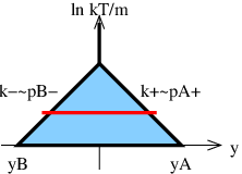
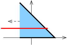
These graphs give leading power contributions from regions of gluon momentum indicated by the shaded/blue regions in Fig. 4, a plot of the space of gluon rapidity and the logarithm of its transverse momentum. A frame is used in which hadron moves in the direction and hadron in the direction. The red line indicates roughly the region needed when the transverse momentum of the lepton pair is fixed. The leading logarithm approximation is obtained by replacing the integrand in by a constant. In the cross section integrated over , the triangular region in the first plot gives the well known Sudakov double logarithm of for Fig. 3(a). The edges of the triangle are set roughly by the rapidities of the annihilating quark and antiquark, and by an infra-red cutoff on gluon . In massless perturbation theory, with , an extra doubly logarithmic contribution comes from even smaller .
Replacing the gluon and the lower part of the graph by a corresponding graph for the parton density in hadron , Fig. 3(b), gives the region shown in Fig. 4(b). The parton density graph corresponds to a good approximation for the gluon in Fig. 3(a) when it is collinear to hadron , i.e., when is sufficiently positive and is sufficiently much less than . The proof of this assertion uses a Ward identity to move the upper end of the gluon line in Fig. 3(a) onto a Wilson line.
But the approximation becomes very bad for negative , so much so, that there is a divergence in the integral to (a “rapidity divergence”).
Similarly, in Fig. 4(c), the corresponding gluonic term in the parton density in hadron reproduces the region of gluon momentum collinear to hadron , but fails badly in the positive rapidity region.
In the QCD factorization theorem that generalizes Eq. (1), these two parton-density contributions are to be added. A further problem is then that the region of central gluon rapidity is double counted.
All of the problems are overcome by finding a suitably modified definition of the TMD parton densities, together with a valid factorization theorem using the parton densities.
3 TMD factorization in QCD
TMD factorization in QCD has the general form given by Collins, Soper, and Sterman[7] (CSS):
| (4) |
Here, is a hard-scattering factor, and are TMD parton densities, and is a soft factor, with the product being a convolution in transverse momentum. Double counting subtractions are used in the definition of the factors, and there must be present some kind of cut off on rapidity divergences.
The part correctly gives the cross section when , but it fails at larger . The term corrects the errors at large ; it has the form given by ordinary collinear factorization, but with a subtraction of the low region.
All errors in Eq. (4) are suppressed by a power of . The pattern of errors in the individual terms is interesting:
| (5) |
Each of the , , and factors has a non-perturbative contribution that cannot currently be predicted from the theory; to determine the non-perturbative contributions one must fit them to data. Unfortunately, the soft factor always appears multiplied by two collinear factors (not only in the Drell-Yan process, but also in similar factorization theorems for other reactions). Thus there is no possibility of measuring independently of the parton density factors and .
A better formulation can therefore be obtained by redefining the parton density factors so that they each incorporate a square root of the soft factor. The new definition, presented below, accomplish this, albeit somewhat indirectly.
4 New definition
The new definition is in terms of unsubtracted quantities that have non-light-like Wilson lines. The unsubtracted parton density in hadron has a Wilson line of rapidity :
| (6) |
The unsubtracted soft factor has Wilson lines of rapidities and , with :
| (7) |
The definition of the TMD parton density uses an auxiliary rapidity parameter which sets the finite rapidity of certain Wilson lines. The rapidities of other Wilson lines are taken to or :
| (8) |
Here is defined to be to match a definition in Ref. [8]. A UV renormalization factor is implicit, as is the limit for the removal of the dimensional regularization of UV divergences.
The multiplications, divisions, and square roots are applied to the various factors in transverse coordinate space. They would correspond to complicated convolutions were they to be applied in transverse momentum space.
Diagrammatically, this definition can be written as
| (9) |
4.1 Why this strange definition?
This definition seems unexpectedly complicated, although the square root is to be expected given the motivation of absorbing a square root of the soft factor into each parton density in the factorization property. In fact, the definition is unique (up to the choice of the prescription for renormalization of UV divergences) given the following properties.
- •
The parton density (in transverse coordinate space) is the product of the basic parton density and powers of the soft factor.
- •
Light-like Wilson lines are used if possible:
- –
The basic parton density has only a light-like Wilson line
- –
Each soft factor has at most one non-light-like line
- –
- •
Rapidity divergences cancel, as do divergences when the length of the Wilson lines goes to infinity ().
Note that only factorization-compatible definitions should be considered, that the above definition is factorization-compatible, and that the definition implements double-counting subtractions between the soft region and the two collinear regions of momentum space.
4.2 Consequences of the strange definition
Some consequences of the new definition are:
- •
Factorization holds, as in Eq. (4), but without soft factor.
- •
Thus the TMD part of factorization is just like that in the parton model, (1), except that the parton densities depend on (and a corresponding variable for the parton density in hadron ) and on , and except that the hard scattering has higher order corrections. Note that .
- •
Rapidity divergences and Wilson-line self-energy divergences cancel.
- •
Contributions from the gauge link at infinity cancel in Feynman gauge.
- •
There is an effective cutoff on gluon rapidity at
- •
When the energy of an experiment and the dilepton mass are scaled up, the parton densities change because and increase. The dependence on these variables is governed by the dependence on , the rapidity of the non-light-like Wilson lines, and this dependence is governed by the CSS evolution equations to be discussed below.
In addition, the renormalization scale should be of order to avoid large logarithmic higher-order corrections in the hard scattering. The -dependence is governed by a renormalization-group equation.
- •
The versions of the CSS evolution equations for the newly defined parton densities are simpler than the original ones.[7] In particular, they no longer have hard-to-control power-law corrections.
5 Evolution, etc
In this section, I summarize the evolution equations and the small- expansions. These enable the TMD parton densities to be expressed in terms of (a) non-perturbative quantities without scale dependence, and (b) perturbative quantities that do not have large logarithms in the coefficients of their perturbative expansions.
The dependence of the parton density (8) on is obtained by differentiating with respect to the two soft factors that use a Wilson line of rapidity . This gives a CSS-style equation
| (10) |
The renormalization group (RG) equation of the kernel of this equation is
| (11) |
The RG equation of the TMD parton density is
| (12) |
From these equations, follows an equation for the -dependence of , and hence that
| (13) |
At small , the TMD parton density has a factorized formula in terms of ordinary integrated parton densities:
See Aybat’s talk at this conference for results at level of TMD parton densities.
6 Comparisons
In this section, I compare the new definition with some other definitions that have appeared in the literature.
6.1 CSS-style definitions
The new definition can be considered as a development of that originally proposed by Collins and Soper.[8] The old definition used the basic operator definition (2), but without a Wilson line and with the use of a non-light-like axial gauge to cut off rapidity divergences.
With this definition there was a lack of an actual proof of TMD factorization for the Drell-Yan process.[7] The problem is that Glauber region is difficult to treat in “physical gauges” such as the gauge. This lack has been remedied in Ref. [1] with the aid of the new definition. The old definition can be converted to a gauge-invariant form, with the use of non-light-like Wilson lines, which should be space-like to get factorization.[4] However there are divergences associated with self energies on the infinitely long dipolar Wilson lines. This last problem was only recently noticed, by Bacchetta, Boer, Diehl, and Mulders — see App. A of Ref. [6].
Furthermore, with the Collins-Soper definition there was a separate soft factor in the factorization formula, but as stated earlier, the non-perturbative part of the soft factor cannot be independently determined from data.
Finally the derivation of the version of the evolution equation (10) appropriate to the old definition involved ignoring errors that are power-suppressed only at small transverse momentum. Since the TMD densities are also used at large transverse momentum (in conjunction with the term in (4)), it follows that the actually-used TMD pdfs in the Collins-Soper method are not actually those that Collins and Soper defined explicitly.
Ji, Ma, and Yuan[9] improved the Collins-Soper definition of the TMD densities and the soft factor with the use of multiple non-light-like Wilson lines. However, they did not see how to take infinite-rapidity limits as in Eq. (8), which would have simplified their formalism. Their factorization formula still contains a soft factor.
6.2 Naive light-cone-gauge definition
A number of authors have defined a TMD density as the naive expectation value of a light-front parton number operator in light-cone gauge, i.e., by Eq. (2) in gauge with omission of the Wilson line. Such a definition suffers from rapidity divergences.[5] It can only be considered a valid definition if a cutoff is applied. But, as far as I can see, the need for a cutoff is often not recognized, or, if it is, a cutoff is applied in such an implicit way that it is difficult to work out what the actual definition is.
Similar problems afflict much work that uses TMD densities at small with BFKL-related approaches — see Avsar’s talk for more details.
6.3 Cherednikov and Stefanis’s work
In several recent papers, Cherednikov and Stefanis[10, 11, 12] have presented an analysis of possible definitions of TMD parton densities. They have drawn conclusions about the anomalous dimensions of the TMD parton densities and about the role of gauge links at infinity. Particular results concern the presence or absence of rapidity divergences in certain versions of light-cone-gauge quantization of QCD. Their results are based primarily on one-loop calculations. In particle, they claim that the Mandelstam-Leibbrandt prescription[13, 14] is particularly suitable, by giving finite results in situations where other methods of using the light-cone gauge give divergences.
Their gauge-invariant definition is (slightly modified from)
| (14) |
with a certain treatment of gauge links at infinity. In calculations light-cone gauge is used, with a particular cutoff in the gluon propagator:
| (15) |
where nonzero and positive. This definition in fact has uncanceled rapidity divergences from graphs that the authors appear not to calculate. Examples are
| (16) |
(Note that the regulated propagator (15) does not obey , so in these graphs the gluon attachments to the Wilson line of negative infinite rapidity are nonzero.) Furthermore Cherednikov and Stefanis do not analyze how their definition is to be used in a valid factorization formula.
6.4 Definitions in the soft-collinear effective theory (SCET) framework
In work in SCET, a number of authors have tried to make definitions of TMD functions. There are two approaches.
One is that of Becher and Neubert.[15] They use Smirnov’s subtraction methods[16] applied in a style appropriate for SCET. They are able to define the product of TMD parton densities used in the QCD TMD factorization formula, i.e., they define the product in Eq. (4). Although the product is called the product of two TMD parton densities, there are, in fact, subtractions that effectively give a soft factor. But Becher and Neubert are unable to define individual TMD parton densities. As far as I can tell, their product of TMD parton densities is the same as with my new definition; I think this is guaranteed by the use of Smirnov’s subtraction methods.
The other school in the SCET community is represented by Mantry and Petriello.[17, 18] They work with what they call an “impact parameter beam function” (iBF). Compared with the definitions such as (2) and (6), the fields in the definition of an iBF are not restricted to a null plane. So the iBFs are actually more general objects than TMD parton densities, and in some other literature would be called fully unintegrated parton densities. There are processes more exclusive than the Drell-Yan process for which their use is advantageous or even necessary. The iBFs have zero bin subtractions, which are something like the soft factors in my definition (8). However, the exact relation is not clear to me.
7 Outlook: Implications of the new definition and associated derivations
- •
We now have a precise satisfactory operator definition of TMD parton densities that can be taken literally.
- •
The gauge links at infinity are no longer needed in Feynman gauge.
- •
The definition is part of a new formalism with much better subtraction methods[1] than were previously available.
- •
- •
Hence, there is now an fully unambiguous method for calculation of the hard scattering coefficient.
- •
The formalism is much cleaner mathematically than previous versions.
- •
Although I did not explain this, there is a fully specified relation between exact and approximated parton kinematics in the hard scattering.
- •
As for future work, there is an urgent need to numerically relate TMD parton densities with the new definition to those in other formalisms.
Acknowledgments
This work was supported by the U.S. D.O.E. under grant number DE-FG02-90ER-40577. I would like to thank Ted Rogers for many useful discussions.
References
- [1] J. C. Collins. Foundations of Perturbative QCD (Cambridge University Press, Cambridge, 2011).
- [2] S. M. Aybat and T. C. Rogers, Phys.Rev., D83:114042, 2011.
- [3] J. L. Cardy and G. A. Winbow, Phys. Lett., B52:95, 1974.
- [4] J. C. Collins and A. Metz, Phys. Rev. Lett., 93:252001, 2004.
- [5] J. C. Collins, Acta Phys. Polon., B34:3103–3120, 2003.
- [6] A. Bacchetta, D. Boer, M. Diehl, and P. J. Mulders, JHEP, 08:023, 2008.
- [7] J. C. Collins, D. E. Soper, and G. Sterman, Nucl. Phys., B250:199–224, 1985.
- [8] J. C. Collins and D. E. Soper, Nucl. Phys., B194:445–492, 1982.
- [9] X.-D. Ji, J.-P. Ma, and F. Yuan, Phys. Rev., D71:034005, 2005.
- [10] I. Cherednikov and N. Stefanis, Phys.Rev., D77:094001, 2008.
- [11] I. Cherednikov and N. Stefanis, Nucl. Phys., B802:146–179, 2008.
- [12] I. O. Cherednikov and N. G. Stefanis, Phys.Rev., D80:054008, 2009.
- [13] S. Mandelstam, Nucl.Phys., B213:149–168, 1983.
- [14] G. Leibbrandt, Phys.Rev., D29:1699, 1984.
- [15] T. Becher and M. Neubert, Eur.Phys.J., C71:1665, 2011.
- [16] V. A. Smirnov, Springer Tracts Mod.Phys., 177:1–262, 2002.
- [17] S. Mantry and F. Petriello, Phys.Rev., D81:093007, 2010.
- [18] S. Mantry and F. Petriello, arXiv:1011.0757.