Alternating projections on non-tangential manifolds.
Abstract.
We consider sequences of points obtained by projecting back and forth between two manifolds and , and give conditions guaranteeing that the sequence converge to a limit . Our motivation is the study of algorithms based on finding the limit of such sequences, which have proven useful in a number of areas. The intersection is typically a set with desirable properties, but for which there is no efficient method of finding the closest point in . We prove not only that the sequence of alternating projections converges, but that the limit point is fairly close to , in a manner relative to the distance , thereby significantly improving earlier results in the field. A concrete example with applications to frequency estimation of signals is also presented.
Key words and phrases:
Alternating projections, convergence, Non-convexity2010 Mathematics Subject Classification
41A65, 49Q99, 53B251. Introduction
Let be a finite dimensional Hilbert space over and let be manifolds. Suppose that for any the closest point on , , is well defined and lets denote it by . Let the corresponding projection onto the intersection be denoted by . Suppose that we are interested in finding the closest point on and that the “projection operators” and can be efficiently computed, whereas can not. The issue treated here is how to use and to obtain an approximation of . A classical result by von Neumann [18] says that if and are affine linear manifolds, then the sequence of alternating projections
| (1.1) |
converges to . Moreover, the convergence rate is determined by the angle between and . This paper is concerned with extensions of this result to non-linear manifolds.
Hence, given , let and
| (1.2) |
In contrast to the case where is an affine linear manifold, . However, given that behave nicely, we may expect .
Alternating projection schemes of this kind have been used in a number of applications, cf. [7, 10, 12, 14, 15, 17, 16, 19]. For instance, can be the set of -matrices, and the manifolds are subsets with a certain structure, e.g. matrices with a certain rank, self-adjoint matrices, Hankel or Toeplitz matrices etc. Alternating projection schemes between several linear subsets in the infinite dimensional setting was recently investigated in [2]. Much emphasis has been put towards the usage of alternating projections for the case of complex manifolds, see for instance [3, 4]. Connections to the EM algorithm are given in [5].
In [7], Zangwill’s Global Convergence Theorem [20] is used to motivate the convergence of the alternating projection scheme above. From Zangwill’s theorem it is possible to deduce that if the sequence is bounded and the distance to is strictly decreasing, then has a convergent subsequence to a point , i.e., a result related to the fact that any bounded sequence in a compact set has a convergent subsequence. Thus, the use of Zangwill’s theorem in this context does not provide any information about whether the limit point exists, or if so, whether it is close to .
Recently, A. Lewis and J. Malick presented stronger results, valid under more restrictive conditions on and . Before discussing their results in more detail, we give two simple examples that illustrate some of the difficulties that may arise when using alternating projections on non-linear manifolds.
Example 1.1.
Let and set and . It is easily seen that and , and hence the sequence of alternating projections does not converge, cf. Figure 1. On the other hand, if , , is used as a starting point, the sequence of alternating projections will converge to .

In general, it seems reasonable to assume that if the starting point is sufficiently close to an intersection point, then the sequence does converge to a point in the intersection. The next example shows that this is not the case of limited smoothness.
Example 1.2.
Without going in to the details of the construction, we note that one can construct a -function such that, with and , the sequence of alternating projections can get stuck in projecting back and forth between the same two points. Figure 2 explains the idea.

However, if we have and , it is hard to imagine how to make a similar construction work. This is indeed impossible if we assume additional smoothness, which follows both from the present paper and [13]. In the terminology of the latter, the condition implies that and are transversal at . In general, given -manifolds and a point , we say that is transversal if
| (1.3) |
where denotes the tangent-space of at , The main result in [13] is roughly the following:
Theorem 1.3.
Let and be -manifolds and let be transversal. If is close enough to , then the sequence of alternating projections given by (1.2) converges to a point in . Moreover,
The improvement over Zangwill’s theorem is thus that the entire sequence converges, and that the assumption of boundedness no longer is necessary. Moreover, the limit is not too far off from , (although in relative terms, i.e. comparing with , it need not be particularly close either).
On the other hand, the assumption of transversalsality is rather restrictive. To demonstrate the essence of the transversality assumption, we now present two cases which are not covered by the above result, but where the conclusion still holds.
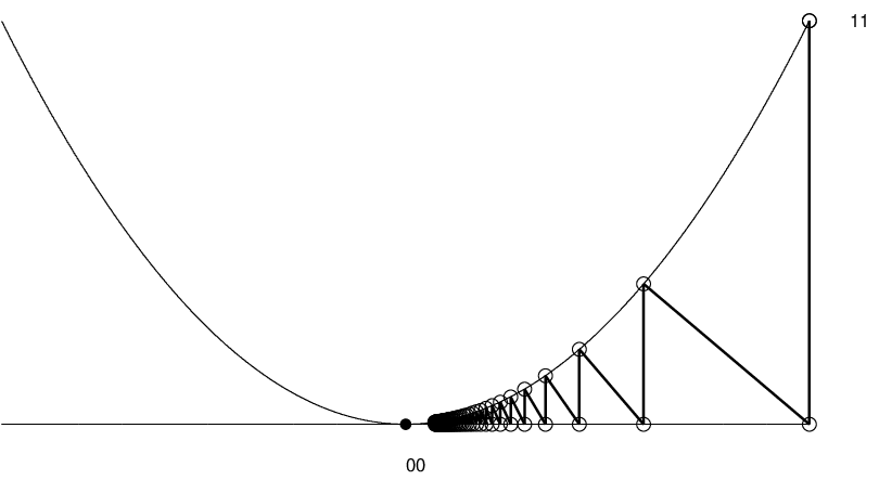
Example 1.4.
With and , transversality is not satisfied at (since ), but it is not hard to see that the sequence of alternating projections still converges to , (see Figure 3).

The difference between Example 1.2 and 1.4 is that in the latter case the manifolds are more regular.
Example 1.5.
With and and , transversality is not satisfied at , but again it seems plausible that the sequence of alternating projections converges to . See Figure 4.
In Example 1.5, the two manifolds clearly sit at a positive angle, but this situation is not covered by Theorem 1.3, since the manifolds are of too low dimension to satisfy the transversality assumption. In fact, if has dimension and has dimension , , the transversality (1.3) can never be satisfied if . But for many applications of practical interest, one has . We will introduce a concept which we call non-tangential, which loosely speaking says that the manifolds should have a positive angle in directions perpendicular to . The point in Example 1.5 is non-tangential, whereas the same point in Example 1.4 is not. A proper definition of non-tangentiality is given in Definition 4.3. A simplified version of our main result is given in what follows.
Theorem 1.6.
Given a non-tangential point there exists an such that the sequence of alternating projections (1.2) converges to a point , given that . Moreover, given any one can take such that
The full version of the main theorem is given in Section 6.
![[Uncaptioned image]](1107.4055v1/skiss.png)
The improvement over Theorem 1.3 mainly consists of two items. Primarily, the assumption that the surfaces be non-tangential is not at all restrictive, and in particular there is no implication on the dimensions of and . For the applications we are aware of, the set of tangential points is very small, if it exists at all. Secondly, as has been highlighted before, we are usually interested not just in any point of , but the closest point . Here the theorem says that in relative terms, i.e. after dividing with the distance to , the error is small if the distance to is small. It is also worth mentioning that we only assume that the manifolds are , although the manifolds are in the applications that we are aware of.
In order to motivate the need for certain technicalities in the abstract setting, as well as the need for a theorem concerning low-dimensional manifolds, we will develop the theory in parallel with an example, namely that when is the space of complex -matrices, is the set of Hankel matrices and the set of matrices of rank at most . The former is a subspace of real dimension , whereas the latter is not actually a manifold. However, it is “locally” a manifold of real dimension at all matrices with rank precisely , (which clearly constitutes the majority of matrices in the set). If is small and is a non-tangential intersection point, then , which is much less than , unless is close to . Another thing that does not match between this example and the theory outlined above is that the projection is not uniquely defined at certain points. This is common in algorithmic theory and can be dealt with by using point-to-set maps, following Zangwill [20]. However, in our case, this is not necessary since we show that the projections are locally well defined near non-tangential points, (Proposition 3.3). Moreover, from a practical perspective this is unnecessary since such points are rarely encountered in applications.
For the above example, the interest in lies in the fact that such sequences are samplings of functions which are sums of exponential functions. Given a function on an interval the alternating projections algorithm can then be used to find approximations of by sums of exponential functions, which is a problem of great practical interest. We demonstrate the idea in Figure 5. More thorough examples are conducted in [1].


2. Case study; rank matrices versus Hankel matrices
We include this section for the reader to get the picture of a typical application. However, this particular application is treated in detail in [1], and therefore we will be very brief here. In the setting considered by Lewis and Malick, the fact that is itself a manifold (around a point , say) follows by the tranversality assumption (1.3) and standard differential geometry. In our (more general) setting, may fail to be a manifold. However, in the example developed in this section, will be a manifold locally. In fact, it is not hard to see that it will always happen for algebraic manifolds, which is the case for all of the various applications presented in [7].
Let be fixed, let and let be the set of Hankel matrices, e.g., matrices of the form
| (2.1) |
is a linear subspace and, hence, a manifold at each point, of (real) dimension . Denoting the matrix in (2.1) by , where , we obtain a natural chart for , (by identifying with in the obvious way).
Given , we denote by the set of matrices of rank less than or equal to . We wish to do alternating projections as outlined in the introduction between and , which is slightly complicated by the fact that is not a manifold. However, it turns out that is locally a manifold of (real) dimension , apart from at some exceptional points. More precisely, suppose , and use the singular value decomposition of to find and unitary matrices such that
| (2.2) |
The vast majority of matrices in satisfy
| (2.3) |
and an arbitrarily small numerical perturbation will yield distinct singular values. The subset of satisfying (2.3) will be denoted , where stands for distinct. If is a manifold and its closure is such that is a union of manifolds of lower dimension than , we will say that is thin. The proof of the following proposition can be found in [1].
Proposition 2.1.
is a manifold of (real) dimension . Moreover, and is thin.
The structure of the set around the exceptional points in can be rather complicated, and although the sequence generated by the alternating projection scheme could theoretically approach such a point, we have not done any analysis of convergence properties in this setting. This seems to be a hard problem. The rate of convergence is however very poor around such points (compare Figure 1 with Figure 3). The first contains 12 iterations and the second 100.
We note that by the Eckart-Young theorem [11], it is easy to project any matrix onto its closest point in while using the Frobenius norm
Specifically, the theorem says that if is a singular value decomposition of , then the closest point in is given by replacing with where . The closest point is thus unique as long as the singular values are distinct, which is always the case when working with “real numerical” data, so we will for simplicity treat the projection onto as a well defined map which we denote by . More stringently one could work with “point to set”-maps, as in [7] and [20].
The last manifold that needs to be discussed is
i.e., the set of Hankel matrices with rank . It is easily seen that, given any , the matrix
| (2.4) |
defines a rank 1 Hankel matrix, and thus
| (2.5) |
has rank . This is the typical case, as we will show below. Let us denote the image of intersected with by , where stands for “nice”. Again, the analysis is complicated by some exceptional points. For example, is a Hankel matrix of rank which is not covered by . Moreover, rank Hankel matrices containing summands of this type are usually inside , but despite that, some investigations show that the manifold structure of collapses around such points. The sup-script is thus really more restrictive than . Nevertheless, is thin and never encountered in practice, so we omit a study of such cases. The proof of the following result can be found in [1].
Proposition 2.2.
-
is a -dimensional linear subspace.
-
is a -dimensional manifold which is dense in , its complement is thin.
-
The map is well defined on all points in except a for thin subset.
We now explain why one would like to do alternating projections between and . Let be the orthogonal projection onto , and let denote the closest point to in . Say we have a sampled function on an interval, e.g., the signal in Figure 5. Denote the corresponding sequence by and note that
| (2.6) |
We denote the weight sequence in (2.6) by and the corresponding norm on by . By Proposition 2.2, the function defining is almost surely in the range of , i.e. of the form
Such functions are precisely what one encounters when sampling sums of exponential functions, and hence is the closest such function to in the norm given by (2.6). Approximating a given function with sums of a predetermined number of exponentials is a problem with a large number of applications. There is, however, no computationally efficient method for computing . In contrast, the projections and are relatively easy to compute, and hence, by the results of this paper, we can get a fairly good approximation of by finding the limit of the sequence of alternating projections, starting at .
For the sake of efficient computations, care has to be taken concerning the implementation of and . Constructing fast algorithms for this purpose is one of the topics of a companion paper [1], where we also discuss other aspects of this specific application of alternating projections as well as give proofs of the above claims. In the present paper, we will continue discussing this application in Section 7.
3. Preliminaries
Let be a Hilbert space of dimension . Given and we write or for the open ball centered at with radius . Since is finite-dimensional it has a unique Euclidean topology. Any subset of will be given the induced topology from .
Definition 3.1.
We say that is locally an -dimensional -manifold around if there exists and a -map with the following properties:
- •
is injective for all ,
- •
- •
is a homeomorphism onto an open neighborhood of in .
This is in line with the standard definition of -manifolds, see Theorem 2.1.2 [6] for a number of equivalent definitions. As a consequence of the homeomorphism condition, note that there exists an such that
| (3.1) |
where denotes the image of . Given , there exists a unique such that . We will without further comment denote this by . All the manifolds considered in this paper are at least , and hence we have
| (3.2) |
where o stands for ‘‘little ordo’’.11 1 i.e. it stands for a function with the property that extends by continuity to 0 and takes the value 0 there. We define the tangent space by . It is a standard fact from differential geometry that this definition is independent of . Moreover, we set
i.e., is the affine linear manifold which is tangent to at . Throughout this section, will be a locally -manifold at , where and we associate with it and as in Definition 3.1 and (3.1). Moreover, there will follow a row of decreasing numbers and etc., related to the above , and the reader has to bear in mind where these numbers were defined. The following proposition basically says that the affine tangent-spaces are close to locally.
Proposition 3.2.
Let be a locally -manifold at . For each there exists , such that for all we have
- ()
- ()
Proof.
Given , we first show that is uniformly bounded above and below for . By (3.2) and the mean value theorem we have
for some on the line between and . Now, depends continuously on and its singular values depend continuously on the matrix entries [9, p191], hence
| (3.3) |
By Definition 3.1, is never zero and is compact, so both the and amount to finite positive numbers, as desired. ( denotes the closure).
We now prove ; by (3.2) and the mean value theorem we have
Since is continuous on the compact set , it is also equicontinuous. It follows that for each we can pick a such that
Set and let , , be such that implies , which we can do since is a homeomorphism with . For , we then have (by equation (3.3)) that
where , (cf equation (3.3)). By letting , the desired statement follows.
The proof of is similar. Given let be such that and note that so
Moreover, if is such that , it is easily seen that
Thus, by picking small enough we can ensure that for all , all points of the form are bounded by some pregiven . From here the proof follows a similar path as , we omit the remaining details. ∎
The value of will be determined later, so for the moment we will consider it as a constant and the corresponding value of will be kept for future use. However, was an internal variable in the above proof, and to avoid too many subindices, we let take a new value in the proof of the next proposition, (in contrast to the value of which was given in Definition 3.1 and connected to the fixed point ). The next proposition shows that projection on is a locally well defined operation.
Proposition 3.3.
Let be a locally -manifold at with . Then there exists and a map
such that for all there exists a unique closest point in which is given by . Moreover, equals if and only if .
Proof.
Recall that is the dimension of and the dimension of at . By standard differential geometry there exists an and -functions with the property that
for all , (see e.g. Theorem 2.7.7 in [6]). Define via
Consider the set of points whose multiplicity under is greater than 1, (i.e. all points hit more than once by ). By the inverse function theorem, the set can not have 0 as an accumulation-point, for it says that there exists an such that restricted to is a diffeomorphism onto its image. Pick and pick such that
| (3.4) |
and
| (3.5) |
Note that, given there exists a unique such that and moreover by (3.5). We define
To see that is a -map, let be given by and note that
We now show that have the desired properties. By the construction,
Now suppose is a closest point to . Since we clearly must have so by (3.4) there exists a with . Since we know that is completely determined by in the vicinity of . In particular, it makes sense to talk about and it is easily seen that , for by (3.2) we have
and hence the scalar product needs to be zero for all ’s. Thus there is a such that . But since is the unique point with this property, we deduce that and hence . This establishes the first part of the proposition. Now let be as in the second part of the proposition. As above we have with and the orthogonality implies that there exists a with and again this implies , as desired. ∎
4. Non-tangentiality
Suppose now that we are given closed sets and which locally are manifolds around an intersection point .
Definition 4.1.
An intersection point will be called regular if there are numbers , and such that
- •
is locally an -dimensional -manifold at ,
- •
is locally an -dimensional -manifold at .
Note that the set of regular points is clearly a relatively open set in . Next, we introduce angles. For more information on angles, we refer to [13].
Definition 4.2.
For any regular point , we define the angle of and at to be the of the number
Given a linear subspace we let denote the orthogonal projection onto . It is easily verified that
| (4.1) | ||||
If and are hyperplanes through the origin, then it is clear that the above definition coincides with the classical definition;
| (4.2) |
However, it is important to note that and are not necessarily the same. For example, take and . Then and is a regular point. Moreover whereas . What goes wrong above is clearly that the two surfaces are tangential to each other in the direction , and it is intuitively clear that when this is not the case, the two concepts should coincide. To avoid such obstacles, we therefore introduce:
Definition 4.3.
and are said to be non-tangential at if is regular and they have a positive angle at , i.e. if . We will often simply say that is non-tangential.
Note that the angle is always a number between 0 and , so in an intuitive sense only exceptional points do not satisfy non-tangentiality. We have no intention of formalizing this statement, but point out already that for the example considered in Section 2, this is indeed the case, which will be proven in [1].
Theorem 4.4.
With the notation as in Section 2, we have that the set of tangential points between and is thin in .
In the general setting, pathological examples do exist. For example, take and . However, when and are defined by polynomials, one can use similar methods, as in the proof of Theorem 4.4, to show that under mild conditions, if non-tangentiality holds at one point, then it holds everywhere except for a thin set. We will not pursue this.
By (4.1) it is easy to see that is non-tangential if and only if
| (4.3) |
which in turn happens if and only if
| (4.4) |
This latter condition is usually referred to as clean intersection in microlocal analysis. We have chosen the terminology non-tangential since it is more intuitive. We now show that non-tangentiality is a weaker concept than transversality, defined in (1.3).
Proposition 4.5.
Let and be two -manifolds and a transversal point. A transversal point is also non-tangential.
Proof.
Applying the implicit function theorem to easily yields that is a -manifold of dimension at . Thus has dimension and has dimension . Thus
But by transversality the sum of the above subspaces equals , which can only happen if (4.3) is satisfied. ∎
We will denote by , and the objects from Section 3 associated to , and , e.g. , by , and respectively. We thus omit subindex when dealing with . We now prove that for non-tangential points, the angle as defined here and the classical angle of the respective tangent spaces coincide.
Proposition 4.6.
If is non-tangential, then
Proof.
Proposition 4.7.
The function in Definition 4.2 is (on the set of regular points in ). In particular, non-tangentiality is a local property, i.e. if is non-tangential, then the same holds for all in a neighborhood of .
Proof.
Let be a regular point and let be the usual chart. We need to show that is around 0. By standard differential geometry (see e.g. [6]) there exists -functions defined on the domain of such that
It is easy to see that (with or )
| (4.5) |
Since the dimension of is constant , it is easy to see that the functions on the right are as well. Moreover, as the dimension of the space on the left in (4.5) is constant , we can pick of the functions on the right and put them as columns of an injective matrix such that
for in a neighborhood of 0. By we have for around 0 that
| (4.6) |
(Note that this is not true with the classical definition when the two ranges have a non-trivial intersection, but with the definition here it works.) Moreover, it is easy to see that
where has been omitted for readability. Combining this with (4.6) and the fact that singular values are -functions of the matrix entries, it is clear that is near , as desired. ∎
5. Properties of the projection operators
Let , , etc. be as before, i.e., -manifolds with a non-tangential intersection point . We assume that and continue to use the convention of denoting objects related to the -manifold without subindex. In Propositions 3.2 and 3.3 the quantities and appears. These are not necessarily the same and they depend on an auxiliary constant originating from Proposition 3.2. In this section we let be a fixed number (which we will determine later), and we let denote the minimum of all possible ’s from Section 3 related to the 3 manifolds. The above will not be repeated in the statements of the results below. Thus, we can apply any result from Section 3 to either of the manifolds considered here. Moreover, letting denote either or nothing, we let be such that
and such that the results of Section 3 applies to each with . We also assume that .

Given an affine linear manifold , we denote by the orthogonal projection onto . We introduce maps , ( or ), via
Thus, resemble but is slightly different. projects onto whereas projects onto the tangent plane of taken at the closest point to in , i.e. , (see Fig 6). A proper estimate of the difference is given in Proposition 5.2.
Lemma 5.1.
The operators and are -maps in . Moreover, we can select a number such that the image of under , as well as any composition of two of those maps, is contained in .
Proof.
The second part is an immediate consequence of the continuity of the maps. Let denote or and set . Note that is a -map in by Proposition 3.3 and the choice of . Moreover,
from which the result follows. ∎
Proposition 5.2.
Given any and or , we have
Proof.
By Lemma 5.1 we have that Proposition 3.2 applies to the point . It is no restriction to assume that , which we now do. Denote , and , (see Fig. 6). Let and be elements of and such that , and note that
We thus have to show that
| (5.1) |
First note that by Proposition 3.2 () there exists a point in . Thus
and hence is a member of the set
| (5.2) |
However, by Proposition 3.2 () we have that also is a member of
| (5.3) |
The left hand side of (5.1) is thus dominated by the supremum of the function
subject to the conditions in (5.2) and (5.3). Either by geometrical considerations or the method of Lagrange multipliers, it is not hard to deduce that this supremum is attained for and of the form and where . We now have a two-dimensional problem of circles and cones, and in the remainder of the proof we treat and as elements of . Given in the intersection of (5.2) and (5.3), it is easily seen (see Fig. 7) that
since this is the height of the cone at the outer edge of the circle. The problem becomes simpler if we replace the cone in (5.3) by the following strip:
| (5.4) |

From Figure 7, and some freshman formulas, it is readily verified that the sought supremum is dominated by where is the angle given by
Since we have assumed that , the proposition thus follows if we establish that
By dividing with at suitable places, one sees that this is equivalent to
Using and we obtain
since the function on the right clearly is bounded, and a few calculations show that the maximum is attained at which gives as an upper bound. ∎
Lemma 5.3.
Given we have
Proof.
Lemma 5.4.
Let and be given. If satisfies and , then
Proof.
If we are done, otherwise
which easily gives the desired estimate. ∎
The next result will be the main tool for proving convergence of the alternating projections.
Theorem 5.5.
Let be a non-tangential point and assume that and are -manifolds. Then for each and each there exists a positive such that for all we have
- ()
- ()
Moreover the same holds true with the roles of and reversed.
Proof.
Fix such that and pick an such that
| (5.5) |
which we can do since is continuous by Proposition 4.7. Let be such that By Lemma 5.1 and Proposition 3.3, and are -functions, and hence we can pick such that
| (5.6) |
for all , (recall that was chosen in the beginning of this section). Finally, we fix such that
| (5.7) |
This may seem like a circle argument, because and depends on which depends on via , and the ’s appears in (5.7). However, this is easily circumvented by first choosing with , say, and pick values of , , . Then, once the real has been chosen via (5.7) we can redefine and accordingly without violating (5.5) or (5.6).
![[Uncaptioned image]](1107.4055v1/skiss2.png)
Now, pick an such that
and let . We begin with proving . Denote and and note that so . There is no restriction to assume that , which we do from now on. We thus need to show that . Put and . (See Figure 5 and recall the by Lemma 5.3). First, note that by Proposition 5.2
| (5.8) |
and moreover by (5.6) and Proposition 5.2 we have that
| (5.9) | ||||
By Lemma 5.3 we have so part () follows by (5.6), (5.7), (5.9) and the calculation
We turn to part (). Clearly and by Lemma 5.3 we also have Thus
| (5.10) |
whereas () amounts to showing that . Recall (5.9) and apply Lemma 5.4 with , , and . We see that either
| (5.11) |
or , in which case we are done since the constant is less than by (5.7). We thus assume that (5.11) holds. Note that
| (5.12) |
by (5.8). Combining (5.10), (5.11) and (5.12) we get
by (5.7). ∎
6. Alternating projections
We are finally ready for the main theorem. The third conclusion below was not mentioned in the introduction. It basically says that if the angle between and is not too close to 0, the sequence of alternating projections will converge within machine precision within a fairly low number of iterations. In the terminology of [8], converges “R-linearly” with rate less than . For example, if , then we will hit single precision () at , since single precision has 24 bits of significant precision.
Theorem 6.1.
Let be locally non-tangential -manifolds around , and let and be given. Then there exists an such that the sequence of alternating projections
- ()
converges to a point
- ()
- ()
Proof.
Let and in Theorem 5.5 be given by and
| (6.1) |
Let be given by Theorem 5.5 and pick
| (6.2) |
such that , (recall that , by assumption). The latter condition ensures that
| (6.3) |
Let and note that
| (6.4) |
First note that and that by Lemma 5.3, so
Applying Theorem 5.5 we get
as long as
| (6.5) |
Assuming this for the moment we get
| (6.6) |
and (Theorem 5.5 and Lemma 5.3)
| (6.7) |
The sequence is thus a Cauchy sequence, and hence converges to some point . By (6.6) the sequence must also converge, and the limit point is again , which thus satisfies since is continuous. By the triangle inequality, the fact , (6.1) and (6.7) we have
and combining this with (6.3), (6.4), (6.6) we also have
where the last inequality follows by (6.2). With these estimates at hand, it is easy to turn the above argument into a proper induction proof in which (6.5) is verified at each step. We omit the details. ∎
7. Rank matrices versus Hankel matrices; numerical examples
We now continue the example in Section 2 and the application to approximation of a signal by sums of exponential functions, as outlined towards the end. By Theorem 4.4, an arbitrary intersection point of and is almost surely non-tangential. Given the signal we let be the closest “sum of exponentials” to in the -norm, see (2.6). Theorem 6.1 thus says that if is not too large, the sequence of alternating projections will converge to an , where is a sum of exponentials. More precisely, let
Then for every there exists an such that if , then
We now discuss what happens if is not close enough to that Theorem 6.1 can be applied for any . Since both and are contractions, the sequence of alternating projections (with ) will be bounded. Thus it has a convergent subsequence, and the limit point is easily seen to be in . It is not hard to deduce that as . The only way the whole sequence could avoid converging is thus if it switches endlessly along the valleys of the thin set of tangential points, thereby avoiding the surrounding hills made by the open sets , where is given by Theorem 6.1 (with say) for all non-tangential ’s, and for the thin set of tangential ’s. That this could happen seems highly unlikely to us, and we have certainly never encountered it in practice. However, we leave it as an open problem to prove that this can not occur.
For practical purposes, it is of course of interest that be a relatively large number, (given some fixed and ). Inspecting the proof Theorem 6.1, one gets the impression that will not be distinguishable even with binoculars. To test the actual relationship between and in Theorem 6.1, (with ), we conducted a few experiments which we now present. A function22 2 In this section we will sloppily say function when we talk of its sampling, i.e. a sequence. is written as a sum of exponential functions, and then is generated by adding a smaller function to . is normalized such that , (recall (2.6)), is chosen such that is orthogonal to at , (with respect to the Hilbert-Schmidt norm). By Proposition 3.3, is likely very close to , and so we will estimate by and by . Note that there is no explicit way to compute . We set
Let be a parameter taking values and . For each value of we randomly generate 50 normalized ’s as above, and for each we randomly generate a with . The supremum of should give us an idea of what value of allows for such an as in Theorem 6.1. The results are demonstrated in Figure 8 and Figure 9. The difference between the two is that Figure 8 used white noise, and in Figure 9, the “noise” consisted of sums of randomly generated exponentials. Judging from these figures, seems to be a good rule of thumb, although this will of course vary substantially from one application to another. The method seems to work slightly better for the case of white noise.


8. Summary and open problems
We have developed a theoretical framework that enables us to understand convergence properties of alternating projection schemes. This provides substantially stronger results than previously available, e.g., for theorems relying solely on Zangwill’s Global Convergence Theorem, which neither provide convergence rate estimates nor information about how far away the computed approximation is from the optimal value. Moreover, in contrast to the theory developed for the case of transversal manifolds, our framework provides more information under very non-restrictive requirements on the manifolds.
We end by noting a few open problems. We first discuss smoothness. By examples similar to Example 1.2, it is not hard to see that one needs the manifolds to be at least for the alternating projections to converge. By inspection of the proofs, one easily sees that for Theorem 6.1 to hold, it suffices with , i.e. that is Lipschitz continuous. It is thus an open question whether Theorem 6.1 is true assuming only . Next we discuss non-tangentiality. Again, Example 1.2 can be tailored such that the alternating projections does not converge, despite assuming , if we allow the manifolds to be tangential. However, for all applications we are aware of, the manifolds are algebraic, and it seems quite unlikely that a similar thing could happen in this case. We conjecture that for algebraic manifolds, the sequence of alternating projections will always converge, without any additional assumptions. Recall Example 1.4, where the sequence clearly converges albeit extremely slowly. For practical purposes, non-tangentiality is thus still vital.
9. Acknowledgements
This work was supported by the Swedish Research Council and the Swedish Foundation for International Cooperation in Research and Higher Education.
Acknowledgement: This work was partially conducted at Lund University, supported by the Swedish Research Council; Grant 2008-23883-61232-34
References
- [1] Fredrik Andersson, Marcus Carlsson, and Per Anders Ivert, A fast alternating projection method for complex frequency estimation., Submitted.
- [2] Catalin Badea, Sophie Grivaux, and Vladimir Müller, A generalization of the Friedrichs angle and the method of alternating projections, Comptes Rendus Mathematique 348 (2010), no. 1-2, 53 – 56.
- [3] H. H. Bauschke and J. M. Borwein, On the convergence of von Neumann’s alternating projection algorithm for two sets, Set-Valued Analysis 1 (1993), 185–212.
- [4] Heinz H. Bauschke and Jonathan M. Borwein, On projection algorithms for solving convex feasibility problems, SIAM Rev. 38 (1996), 367–426.
- [5] Heinz H. Bauschke, Dominikus Noll, Anna Celler, and Jonathan M. Borwein, An em algorithm for dynamic spect, IEEE TRANS. MED. IMAG 18 (1999), no. 3.
- [6] M. Berger and B. Gostiaux, Differential geometry: Manifolds, curves and surfaces., Springer Verlag, 1988.
- [7] J.A. Cadzow, Signal enhancement-a composite property mapping algorithm, Acoustics, Speech and Signal Processing, IEEE Transactions on 36 (1988), no. 1, 49 –62.
- [8] J. E. Dennis and R.B. Schnabel, Numerical methods for unconstrained optimization and nonlinear equations., Prentice-Hall, New Jersey, 1983.
- [9] J. N. Franklin, Matrix theory., Dover Publications in Mineola, N.Y., 2000.
- [10] K.M. Grigoriadis, A.E. Frazho, and R.E. Skelton, Application of alternating convex projection methods for computation of positive toeplitz matrices, Signal Processing, IEEE Transactions on 42 (1994), no. 7, 1873 –1875.
- [11] Roger A. Horn and Charles R. Johnson, Topics in matrix analysis, Cambridge University Press, Cambridge, 1994. MR 1288752 (95c:15001)
- [12] Aharon Levi and Henry Stark, Signal restoration from phase by projections onto convex sets, J. Opt. Soc. Am. 73 (1983), no. 6, 810–822.
- [13] Adrian S. Lewis and Jérôme Malick, Alternating projections on manifolds, Math. Oper. Res. 33 (2008).
- [14] Ye Li, K.J.R. Liu, and J. Razavilar, A parameter estimation scheme for damped sinusoidal signals based on low-rank hankel approximation, Signal Processing, IEEE Transactions on 45 (1997), no. 2, 481 –486.
- [15] Biao Lu, Dong Wei, B.L. Evans, and A.C. Bovik, Improved matrix pencil methods, Signals, Systems Computers, 1998. Conference Record of the Thirty-Second Asilomar Conference on, vol. 2, nov 1998, pp. 1433 –1437 vol.2.
- [16] Ivan Markovsky, Structured low-rank approximation and its applications, Automatica 44 (2008), 891–909.
- [17] Robert J. Marks, II, Alternating projections onto convex sets, pp. 476–501, Academic Press, Inc., Orlando, FL, USA, 1996.
- [18] John Von Neumann, Functional operators, volume ii: The geometry of orthogonal spaces, Princeton University Press, 1950.
- [19] V.U. Prabhu and D. Jalihal, An improved ESPRIT based time-of-arrival estimation algorithm for vehicular OFDM systems, Vehicular Technology Conference, 2009. VTC Spring 2009. IEEE 69th, april 2009, pp. 1 –4.
- [20] W. I. Zangwill, Nonlinear programming, Prentice Hall, Englewood Cliffs, N. J., 1969.