At the $1/M$ order, the most general Higgs superpotential reads [16]

$$W=\mu\hat{H}_{u}\hat{H}_{d}+\frac{\omega}{2M}\left(\hat{H}_{u}\hat{H}_{d}\right)^{2}~,$$

(1)

where $\hat{H}_{u}$ and $\hat{H}_{d}$ are the Higgs superfields with hypercharge $+1/2$ and $-1/2$, respectively and we denote $\hat{H}_{u}\hat{H}_{d}\equiv\hat{H}_{u}^{+}\hat{H}_{d}^{-}-\hat{H}_{u}^{0}\hat{H}_{d}^{0}$. The dimensionless parameter $\omega$ is taken to be of order 1 and complex.

In addition to the $1/M$ suppressed term in the superpotential, a corresponding SUSY breaking term is added to the Lagrangian [16],

$$\mathcal{L}\supset\alpha\frac{\omega m_{S}}{2M}(H_{u}H_{d})^{2}~,$$

(2)

where $\alpha$ is another free parameter of order 1 and complex. The scale $m_{S}$ is the scale of the SUSY breaking terms of the physics beyond the MSSM and therefore $m_{S}\ll M$ is necessary to integrate out the complete SUSY multiplets of the new degrees of freedom at a common scale M. The scale $m_{S}$ can be connected to the scale of the soft SUSY breaking terms of the MSSM (i.e. the sfermion and gaugino masses), but it is possible to allow for sizable differences between these scales. To ensure validity of the effective description of the BMSSM physics in terms of higher dimensional operators, $m_{S}$ (as well as $\mu$) has to be sufficiently small compared to $M$, for $\alpha$ and $\omega$ of O(1).

At the renormalizable level, the resulting tree level scalar potential then reads

	$\displaystyle V_{\rm{ren}}$	$\displaystyle=$	$\displaystyle V_{\rm{MSSM}}+\left(\alpha\frac{\omega m_{S}}{2M}(H_{u}H_{d})^{2}-\frac{\omega\mu^{*}}{M}(H_{u}H_{d})(H_{u}^{\dagger}H_{u}+H_{d}^{\dagger}H_{d})~+~h.c.\right)$		(3)
		$\displaystyle=$	$\displaystyle(m_{H_{u}}^{2}+|\mu|^{2})H_{u}^{\dagger}H_{u}+(m_{H_{d}}^{2}+|\mu|^{2})H_{d}^{\dagger}H_{d}+\left(B\mu(H_{u}H_{d})+h.c.\right)$
			$\displaystyle+\frac{g_{2}^{2}}{8c_{W}}(H_{d}^{\dagger}H_{d})^{2}+\frac{g_{2}^{2}}{8c_{W}}(H_{u}^{\dagger}H_{u})^{2}-\frac{g_{2}^{2}}{4c_{W}}(H_{d}^{\dagger}H_{d})(H_{u}^{\dagger}H_{u})+\frac{g_{2}^{2}}{2}(H_{u}^{\dagger}H_{d})(H_{d}^{\dagger}H_{u})$
			$\displaystyle+\left(\alpha\frac{\omega m_{S}}{2M}(H_{u}H_{d})^{2}-\frac{\omega\mu^{*}}{M}(H_{u}H_{d})(H_{u}^{\dagger}H_{u}+H_{d}^{\dagger}H_{d})~+~h.c.\right)~,$

and for later convenience we define

$$\lambda_{5}=|\lambda_{5}|e^{i\phi_{5}}\equiv\frac{\alpha\omega m_{S}}{M}~,~~~\lambda_{6}=|\lambda_{6}|e^{i\phi_{6}}\equiv\frac{\omega\mu^{*}}{M}~.$$

(4)

The $1/M$ operator in the superpotential leads to two additional non-renormalizable dimension six terms

$$V_{6}=\frac{\lambda_{8}}{M^{2}}(H_{u}H_{d})(H_{u}^{\dagger}H_{d}^{\dagger})(H_{u}^{\dagger}H_{u})+\frac{\lambda_{8}^{\prime}}{M^{2}}(H_{u}H_{d})(H_{u}^{\dagger}H_{d}^{\dagger})(H_{d}^{\dagger}H_{d})~,$$

(5)

with $\lambda_{8}=\lambda_{8}^{\prime}=|\omega|^{2}$. These terms are essential to stabilize the Supersymmetric electro-weak Symmetry Breaking (sEWSB) vacuae analyzed in [22]. Thanks to these non-renor-malizable terms, the potential is automatically bounded from below.

At the $1/M^{2}$ order, there can be additional operators in the Kähler potential that modify the quartic couplings of the Higgs potential. Their possible impact has been analyzed in [19, 20]. In this work instead, we focus on the leading effects generated by the $1/M$ operators in (1) and (2). While additional $1/M^{2}$ operators can lead to an additional increase of the lightest Higgs mass, we do not expect them to change our main conclusions.

The three parameters $B\mu$, $\alpha$ and $\omega$ can in general be complex. We follow the usual convention adopted in studies of the MSSM and absorb the phase of $B\mu$ by a rephasing of the two Higgs doublets. In addition, we will assume all possible complex parameters of the MSSM (e.g. gaugino masses, $\mu$ parameter etc.) to be real. If these parameters were complex, CP violating effects in the Higgs sector would be possible at the 1-loop level and would add to the tree level effects. In this work we consider the phases of $\alpha$ and $\omega$ as the only Beyond the Standard Model sources of CP violation.

We parametrize the Higgs fields as¹¹ 1 Here we neglect the possibility of charge breaking vevs. As shown in [23] this is a good approximation in regions of parameter space that lead to a stable vacuum.

$$H_{u}=e^{i\theta_{u}}\begin{pmatrix}H_{u}^{+}\\ \frac{1}{\sqrt{2}}(v_{u}+h_{u}+ia_{u})\end{pmatrix}~,~~~H_{d}=e^{i\theta_{d}}\begin{pmatrix}\frac{1}{\sqrt{2}}(v_{d}+h_{d}+ia_{d})\\ H_{d}^{-}\end{pmatrix}~,$$

(6)

where $v_{u}=v\sin\beta=vs_{\beta}$ and $v_{d}=v\cos\beta=vc_{\beta}$ with $v=246$ GeV are the two vacuum expectation values (VEVs) and $\tan\beta=t_{\beta}=v_{u}/v_{d}$ is their ratio.

While the relative phase of the Higgs fields $\theta_{u}-\theta_{d}$ can be rotated away by a $U(1)_{Y}$ transformation, $\theta\equiv\theta_{u}+\theta_{d}$ is a physical phase. Therefore, the following three extremal point conditions have to be satisfied at the minimum of the potential

$$\frac{\partial V}{\partial{\rm Re}H_{u}}=\frac{\partial V}{\partial{\rm Re}H_{d}}=\frac{\partial V}{\partial\theta}=0~.$$

(7)

Using the first two conditions in Eq. (7), the two soft masses $m_{H_{u}}$ and $m_{H_{d}}$ can be traded for $v$ and $\tan\beta$. The third condition determines the phase of the Higgs VEV, $\theta$, as a function of the phases of $\alpha$ and $\omega$ and reads

$$v^{2}c_{\beta}s_{\beta}|\lambda_{5}|\sin(\phi_{5}+2\theta)+v^{2}|\lambda_{6}|\sin(\phi_{6}+\theta)-2B\mu\sin\theta=0~.$$

(8)

Contrary to the MSSM, the BMSSM predicts in general already at tree level a non-zero phase of the Higgs fields at the minimum. In Sec. 3, we will show that constraints coming from Electric Dipole Moments (EDMs) imply that the phase of the VEV is typically rather small $\theta\lesssim O(0.1)$.

To ensure that the stationary point of the potential defined by (7) is a minimum, the corresponding Hessian has to be positive definite. However, the conditions to have a stationary point and the requirement on the Hessian do not necessarily lead to a unique solution. If the quartic couplings along the D-flat direction are negative, then a second minimum in the $v_{u}-v_{d}$ plane may arise for large field values that is stabilized by the $1/M^{2}$ suppressed terms in (5). If this second minimum is deeper, the physical minimum at $v=246$ GeV is unstable and will decay into the second deeper minimum. In Fig. 1 we show in the $\mu-m_{S}$ plane the region that is allowed by the requirement of absolute vacuum stability. The criterion of absolute stability particularly leads to stringent upper bounds on the value of the $\mu$ parameter. In accordance with the findings of [23], we observe that the portion of allowed parameter space shrinks for smaller values of the charged Higgs mass. This behavior with $M_{H^{\pm}}$ holds, varying the value of the NP scale $M$ or the two phases of $\omega$ and $\alpha$, even if their value can have a rather sizable impact on the allowed values for $\mu$. Combining the requirement of vacuum stability with the bound on the mass of the chargino, that leads to a lower bound on the absolute value of $\mu$ of $\sim 100$ GeV, the allowed regions for $\mu$ are strongly constrained, especially for low values of the charged Higgs mass (see the blue contours in Fig. 1 corresponding to $M_{H^{\pm}}=150$ GeV).

However, one should keep in mind that the requirement of absolute vacuum stability is rather conservative: it would be sufficient to impose that the EW vacuum is metastable, provided that its life time is longer than the age of the universe. This possibility has been discussed in [23] in the context of the BMSSM without CP violation. Using simple analytic approximations for the bounce action [36], we checked that the viable parameter space indeed opens up to some extent if we allow for a metastable vacuum. However, to be conservative, we require always absolute stability of the vacuum in the discussion of the Higgs phenomenology.

We now briefly review the effects of the higher dimensional operators introduced in the previous section and in particular of the new physics phases on the Higgs spectrum. In order to keep a clear comparison to the case without CP violation, we write the mass matrices of the neutral Higgs bosons in the basis that would diagonalize it in absence of new sources of CP violation

$$\begin{pmatrix}h\\ H\end{pmatrix}=\begin{pmatrix}c_{\alpha}&-s_{\alpha}\\ s_{\alpha}&c_{\alpha}\end{pmatrix}\begin{pmatrix}h_{u}\\ h_{d}\end{pmatrix}~,~~~\begin{pmatrix}G\\ A\end{pmatrix}=\begin{pmatrix}s_{\beta}&-c_{\beta}\\ c_{\beta}&s_{\beta}\end{pmatrix}\begin{pmatrix}a_{u}\\ a_{d}\end{pmatrix}~.$$

(9)

The angle $\alpha$ is given by

	$\displaystyle\sin 2\alpha$	$\displaystyle=$	$\displaystyle-\frac{M_{A}^{2}+M_{Z}^{2}}{M_{H}^{2}-M_{h}^{2}}\sin 2\beta+\frac{2v^{2}|\lambda_{6}|\cos(\phi_{6}+2\theta)}{M_{H}^{2}-M_{h}^{2}}~,$		(10)
	$\displaystyle\cos 2\alpha$	$\displaystyle=$	$\displaystyle-\frac{M_{A}^{2}-M_{Z}^{2}}{M_{H}^{2}-M_{h}^{2}}\cos 2\beta-\frac{v^{2}|\lambda_{5}|\cos(\phi_{5}+2\theta)}{M_{H}^{2}-M_{h}^{2}}\cos 2\beta~.$		(11)

In absence of CP violation, $M_{A}$ is the mass of the pseudoscalar Higgs²² 2 In the CP violating scenario we are studying, $M_{A}$ as well as $M_{h}$ and $M_{H}$ are only auxiliary parameters and not physical masses.

$$M_{A}^{2}s_{\beta}c_{\beta}=B\mu\cos\theta-\frac{v^{2}}{2}|\lambda_{6}|\cos(\phi_{6}+\theta)-v^{2}|\lambda_{5}|s_{\beta}c_{\beta}\cos(\phi_{5}+2\theta)~,$$

(12)

and $M_{h}^{2}$ and $M_{H}^{2}$ are the masses of the two scalars, namely the eigenvalues of the mass matrix

	$\displaystyle M_{S}^{2}$	$\displaystyle=$	$\displaystyle M_{A}^{2}\begin{pmatrix}c_{\beta}^{2}&-c_{\beta}s_{\beta}\\ -c_{\beta}s_{\beta}&s_{\beta}^{2}\end{pmatrix}+M_{Z}^{2}\begin{pmatrix}s_{\beta}^{2}&-c_{\beta}s_{\beta}\\ -c_{\beta}s_{\beta}&c_{\beta}^{2}\end{pmatrix}$		(13)
			$\displaystyle+v^{2}|\lambda_{6}|\cos(\phi_{6}+\theta)\begin{pmatrix}2c_{\beta}s_{\beta}&1\\ 1&2c_{\beta}s_{\beta}\end{pmatrix}+v^{2}|\lambda_{5}|\cos(\phi_{5}+2\theta)\begin{pmatrix}c_{\beta}^{2}&0\\ 0&s_{\beta}^{2}\end{pmatrix}~.$

While the Goldstone boson $G$ is not affected by the presence of CP violation, the 3 physical Higgs bosons mix in presence of CP violating phases. In the basis $(h,H,A)$, their mass matrix can be written as

$$\mathcal{M}_{H}^{2}=\begin{pmatrix}M_{h}^{2}&0&M_{hA}^{2}\\ 0&M_{H}^{2}&M_{HA}^{2}\\ M_{hA}^{2}&M_{HA}^{2}&M_{A}^{2}\end{pmatrix}~,$$

(14)

where the mixing terms are given by

	$\displaystyle M_{hA}^{2}$	$\displaystyle=$	$\displaystyle-\frac{v^{2}}{2}\left(c_{\beta+\alpha}|\lambda_{5}|\sin(\phi_{5}+2\theta)-2s_{\beta-\alpha}|\lambda_{6}|\sin(\phi_{6}+\theta)\right)~,$		(15)
	$\displaystyle M_{HA}^{2}$	$\displaystyle=$	$\displaystyle-\frac{v^{2}}{2}\left(s_{\beta+\alpha}|\lambda_{5}|\sin(\phi_{5}+2\theta)-2c_{\beta-\alpha}|\lambda_{6}|\sin(\phi_{6}+\theta)\right)~.$		(16)

The Higgs mass matrix (14) can be diagonalized by an orthogonal matrix $O$

$$O^{T}\mathcal{M}_{H}^{2}O={\rm diag}(M_{H_{1}}^{2},M_{H_{2}}^{2},M_{H_{3}}^{2})~,$$

(17)

where $M_{H_{i}}^{2}$ are the three eigenvalues.

In order to get an analytical understanding of the dependence of the Higgs spectrum of the model on the several phases, we give approximate expressions for the masses in the decoupling limit $M_{A}\gg M_{Z}$, performing a simultaneous expansion in $1/\tan\beta$ and $1/M$

	$\displaystyle M_{H_{1}}^{2}$	$\displaystyle\simeq$	$\displaystyle M_{Z}^{2}+\frac{4v^{2}}{\tan\beta}|\lambda_{6}|\cos(\phi_{6}+\theta)+\frac{v^{4}}{M_{A}^{2}}|\lambda_{6}|^{2}\cos^{2}(\phi_{6}+\theta)$		(18)
			$\displaystyle+\frac{3}{2\pi^{2}}\frac{m_{t}^{4}}{v^{2}}\left[\log\left(\frac{\tilde{m}_{t}^{2}}{m_{t}^{2}}\right)+\frac{|A_{t}|^{2}}{\tilde{m}_{t}^{2}}-\frac{|A_{t}|^{4}}{6\tilde{m}_{t}^{4}}\right]~,$
	$\displaystyle M_{H_{2}}^{2}$	$\displaystyle\simeq$	$\displaystyle M_{A}^{2}+\frac{v^{2}}{2}|\lambda_{5}|\Big(\cos(\phi_{5}+2\theta)-1\Big)~,$		(19)
	$\displaystyle M_{H_{3}}^{2}$	$\displaystyle\simeq$	$\displaystyle M_{A}^{2}+\frac{v^{2}}{2}|\lambda_{5}|\Big(\cos(\phi_{5}+2\theta)+1\Big)~.$		(20)

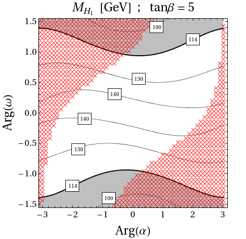
In the second line of (18) we also included the dominant 1-loop corrections to the lightest Higgs mass for which they are most relevant. As one notes from the approximate tree level part of the expression in (18), the BMSSM effects on the lightest Higgs mass are relevant for not too large values of $\tan\beta$ and of the NP scale $M$ (entering the approximate expression through $\lambda_{6}$). Their sign depends mainly on the phase of $\lambda_{6}$, namely the phase of $\omega$. Dependence on the phase of $\lambda_{5}$ and correspondingly on the phase of $\alpha\omega$ arises first at the order $1/(\tan^{2}\beta\,M)$, i.e. it is only relevant for very small values of $\tan\beta$. This feature is also illustrated in Fig. 2 where we compare the value of the mass of the lightest Higgs boson in the $\rm{Arg}(\alpha)-\rm{Arg}(\omega)$ plane, for $\tan\beta=2$ (left) and $\tan\beta=5$ (right), fixing the remaining free parameters of the model to a reference point.

In Fig. 2, as well as in the remainder of this work, in the numerical computation of the Higgs spectrum, we always include the 2-loop supersymmetric corrections to the Higgs potential as given in [37, 38] and diagonalize the $3\times 3$ Higgs mass matrix (14) numerically.

The two plots in Fig. 2 show the decoupling of the NP effects on the lightest Higgs mass with $\tan\beta$. For $\tan\beta\gtrsim 10$, the lightest Higgs mass differs from the MSSM expectation only by few GeV. From the figure, it is also evident that the maximal values for the lightest Higgs mass are obtained in the CP conserving case $\rm{Arg}(\alpha)=\rm{Arg}(\omega)=0$.

For completeness, we also give the analytical expression for the charged Higgs mass

	$\displaystyle M_{H^{\pm}}^{2}$	$\displaystyle\simeq$	$\displaystyle M_{A}^{2}+M_{W}^{2}+\frac{v^{2}}{2}|\lambda_{5}|\cos(\phi_{5}+2\theta)$		(21)
		$\displaystyle\simeq$	$\displaystyle\frac{1}{c_{\beta}s_{\beta}}B\mu\cos\theta-\frac{1}{c_{\beta}s_{\beta}}\frac{v^{2}}{2}|\lambda_{6}|\cos(\phi_{6}+\theta)-\frac{v^{2}}{2}|\lambda_{5}|\cos(\phi_{5}+2\theta)+M_{W}^{2}~.$

In presence of CP violation it is customary to characterize the Higgs sector in terms of $\tan\beta$ and $M_{H^{\pm}}$ instead of $\tan\beta$ and $M_{A}$, given that $M_{A}$ is no longer a physical mass. Unlike in the MSSM however, we note that in the BMSSM there is not necessarily a one to one correspondence between $B\mu$ and $M_{H^{\pm}}$, already in the CP conserving case. In the upper plot of Fig. 3 we show in an example of a CP conserving scenario the charged Higgs mass as a function of $B\mu$ for several values of $\tan\beta$. Choosing for example $\tan\beta=20$, we observe that charged Higgs masses between $100$ GeV and $250$ GeV can be realized by two different choices of $B\mu$. The non-monotonic dependence of $M_{H^{\pm}}$ on $B\mu$ arises because the phase of the Higgs VEV that enters Eq. (21) changes by varying $B\mu$. In fact, in the CP conserving case, for large enough values of $B\mu$, the minimization condition (8) implies $\theta=0$ and the charged Higgs mass decreases with decreasing $B\mu$ (see solid curves in Fig. 3). On the other hand, for very small values of $B\mu$ and a positive $\lambda_{6}$, the condition (8) implies $\theta=\pi$ and the charged Higgs mass increases again for further decreasing $B\mu$ (see dashed curves in Fig. 3).³³ 3 For intermediate $B\mu$ there exists a region of spontaneous CP violation where the phase of the Higgs VEV changes continuously from $0$ to $\pi$. That region is however not phenomenologically viable as the neutral Higgs spectrum becomes tachionic. The range of charged Higgs masses that can be realized by two different values of $B\mu$ becomes smaller for smaller $\tan\beta$ and $|\lambda_{6}|$ and eventually vanishes.

Given the fact that one Higgs mass can potentially be realized by two different values of $B\mu$, we conclude that fixing the charged Higgs mass, $\tan\beta$ as well as $\lambda_{5}$ and $\lambda_{6}$ does not uniquely determine the Higgs sector of the theory. This is further illustrated in the lower plots of Fig. 3 that show the neutral Higgs spectrum as function of the charged Higgs mass with all other parameters fixed. The solid curves correspond to large values of the Lagrangian parameter $B\mu$ (and consequently $\theta=0$), while the dashed curves correspond to small $B\mu$ (and consequently $\theta=\pi$). In particular for the lightest Higgs mass one observes a significant shift between the two cases.

In the scenarios that we are analyzing in the remainder of this work, $\tan\beta$ is fixed to a rather small value and we checked that the given charged Higgs masses do fix the Higgs sector of the model and specifying the $B\mu$ term is not necessary.

In this section we study the LEP and Tevatron bounds on the Higgs bosons of the model. In order to evaluate the bounds from direct Higgs searches on the BMSSM parameter space, knowledge of the couplings of the Higgs bosons is required. It is convenient to work with effective couplings that are normalized to the corresponding SM couplings. For the effective $H_{i}ZZ$ and $H_{i}WW$ couplings, that are essential both for the Higgs production at LEP and the Higgs decays at the Tevatron and the LHC, one finds expressions that have the same structure as in the MSSM with CP violation

$\displaystyle\xi_{ZZH_{i}}=\xi_{WWH_{i}}$

$\displaystyle=$

$\displaystyle s_{\beta-\alpha}O_{1i}+c_{\beta-\alpha}O_{2i}~.$

(35)

We stress however that the angle $\alpha$ and the rotation matrix $O$ differ from the MSSM. They are highly sensitive to the higher dimensional operators of the BMSSM and given in Eqs. (10), (11) and (17). The couplings obey the relation

$$\sum_{i}\xi^{2}_{ZZH_{i}}=1~.$$

(36)

Possible deviations from the above expressions arise from $1/M^{2}$ suppressed operators [19] that we however do not consider here. Similarly, in the considered framework also the Higgs-quark and Higgs-lepton couplings have the same structure as in the MSSM with CP violation, with the angle $\alpha$ and the rotation matrix $O$ given by their BMSSM expressions (10), (11) and (17).

We calculate the effective $H_{i}gg$ and $H_{i}\gamma\gamma$ couplings from the ratios of the LO decay widths to the LO SM decay widths

	$\displaystyle\xi^{2}_{\gamma\gamma H_{i}}$	$\displaystyle=$	$\displaystyle\frac{\Gamma(H_{i}\to\gamma\gamma)^{\rm LO}}{\Gamma(H_{i}\to\gamma\gamma)_{\rm SM}^{\rm LO}}~,$		(37)
	$\displaystyle\xi^{2}_{ggH_{i}}$	$\displaystyle=$	$\displaystyle\frac{\Gamma(H_{i}\to gg)^{\rm LO}}{\Gamma(H_{i}\to gg)_{\rm SM}^{\rm LO}}\simeq\frac{\sigma(gg\to H_{i})_{\rm\phantom{SM}}}{\sigma(gg\to H_{i})_{\rm SM}}~.$		(38)

In our calculation we incorporate the full set of SM and SUSY particle contributions using the expressions in [51]. As stated in Eq. (38), we assume that the effective $H_{i}gg$ coupling approximates the ratio between the $gg\to H_{i}$ production cross sections at Tevatron and LHC and the corresponding SM cross sections. This approach has also been adopted in [27], where it has been explicitly checked that it leads to results in the CP conserving BMSSM that are accurate within 5% - 20%, depending on $\tan\beta$. We do not expect this to change in presence of CP violation.

To check compatibility with Higgs searches at LEP and Tevatron, we use the latest version of Higgsbounds [52, 53] in the effective coupling approximation. To obtain the total decay width of the Higgs bosons of the BMSSM, we make use of the results collected in [51], replacing the MSSM couplings with the BMSSM ones. In the computation of the several partial decay width, we use ratios of partial decay widths in the BMSSM and the SM and multiply the results with the state of the art SM partial decay widths obtained from HDECAY [54], when applicable. We also cross checked our results using a version of CPsuperH [51, 55] with appropriately modified couplings.

We remark that by default, Higgsbounds uses the latest combined SM Higgs exclusion from the Tevatron [56] only for Higgs bosons that satisfy very restrictive requirements on their “SM-likeness”. In particular, a Higgs boson is considered SM-like by Higgsbounds if its different cross sections normalized to the SM values differ at most by 2% from a common scale factor. For Higgs bosons that do not satisfy this requirement, the strongest constraint used is then typically the $gg\to H_{i}\to WW$ analysis in [57] that is considerably weaker. In our BMSSM scenarios discussed below, the most distinct cases are those in which the three neutral Higgs bosons share couplings to gauge bosons and fermions in a non SM-like way. In order to get a reasonable estimate of the current Tevatron bounds on the BMSSM parameter space, we therefore consider in addition to Higgsbounds also the latest Tevatron exclusion. As in the region that is excluded by Tevatron Higgs searches, the dominant process is $gg\to H_{i}\to WW$, we compute the corresponding cross section in the BMSSM normalized to the SM and apply the bounds given in [56] for Higgs masses in the range $145$ GeV $<M_{H_{i}}<200$ GeV, where the effect of vector boson fusion and associated production is minimal.

Also in the low mass region, Higgsbounds does not use the combined Tevatron exclusion [58], but applies separately the different analyses entering the combination, for most of the BMSSM parameter space. We find however that even the combined low mass bounds from [58], that are dominated by search channels where the Higgs is produced in association with a vector boson and decays into $b\bar{b}$, are not strong enough yet to exclude BMSSM parameter space.

In Fig. 6 we present the result of a parameter scan of the model as defined in the figure caption, for the mass of the lightest Higgs boson as a function of the mass of the charged Higgs on the left and as a function of the phase of $\alpha$ on the right. All the shown points satisfy the requirement of a correct EWSB (see Sec. 2.2). In addition, we impose constraints from EDMs (points in blue are excluded), then we check the compatibility with LEP using Higgsbounds (points in orange are excluded) and finally we impose the Tevatron bounds as described previously (points in red are excluded). It is interesting to note that points satisfying all the constraints (in green/light gray) arise in the entire range for the phase of $\alpha$, i.e. in spite of the strong constraints coming from EDMs, large CP violating phases are allowed in the model.

As expected, due to the higher dimensional operators, the values of the lightest Higgs mass cover a much larger range as compared to the MSSM and reach up to $\simeq 210$ GeV, even in presence of large CP violating phases (see right panel of Fig. 6). As discussed in [19] in the CP conserving case, effects of higher dimensional operators at the $1/M^{2}$ order can increase that limit further up to $\simeq 300$ GeV. As we will discuss in the next section, a rather heavy lightest Higgs boson (in the range (170-210) GeV) has usually a gluon gluon fusion production cross section times branching ratio into vector bosons that is enhanced with respect to the SM. Such a Higgs boson will be easily probed at the LHC already with 1 fb^-1 (see Fig. 11 below).

The few allowed points below the SM LEP bound of 114.4 GeV, correspond to relatively light charged Higgs masses ($\sim(130-170)$ GeV). These points can be reached both in the CP conserving and in the CP violating cases (see right panel of Fig. 6) and arise once the lightest Higgs boson is close to a pseudo scalar state, namely with a strongly reduced coupling to gauge bosons. Correspondingly, such Higgs bosons are very difficult to probe both at the Tevatron and at the LHC.

In this section we present our analysis of the Higgs collider phenomenology of the model. Taking into account constraints from vacuum stability and EDMs as well as collider constraints from LEP and the Tevatron we concentrate on those aspects that can distinguish the BMSSM with CP violation from the case without CP violation that has been extensively studied in [27].

Genuine signatures of the new CP violating phases of the BMSSM can in principle occur in CP asymmetries based on the longitudinal $\tau$ polarization in the $WW\to H_{i}\to\tau\tau$ channel. Such asymmetries can be resonantly enhanced in scenarios where two (or all three) neutral Higgs bosons are nearly degenerate, with mass differences comparable to their decay widths [59]. A measurement of these observables however appears to be challenging at the LHC and a detailed study of them is beyond the scope of the present work. We concentrate instead on distinct features in the Higgs spectrum, the Higgs - vector boson couplings, the $gg\to H_{i}$ production cross sections and the Higgs branching fractions that we analyze first in a generic scan of the parameter space (Sec. 4.2.1) and secondly in several representative scenarios (Sec. 4.2.3). We calculate the Higgs branching ratios using the results collected in [51] in combination with HDECAY [54], after implementing the BMSSM Higgs spectrum and couplings appropriately.

As the higher dimensional operators of the BMSSM have the strongest impact on the mass of the lightest neutral Higgs boson for small values of $\tan\beta$, we concentrate our discussion here to scenarios in the low $\tan\beta$ regime. This has the additional advantage that constraints from EDMs are kept at a minimum.

References

- [1] J. A. Casas, J. R. Espinosa, and I. Hidalgo, “The MSSM fine tuning problem: A Way out,” JHEP 01 (2004) 008, arXiv:hep-ph/0310137.
- [2] R. Barbieri, L. J. Hall, and V. S. Rychkov, “Improved naturalness with a heavy Higgs: An alternative road to LHC physics,” Phys. Rev. D74 (2006) 015007, arXiv:hep-ph/0603188.
- [3] S. Cassel, D. M. Ghilencea, and G. G. Ross, “Fine tuning as an indication of physics beyond the MSSM,” Nucl. Phys. B825 (2010) 203–221, arXiv:0903.1115 [hep-ph].
- [4] P. Batra, A. Delgado, D. E. Kaplan, and T. M. P. Tait, “The Higgs mass bound in gauge extensions of the minimal supersymmetric standard model,” JHEP 02 (2004) 043, arXiv:hep-ph/0309149.
- [5] R. Harnik, G. D. Kribs, D. T. Larson, and H. Murayama, “The minimal supersymmetric fat Higgs model,” Phys. Rev. D70 (2004) 015002, arXiv:hep-ph/0311349.
- [6] A. Birkedal, Z. Chacko, and Y. Nomura, “Relaxing the upper bound on the mass of the lightest supersymmetric Higgs boson,” Phys. Rev. D71 (2005) 015006, arXiv:hep-ph/0408329.
- [7] A. Maloney, A. Pierce, and J. G. Wacker, “D-terms, unification, and the Higgs mass,” JHEP 06 (2006) 034, arXiv:hep-ph/0409127.
- [8] R. Barbieri, L. J. Hall, Y. Nomura, and V. S. Rychkov, “Supersymmetry without a Light Higgs Boson,” Phys. Rev. D75 (2007) 035007, arXiv:hep-ph/0607332.
- [9] S. P. Martin, “Extra vector-like matter and the lightest Higgs scalar boson mass in low-energy supersymmetry,” Phys. Rev. D81 (2010) 035004, arXiv:0910.2732 [hep-ph].
- [10] P. Lodone, “Naturalness bounds in extensions of the MSSM without a light Higgs boson,” JHEP 1005 (2010) 068, arXiv:1004.1271 [hep-ph].
- [11] R. Franceschini and S. Gori, “Solving the mu problem with a heavy Higgs boson,” JHEP 05 (2011) 084, arXiv:1005.1070 [hep-ph].
- [12] A. Delgado, C. Kolda, J. P. Olson, and A. de la Puente, “Solving the Little Hierarchy Problem with a Singlet and Explicit Terms,” Phys. Rev. Lett. 105 (2010) 091802, arXiv:1005.1282 [hep-ph].
- [13] A. Delgado, C. Kolda, J. P. Olson, and A. de la Puente, “Gauge-mediated embedding of the singlet extension of the minimal supersymmetric standard model,” Phys. Rev. D82 (2010) 035006, arXiv:1005.4901 [hep-ph].
- [14] E. Bertuzzo and M. Farina, “Higgs boson signals in lambda-SUSY with a Scale Invariant Superpotential,” arXiv:1105.5389 [hep-ph].
- [15] A. Brignole, J. A. Casas, J. R. Espinosa, and I. Navarro, “Low-scale supersymmetry breaking: Effective description, electroweak breaking and phenomenology,” Nucl. Phys. B666 (2003) 105–143, arXiv:hep-ph/0301121.
- [16] M. Dine, N. Seiberg, and S. Thomas, “Higgs Physics as a Window Beyond the MSSM (BMSSM),” Phys. Rev. D76 (2007) 095004, arXiv:0707.0005 [hep-ph].
- [17] I. Antoniadis, E. Dudas, and D. Ghilencea, “Supersymmetric Models with Higher Dimensional Operators,” JHEP 0803 (2008) 045, arXiv:0708.0383 [hep-th].
- [18] I. Antoniadis, E. Dudas, D. Ghilencea, and P. Tziveloglou, “MSSM with Dimension-five Operators (MSSM(5)),” Nucl.Phys. B808 (2009) 155–184, arXiv:0806.3778 [hep-ph].
- [19] M. Carena, K. Kong, E. Ponton, and J. Zurita, “Supersymmetric Higgs Bosons and Beyond,” Phys. Rev. D81 (2010) 015001, arXiv:0909.5434 [hep-ph].
- [20] I. Antoniadis, E. Dudas, D. Ghilencea, and P. Tziveloglou, “MSSM Higgs with dimension-six operators,” Nucl.Phys. B831 (2010) 133–161, arXiv:0910.1100 [hep-ph].
- [21] I. Antoniadis, E. Dudas, D. Ghilencea, and P. Tziveloglou, “Beyond the MSSM Higgs with d=6 effective operators,” Nucl.Phys. B848 (2011) 1–32, arXiv:1012.5310 [hep-ph].
- [22] P. Batra and E. Ponton, “Supersymmetric electroweak symmetry breaking,” Phys. Rev. D79 (2009) 035001, arXiv:0809.3453 [hep-ph].
- [23] K. Blum, C. Delaunay, and Y. Hochberg, “Vacuum (Meta)Stability Beyond the MSSM,” Phys. Rev. D80 (2009) 075004, arXiv:0905.1701 [hep-ph].
- [24] N. Bernal, K. Blum, Y. Nir, and M. Losada, “BMSSM Implications for Cosmology,” JHEP 0908 (2009) 053, arXiv:0906.4696 [hep-ph].
- [25] N. Bernal and A. Goudelis, “Dark matter detection in the BMSSM,” JCAP 1003 (2010) 007, arXiv:0912.3905 [hep-ph].
- [26] M. Berg, J. Edsjo, P. Gondolo, E. Lundstrom, and S. Sjors, “Neutralino Dark Matter in BMSSM Effective Theory,” JCAP 0908 (2009) 035, arXiv:0906.0583 [hep-ph].
- [27] M. Carena, E. Ponton, and J. Zurita, “BMSSM Higgs Bosons at the Tevatron and the LHC,” Phys.Rev. D82 (2010) 055025, arXiv:1005.4887 [hep-ph].
- [28] K. Blum and Y. Nir, “Beyond MSSM Baryogenesis,” Phys.Rev. D78 (2008) 035005, arXiv:0805.0097 [hep-ph].
- [29] K. Blum, C. Delaunay, M. Losada, Y. Nir, and S. Tulin, “CP violation Beyond the MSSM: Baryogenesis and Electric Dipole Moments,” JHEP 1005 (2010) 101, arXiv:1003.2447 [hep-ph].
- [30] R. S. Chivukula and H. Georgi, “Composite Technicolor Standard Model,” Phys. Lett. B188 (1987) 99.
- [31] A. J. Buras, P. Gambino, M. Gorbahn, S. Jager, and L. Silvestrini, “Universal unitarity triangle and physics beyond the standard model,” Phys. Lett. B500 (2001) 161–167, arXiv:hep-ph/0007085.
- [32] G. D’Ambrosio, G. F. Giudice, G. Isidori, and A. Strumia, “Minimal flavour violation: An effective field theory approach,” Nucl. Phys. B645 (2002) 155–187, arXiv:hep-ph/0207036.
- [33] D0 Collaboration, V. M. Abazov et al., “Measurement of the anomalous like-sign dimuon charge asymmetry with 9 fb-1 of collisions,” arXiv:1106.6308 [hep-ex].
- [34] CDF Collaboration, “Search for and Decays with CDF II,” arXiv:1107.2304 [hep-ex].
- [35] N. Bernal, M. Losada, and F. Mahmoudi, “Flavour physics constraints in the BMSSM,” arXiv:1104.5395 [hep-ph].
- [36] M. J. Duncan and L. G. Jensen, “Exact tunneling solutions in scalar field theory,” Phys. Lett. B291 (1992) 109–114.
- [37] M. S. Carena, J. R. Espinosa, M. Quiros, and C. E. M. Wagner, “Analytical expressions for radiatively corrected Higgs masses and couplings in the MSSM,” Phys. Lett. B355 (1995) 209–221, arXiv:hep-ph/9504316.
- [38] A. Pilaftsis and C. E. M. Wagner, “Higgs bosons in the minimal supersymmetric standard model with explicit CP violation,” Nucl. Phys. B553 (1999) 3–42, arXiv:hep-ph/9902371.
- [39] M. Pospelov and A. Ritz, “Electric dipole moments as probes of new physics,” Annals Phys. 318 (2005) 119–169, arXiv:hep-ph/0504231.
- [40] B. C. Regan, E. D. Commins, C. J. Schmidt, and D. DeMille, “New limit on the electron electric dipole moment,” Phys. Rev. Lett. 88 (2002) 071805.
- [41] W. C. Griffith et al., “Improved Limit on the Permanent Electric Dipole Moment of 199Hg,” Phys. Rev. Lett. 102 (2009) 101601.
- [42] C. A. Baker et al., “An improved experimental limit on the electric dipole moment of the neutron,” Phys. Rev. Lett. 97 (2006) 131801, arXiv:hep-ex/0602020.
- [43] S. Pokorski, J. Rosiek, and C. A. Savoy, “Constraints on phases of supersymmetric flavour conserving couplings,” Nucl. Phys. B570 (2000) 81–116, arXiv:hep-ph/9906206.
- [44] J. R. Ellis, J. S. Lee, and A. Pilaftsis, “Electric Dipole Moments in the MSSM Reloaded,” JHEP 10 (2008) 049, arXiv:0808.1819 [hep-ph].
- [45] Y. Li, S. Profumo, and M. Ramsey-Musolf, “A Comprehensive Analysis of Electric Dipole Moment Constraints on CP-violating Phases in the MSSM,” JHEP 1008 (2010) 062, arXiv:1006.1440 [hep-ph].
- [46] D. A. Demir, O. Lebedev, K. A. Olive, M. Pospelov, and A. Ritz, “Electric dipole moments in the MSSM at large ,” Nucl. Phys. B680 (2004) 339–374, arXiv:hep-ph/0311314.
- [47] A. Pilaftsis, “Higgs-mediated electric dipole moments in the MSSM: An application to baryogenesis and Higgs searches,” Nucl. Phys. B644 (2002) 263–289, arXiv:hep-ph/0207277.
- [48] D. Chang, W.-Y. Keung, and A. Pilaftsis, “New two-loop contribution to electric dipole moment in supersymmetric theories,” Phys. Rev. Lett. 82 (1999) 900–903, arXiv:hep-ph/9811202.
- [49] M. Raidal et al., “Flavour physics of leptons and dipole moments,” Eur. Phys. J. C57 (2008) 13–182, arXiv:0801.1826 [hep-ph].
- [50] R. Barbieri, P. Lodone, and D. M. Straub, “CP Violation in Supersymmetry with Effective Minimal Flavour Violation,” JHEP 1105 (2011) 049, arXiv:1102.0726 [hep-ph].
- [51] J. S. Lee et al., “CPsuperH: A computational tool for Higgs phenomenology in the minimal supersymmetric standard model with explicit CP violation,” Comput. Phys. Commun. 156 (2004) 283–317, arXiv:hep-ph/0307377.
- [52] P. Bechtle, O. Brein, S. Heinemeyer, G. Weiglein, and K. E. Williams, “HiggsBounds: Confronting Arbitrary Higgs Sectors with Exclusion Bounds from LEP and the Tevatron,” Comput.Phys.Commun. 181 (2010) 138–167, arXiv:0811.4169 [hep-ph].
- [53] P. Bechtle, O. Brein, S. Heinemeyer, G. Weiglein, and K. E. Williams, “HiggsBounds 2.0.0: Confronting Neutral and Charged Higgs Sector Predictions with Exclusion Bounds from LEP and the Tevatron,” arXiv:1102.1898 [hep-ph].
- [54] A. Djouadi, J. Kalinowski, and M. Spira, “HDECAY: A Program for Higgs boson decays in the standard model and its supersymmetric extension,” Comput.Phys.Commun. 108 (1998) 56–74, arXiv:hep-ph/9704448 [hep-ph].
- [55] J. S. Lee, M. Carena, J. Ellis, A. Pilaftsis, and C. E. M. Wagner, “CPsuperH2.0: an Improved Computational Tool for Higgs Phenomenology in the MSSM with Explicit CP Violation,” Comput. Phys. Commun. 180 (2009) 312–331, arXiv:0712.2360 [hep-ph].
- [56] CDF and D0 Collaboration, T. Aaltonen et al., “Combined CDF and D0 Upper Limits on Standard Model Higgs Boson Production with up to 8.2 fb-1 of Data,” arXiv:1103.3233 [hep-ex].
- [57] CDF and D0 Collaboration, T. Aaltonen et al., “Combined Tevatron upper limit on and constraints on the Higgs boson mass in fourth-generation fermion models,” arXiv:1005.3216 [hep-ex].
- [58] CDF and D0 Collaboration, “Combined CDF and D0 Upper Limits on Standard Model Higgs-Boson Production with up to 6.7 fb-1 of Data,” arXiv:1007.4587 [hep-ex].
- [59] J. R. Ellis, J. S. Lee, and A. Pilaftsis, “CERN LHC signatures of resonant CP violation in a minimal supersymmetric Higgs sector,” Phys.Rev. D70 (2004) 075010, arXiv:hep-ph/0404167 [hep-ph].
- [60] J. M. Butterworth, A. R. Davison, M. Rubin, and G. P. Salam, “Jet substructure as a new Higgs search channel at the LHC,” Phys. Rev. Lett. 100 (2008) 242001, arXiv:0802.2470 [hep-ph].
- [61] ATLAS Collaboration, “ATLAS Sensitivity to the Standard Model Higgs in the HW and HZ Channels at High Transverse Momenta,”. ATL-PHYS-PUB-2009-088.
- [62] ATLAS Collaboration, “ATLAS Sensitivity Prospects for 1 Higgs Boson Production at the LHC Running at 7, 8 or 9 TeV,”. ATL-PHYS-PUB-2010-015.
- [63] CMS Collaboration, “The CMS physics reach with searches at 7 TeV,”. CMS Note 2010/008.
- [64] K. J. Bae, R. Dermisek, D. Kim, H. D. Kim, and J.-H. Kim, “Light Higgs Scenario in BMSSM and LEP Precision Data,” arXiv:1001.0623 [hep-ph].
- [65] P. Draper, T. Liu, and C. E. Wagner, “Prospects for MSSM Higgs Searches at the Tevatron,” Phys.Rev. D80 (2009) 035025, arXiv:0905.4721 [hep-ph].
- [66] P. Draper, T. Liu, and C. E. Wagner, “Prospects for Higgs Searches at the Tevatron and LHC in the MSSM with Explicit CP-violation,” Phys.Rev. D81 (2010) 015014, arXiv:0911.0034 [hep-ph].
- [67] CDF Collaboration, “Search for Production at CDF Using 7.1 fb-1 of Data,”. Public Note 10432.
- [68] D0 Collaboration, V. M. Abazov et al., “Search for the Standard Model Higgs Boson in the Decay Channel,” Phys.Rev.Lett. 106 (2011) 171802, arXiv:1101.6079 [hep-ex].
- [69] D0 Collaboration, “Search for Higgs boson production in dilepton plus missing transverse energy final states with 8.1 fb-1 of collisions at TeV,”. Note 6182.
- [70] CDF Collaboration, “Search for Standard Model Higgs Boson Production in Association with a W Boson using Matrix Element Technique with 5.6 fb-1 of CDF Data,”. Public Note 10217.
- [71] CDF Collaboration, “Search for Standard Model Higgs Boson Production in Association with a W Boson using Neural Networks with 5.7fb-1 of CDF data ,”. Public Note 10239.
- [72] CDF Collaboration, “A Combination of Searches for the Standard Model Higgs boson in the Process in up to 5.7 fb-1 of CDF II Data,”. Public Note 10235.
- [73] CDF Collaboration, “Search for the Standard Model Higgs boson in the Missing and b-jet Signature in 5.7 fb-1 of CDF data,”. Public Note 10212.
- [74] CDF Collaboration, “A search for the Higgs Boson in the All Hadronic Channel with Data Sample of 4 fb-1,”. Public Note 10010.
- [75] D0 Collaboration, V. M. Abazov et al., “Search for associated production in 5.3 fb-1 of collisions at the Fermilab Tevatron,” Phys.Lett. B698 (2011) 6–13, arXiv:1012.0874 [hep-ex].
- [76] D0 Collaboration, “Search for production in 6.2 fb-1 of collisions,”. Note 6089.
- [77] D0 Collaboration, “Search for the Standard-Model Higgs Boson in the Channel in 6.2 fb-1 in Collisions at TeV,”. Note 6070.
- [78] CDF Collaboration, T. Aaltonen et al., “First Flavor-Tagged Determination of Bounds on Mixing-Induced CP Violation in Decays,” Phys. Rev. Lett. 100 (2008) 161802, arXiv:0712.2397 [hep-ex].
- [79] D0 Collaboration, V. M. Abazov et al., “Measurement of mixing parameters from the flavor-tagged decay ,” Phys. Rev. Lett. 101 (2008) 241801, arXiv:0802.2255 [hep-ex].
- [80] CDF Collaboration, “An Updated Measurement of the CP Violating Phase in Decays using 5.2 fb-1 of Integrated Luminosity,”. Public Note 10206.
- [81] D0 Collaboration, “Updated Measurement of the CP Violating Phase Using Flavor-tagged Decay ,”. Conference Note 6098-CONF.
- [82] D0 Collaboration, V. M. Abazov et al., “Evidence for an anomalous like-sign dimuon charge asymmetry,” Phys.Rev. D82 (2010) 032001, arXiv:1005.2757 [hep-ex].
- [83] Z. Ligeti, M. Papucci, G. Perez, and J. Zupan, “Implication s of the dimuon CP asymmetry in decays,” Phys.Rev.Lett. 105 (2010) 131601, arXiv:1006.0432 [hep-ph].
- [84] A. Lenz, U. Nierste, J. Charles, S. Descotes-Genon, A. Jantsch, et al., “Anatomy of New Physics in mixing,” Phys.Rev. D83 (2011) 036004, arXiv:1008.1593 [hep-ph].
- [85] E. Lunghi and A. Soni, “Possible Indications of New Physics in mixing and in Determinations,” Phys. Lett. B666 (2008) 162–165, arXiv:0803.4340 [hep-ph].
- [86] A. J. Buras and D. Guadagnoli, “Correlations among new CP violating effects in observables,” Phys. Rev. D78 (2008) 033005, arXiv:0805.3887 [hep-ph].
- [87] E. Lunghi and A. Soni, “Possible evidence for the breakdown of the CKM-paradigm of CP-violation,” Phys.Lett. B697 (2011) 323–328, arXiv:1010.6069 [hep-ph].
- [88] A. J. Buras, M. V. Carlucci, S. Gori, and G. Isidori, “Higgs-mediated FCNCs: Natural Flavour Conservation vs. Minimal Flavour Violation,” JHEP 1010 (2010) 009, arXiv:1005.5310 [hep-ph].
- [89] A. J. Buras, G. Isidori, and P. Paradisi, “EDMs versus CPV in mixing in two Higgs doublet models with MFV,” Phys.Lett. B694 (2011) 402–409, arXiv:1007.5291 [hep-ph].
- [90] W. Altmannshofer, A. J. Buras, and D. Guadagnoli, “The MFV limit of the MSSM for low : Meson mixings revisited,” JHEP 11 (2007) 065, arXiv:hep-ph/0703200.
- [91] G. Isidori and A. Retico, “Scalar flavor changing neutral currents in the large limit,” JHEP 11 (2001) 001, arXiv:hep-ph/0110121.
- [92] A. J. Buras, P. H. Chankowski, J. Rosiek, and L. Slawianowska, “, and in supersymmetry at large ,” Nucl. Phys. B659 (2003) 3, arXiv:hep-ph/0210145.
- [93] M. S. Carena, A. Menon, R. Noriega-Papaqui, A. Szynkman, and C. E. M. Wagner, “Constraints on B and Higgs physics in minimal low energy supersymmetric models,” Phys. Rev. D74 (2006) 015009, arXiv:hep-ph/0603106.
- [94] W. Altmannshofer, A. J. Buras, and P. Paradisi, “Low Energy Probes of CP Violation in a Flavor Blind MSSM,” Phys. Lett. B669 (2008) 239–245, arXiv:0808.0707 [hep-ph].
- [95] W. Altmannshofer, A. J. Buras, S. Gori, P. Paradisi, and D. M. Straub, “Anatomy and Phenomenology of FCNC and CPV Effects in SUSY Theories,” Nucl. Phys. B830 (2010) 17–94, arXiv:0909.1333 [hep-ph].
- [96] B. A. Dobrescu and P. J. Fox, “Uplifted supersymmetric Higgs region,” Eur. Phys. J. C70 (2010) 263–270, arXiv:1001.3147 [hep-ph].
- [97] B. A. Dobrescu, P. J. Fox, and A. Martin, “CP violation in mixing from heavy Higgs exchange,” Phys.Rev.Lett. 105 (2010) 041801, arXiv:1005.4238 [hep-ph].
- [98] W. Altmannshofer and D. M. Straub, “Viability of MSSM scenarios at very large ,” JHEP 09 (2010) 078, arXiv:1004.1993 [hep-ph].
- [99] B. Dutta and Y. Mimura, “Large Phase of - Mixing in Supersymmetric Grand Unified Theories,” Phys. Rev. D78 (2008) 071702, arXiv:0805.2988 [hep-ph].
- [100] P. Ko and J.-h. Park, “Implications of the measurements of B(s) - anti-B(s) mixing on SUSY models,” Phys. Rev. D80 (2009) 035019, arXiv:0809.0705 [hep-ph].
- [101] G. F. Giudice, M. Nardecchia, and A. Romanino, “Hierarchical Soft Terms and Flavor Physics,” Nucl. Phys. B813 (2009) 156–173, arXiv:0812.3610 [hep-ph].
- [102] J. K. Parry, “The like-sign dimuon charge asymmetry in SUSY models,” Phys. Lett. B694 (2011) 363–366, arXiv:1006.5331 [hep-ph].
- [103] S. F. King, “Implications of large CP Violation in B mixing for Supersymmetric Standard Models,” JHEP 09 (2010) 114, arXiv:1006.5895 [hep-ph].
- [104] A. J. Buras, M. Nagai, and P. Paradisi, “Footprints of SUSY GUTs in Flavour Physics,” JHEP 05 (2011) 005, arXiv:1011.4853 [hep-ph].
- [105] J. Girrbach et al., “Flavor Physics in an Grand Unified Model,” JHEP 06 (2011) 044, arXiv:1101.6047 [hep-ph].
- [106] R. Barbieri, G. Isidori, J. Jones-Perez, P. Lodone, and D. M. Straub, “U(2) and Minimal Flavour Violation in Supersymmetry,” arXiv:1105.2296 [hep-ph].
- [107] A. Crivellin, L. Hofer, U. Nierste, and D. Scherer, “Phenomenological consequences of radiative flavor violation in the MSSM,” arXiv:1105.2818 [hep-ph].
- [108]
Heavy Flavor Averaging Group Collaboration, D. Asner et al.,
“Averages of b-hadron, c-hadron, and -lepton Properties,”
arXiv:1010.1589 [hep-ex]. and
online update at
http://www.slac.stanford.edu/xorg/hfag. - [109] A. Lenz and U. Nierste, “Numerical updates of lifetimes and mixing parameters of B mesons,” arXiv:1102.4274 [hep-ph].
- [110] M. Ciuchini et al., “Next-to-leading order QCD corrections to effective Hamiltonians,” Nucl. Phys. B523 (1998) 501–525, arXiv:hep-ph/9711402.
- [111] A. J. Buras, M. Misiak, and J. Urban, “Two-loop QCD anomalous dimensions of flavour-changing four-quark operators within and beyond the standard model,” Nucl. Phys. B586 (2000) 397–426, arXiv:hep-ph/0005183.
- [112] D. Becirevic, V. Gimenez, G. Martinelli, M. Papinutto, and J. Reyes, “B-parameters of the complete set of matrix elements of operators from the lattice,” JHEP 04 (2002) 025, arXiv:hep-lat/0110091.
- [113] S. Bertolini, F. Borzumati, A. Masiero, and G. Ridolfi, “Effects of supergravity induced electroweak breaking on rare decays and mixings,” Nucl. Phys. B353 (1991) 591–649.
- [114] M. Carena, A. Menon, and C. E. M. Wagner, “Minimal Flavor Violation and the Scale of Supersymmetry Breaking,” Phys. Rev. D79 (2009) 075025, arXiv:0812.3594 [hep-ph].
- [115] M. Gorbahn, S. Jager, U. Nierste, and S. Trine, “The supersymmetric Higgs sector and mixing for large ,” arXiv:0901.2065 [hep-ph].
- [116] L. Hofer, U. Nierste, and D. Scherer, “Resummation of enhanced supersymmetric loop corrections beyond the decoupling limit,” JHEP 10 (2009) 081, arXiv:0907.5408 [hep-ph].
- [117] G. Isidori and P. Paradisi, “Hints of large in flavour physics,” Phys. Lett. B639 (2006) 499–507, arXiv:hep-ph/0605012.
- [118] UTfit Collaboration, M. Bona et al., “An Improved Standard Model Prediction Of BR And Its Implications For New Physics,” Phys. Lett. B687 (2010) 61–69, arXiv:0908.3470 [hep-ph].
- [119] A. J. Buras, “Relations between and in models with minimal flavor violation,” Phys. Lett. B566 (2003) 115–119, arXiv:hep-ph/0303060.
- [120] S. R. Choudhury and N. Gaur, “Dileptonic decay of meson in SUSY models with large ,” Phys. Lett. B451 (1999) 86–92, arXiv:hep-ph/9810307.
- [121] K. S. Babu and C. F. Kolda, “Higgs mediated in minimal supersymmetry,” Phys. Rev. Lett. 84 (2000) 228–231, arXiv:hep-ph/9909476.
- [122] M. Misiak et al., “The first estimate of B at O,” Phys. Rev. Lett. 98 (2007) 022002, arXiv:hep-ph/0609232.
- [123] T. Becher and M. Neubert, “Analysis of Br at NNLO with a cut on photon energy,” Phys. Rev. Lett. 98 (2007) 022003, arXiv:hep-ph/0610067.
- [124] M. Benzke, S. J. Lee, M. Neubert, and G. Paz, “Factorization at Subleading Power and Irreducible Uncertainties in Decay,” JHEP 08 (2010) 099, arXiv:1003.5012 [hep-ph].
- [125] A. L. Kagan and M. Neubert, “QCD anatomy of decays,” Eur. Phys. J. C7 (1999) 5–27, arXiv:hep-ph/9805303.
- [126] E. Lunghi and J. Matias, “Huge right-handed current effects in in supersymmetry,” JHEP 04 (2007) 058, arXiv:hep-ph/0612166.
- [127] M. Wick and W. Altmannshofer, “A Reconsideration of the Decay in the Minimal Flavor Violating MSSM,” AIP Conf. Proc. 1078 (2009) 348–353, arXiv:0810.2874 [hep-ph].
- [128] LHCb Collaboration, R. Aaij et al., “Search for the rare decays and ,” Phys. Lett. B699 (2011) 330–340, arXiv:1103.2465 [hep-ex].
- [129] J. M. Soares, “Cp violation in radiative decays,” Nucl. Phys. B367 (1991) 575–590.
- [130] A. L. Kagan and M. Neubert, “Direct CP violation in decays as a signature of new physics,” Phys. Rev. D58 (1998) 094012, arXiv:hep-ph/9803368.
- [131] M. Benzke, S. J. Lee, M. Neubert, and G. Paz, “Long-Distance Dominance of the CP Asymmetry in Decays,” Phys. Rev. Lett. 106 (2011) 141801, arXiv:1012.3167 [hep-ph].
- [132] Y. Grossman and M. P. Worah, “CP asymmetries in decays with new physics in decay amplitudes,” Phys. Lett. B395 (1997) 241–249, arXiv:hep-ph/9612269.
- [133] C. Bobeth, G. Hiller, and G. Piranishvili, “CP Asymmetries in and Untagged , Decays at NLO,” JHEP 07 (2008) 106, arXiv:0805.2525 [hep-ph].
- [134] W. Altmannshofer et al., “Symmetries and Asymmetries of Decays in the Standard Model and Beyond,” JHEP 01 (2009) 019, arXiv:0811.1214 [hep-ph].
- [135] CDF and D0 Collaboration, “Combined CDF and D0 Upper Limits on Standard Model Higgs Boson Production with up to 8.6 of Data,”. CDF Note 10606, D0 Note 6226.
- [136] ATLAS Collaboration, “Combined Standard Model Higgs Boson Searches in pp Collisions at TeV with the ATLAS Experiment at the LHC,”. ATLAS-CONF-2011-112.
- [137] CMS Collaboration, “Search for standard model Higgs boson in pp collisions at TeV,”. CMS PAS HIG-11-011.
- [138] LHCb Collaboration, “Search for the rare decays with 300 pb-1 at LHCb,”. LHCb-CONF-2011-037.
- [139] CMS Collaboration, S. Chatrchyan et al., “Search for and to dimuon decays in pp collisions at 7 TeV,” arXiv:1107.5834 [hep-ex].
- [140] LHCb and CMS Collaboration, “Search for the rare decay at the LHC with the CMS and LHCb experiments,”. LHCb-CONF-2011-039, CMS-PAS-BPH-11-019.
- [141] M. E. Peskin and T. Takeuchi, “Estimation of oblique electroweak corrections,” Phys. Rev. D46 (1992) 381–409.
- [142] H.-J. He, N. Polonsky, and S.-f. Su, “Extra families, Higgs spectrum and oblique corrections,” Phys. Rev. D64 (2001) 053004, arXiv:hep-ph/0102144.