On the mean profiles of radio pulsars I: Theory of the propagation effects
Abstract
We study the influence of the propagation effects on the mean profiles of radio pulsars using the method of the wave propagation in the inhomogeneous media describing by Kravtsov & Orlov (1990). This approach allows us firstly to include into consideration the transition from geometrical optics to vacuum propagation, the cyclotron absorption, and the wave refraction simultaneously. In addition, non-dipole magnetic field configuration, drift motion of plasma particles, and their realistic energy distribution are taken into account. It is confirmed that for ordinary pulsars (period s, surface magnetic field G) and typical plasma generation near magnetic poles (the multiplicity parameter ) the polarization is formed inside the light cylinder at the distance from the neutron star, the circular polarization being –% which is just observed. The one-to-one correspondence between the signs of circular polarization and position angle () derivative along the profile for both ordinary and extraordinary waves is predicted. Using numerical integration we now can model the mean profiles of radio pulsars. It is shown that the standard -shape form of the swing can be realized for small enough multiplicity and large enough bulk Lorentz factor only. It is also shown that the value of maximum derivative, that is often used for determination the angle between magnetic dipole and rotation axis, depends on the plasma parameters and could differ from the rotation vector model (RVM) prediction.
Keywords:
Neutron stars— radio pulsars — polarization1 Introduction
More than forty years after discovery, our understanding of pulsar phenomenon leaves an ambiguous impression. On the one hand, the key properties were understood almost immediately (see, e.g., the monographs by Manchester & Taylor 1977; Lyne & Graham-Smith 1998): the stable pattern of radio emission is related to the neutron star rotation, the energy source is the kinetic energy of its rotation, and the release mechanism has the electromagnetic nature. The mean profiles of radio pulsars are well described by the hollow cone model (see below). Within four last decades enormous amount of observational data concerning polarization and other morphological properties of mean profiles was collected (Rankin 1983, 1990; Johnston et al. 2007; Weltevrede & Johnston 2008; Hankins & Rankin 2010; Keith et al. 2010; Yan et al. 2011). However, there is no agreement on the mechanism of coherent radio emission (Beskin 1999; Usov 2006; Lyubarsky 2008).
Any self-consistent theory of pulsar radio emission must include at least three main elements. First, it should describe a plasma instability that produces coherent radio emission. Second, the saturation of this instability that determines the intensity of the outgoing radio emission. Third, once the radiation is produced, its polarization properties are modified by the interaction with magnetospheric plasma and fields. These propagation effects should be accounted for to make a quantitative comparison of the theoretical predictions for the generation of radio emission with observational data.
There are several proposed mechanisms for the initial instability: an unstable flow of relativistic electron-positron plasma flowing along curved magnetic field lines (Goldreich & Keeley 1971; Blandford 1975; Asseo et al. 1980; Beskin, Gurevich & Istomin 1993, hereafter BGI); an instability caused by boundedness of the region of open field lines (Luo, Melrose & Machabeli 1994; Asseo 1995); an instability connected with kinetic effects, that can be caused by non-equilibrium of the particles energy distribution function (mainly, anomalous Doppler effect in the region of cyclotron resonance); two-stream instability (Kazbegi, Machabeli & Melikidze 1991); the instability connected with the nonstationarity of plasma particle production in the region of its generation (Lyubarskii 1996).
The saturation mechanism, whose investigation requires involving the effects of a nonlinear wave interaction, is the most complex from the theoretical point of view. Therefore, it is not surprising that only a few researchers have managed to consider this question consistently (see, e.g., Istomin 1988). Finally, the processes of the wave propagation in pulsar magnetosphere have not yet been investigated with sufficient detail either, although the part of theory that includes the propagation processes can be constructed using the standard linear methods of plasma physics.
Recall that the present interpretation of the mean profiles of radio pulsars is based on the ground of so-called hollow cone model (see, e.g., Manchester & Taylor 1977). Within this approach the directivity pattern is assumed to repeat the profile of the number density of secondary particles outflowing along the open field lines. As the secondary plasma cannot be generated near the magnetic pole (where the curvature photons radiating by primary beam propagate almost along magnetic field lines), the particle number density is to have the ’hole’ in its space distribution (Sturrock 1971; Ruderman & Sutherland 1975).
There are four assumptions in the hollow cone model: first, the emission is generated in the inner magnetospheric regions (where the magnetic field may be considered as a dipole); second, the emission propagates along the straight line; third, the cyclotron absorption may be neglected; and fourth, the polarization is determined at the emission point. Such basic characteristics of the received radio emission allow to determine the change of the position angle () of the linear polarization along the mean profile (Radhakrishnan & Cocke 1969)
| (1) |
Here is the inclination angle of the magnetic dipole to the rotation axis, is the angle between the rotation axis and the observer’s direction, and is the pulse phase.
As a result, the radiation beam width itself and its statistical dependence on the period can be qualitatively explained under these assumptions (Rankin 1983, 1990). As the pulsar radio emission is highly polarized (Lyne & Graham-Smith 1998), one could check the validity of the relation (1) as well. As is well-known, in many cases the observed swing is in good agreement with this theoretical prediction. Besides, the polarization observations show that the pulsar radio emission consists of two orthogonal modes, i.e., of two components which differ by (Taylor & Stinebring 1986). It is logically to connect two such components with two normal modes, ordinary and extraordinary ones, propagating in a magnetoactive plasma (Ginzburg 1961). It is not surprising that the hollow cone model in its simplest realization is currently widely used for quantitative determination of the parameters of neutron stars.
At the same time, it is well known that, in general, three main assumptions are incorrect. First of all, after the paper by Barnard & Arons (1986), it became clear that the ordinary wave (i.e., the wave which electric field belongs to the plane containing the wave vector and the external magnetic field ) does not propagate in a straight line, but deflects away from the magnetic axis. Subsequently, this effect was studied in detail by Petrova & Lyubarskii (1998, 2000), it was an important element in the BGI theory. The correction to relation (1) connected with the aberration was determined by Blaskiewicz et al. (1991), but it was rarely used in analysis of the observational data as well.
Further, the cyclotron absorption that must take place near the light cylinder (Mikhailovsky et al. 1982) turns out to be so large that it will not allow the radio emission to escape the pulsar’s magnetosphere (see, e.g., Fussel et al. 2003). Finally, the limiting polarization effect had not been discussed seriously over many years, although it was qualitatively clear that this effect must be decisive for explaining of high degree of circular polarization, typically –%.
Indeed, in the region of the radio emission generation located at – neutron star radii (these values result from the hollow cone model), the magnetic field is still strong enough so the polarization of the two orthogonal modes is indistinguishable from a linear one. For this reason, it is logical to conclude that the polarization characteristics cannot be formed precisely in the emission region, and the propagation effects are to play important role (cf. Mitra et al. 2009). Nevertheless, in an overwhelming majority of the papers, Eqn. (1) is used to investigate the polarization.
Recall that the limiting polarization effect is related to the escape of radio emission from a region of dense plasma, where the propagation is well described in the geometrical optics approximation (in this case, the polarization ellipse is defined by the orientation of the external magnetic field in the picture plane), into the region of rarefied plasma, where the emission polarization becomes almost constant along the ray. This process was well studied (Zheleznyakov 1977; Kravtsov & Orlov 1990) and was used successfully for numerous objects, for example, in connection with the problems of solar radio emission (Zheleznyakov 1964). However, in the theory of pulsar radio emission, such problem has not been solved. Above the papers where the level at which the transition from the geometrical optics approximation to the vacuum occurs, was only estimated (see, e.g., Cheng & Ruderman 1979; Barnard 1986), one can note only a few paper by Petrova & Lyubarskii (2000) (these authors considered the problem in the infinite magnetic field), by Petrova (2001, 2003, 2006), as well as the recent papers by Wang, Lai & Han (2010, 2011).
The goal of our paper is to consider all three main effects (i.e., refraction, cyclotron absorption, and limiting polarization) simultaneously in a consistent manner for realistic case. Not only the plasma density but also the magnetic field decreases with increasing distance from the neutron star will be included into consideration. Also, the non-dipole magnetic field, the drift motion of plasma particles, and realistic distribution function of outgoing plasma will be taken into account.
In section 2 both ordinary and extraordinary waves propagation in the pulsar magnetosphere is briefly considered. In addition, the hydrodynamic derivation of dielectric tensor of relativistic magnetized plasma is given. In section 3 the main parameters of our model are discussed. In section 4 we discuss the transition from geometrical optics to vacuum propagation, the cyclotron absorption, and the wave refraction. The results of numerical calculations of the mean profiles of radio pulsar are presented in section 5. Finally, in section 6 we discuss our main results.
It is necessary to stress that the main goal of this paper is in describing the theoretical ground of propagation effects only. For this reason, we are not going to discuss here in detail the theoretical predictions for real objects. This will be done in the separate paper. On the other hand, the theory described below is independent on the emission mechanism and, hence, can be applied to any theory of the pulsar radio emission.
2 Two orthogonal modes
2.1 On the number of outgoing waves

As was already stressed, pulsar radio emission is highly polarized. The mean degree of linear polarization can reach –%, and even 100% in some subpulses (Lyne & Graham-Smith 1998). The analysis of the position angle demonstrates that in general the pulsar radio emission consists of two orthogonal modes, i.e., two modes in which their position angles differ by . It is logical to connect them with the ordinary (O-mode) and extraordinary (X-mode) waves propagating in magnetized plasma (Ginzburg 1961).
Starting from the pioneering work by Barnard & Arons (1986), three waves propagating outward in the pulsar magnetosphere were commonly considered (see, e.g., Usov 2006; Lyubarsky 2008). But in reality we have four waves propagating outwards. The point is that in the most of papers (see, e.g., Melrose & Gedalin 1999) the wave properties were considered in the comoving reference frame in which the plasma waves propagating outward and backward are identical. But in the laboratory reference frame (in which the plasma moves with the velocity ) the latter wave is to propagate outward as well.
As shown on Fig. 1, for zero angle between the wave vector and external magnetic field two of them, having refractive indices and , correspond to transverse waves. For infinite external magnetic field . On the other hand, the waves and corresponds to plasma waves propagating in different directions in the comoving reference frame.
Moreover, as was demonstrated by BGI, it is the fourth wave that is to be considered as the O-mode in the pulsar magnetosphere. It should be noted that it is valid for dense enough plasma in the radio generation domain for which , where
| (2) |
Here and below is the plasma frequency, is the particle number density, is the particle mass, and is the particle Lorentz factor. Further, in what follows we assume that the particle distribution function is one-dimensional. It results from the very high magnetic field in the vicinity of the neutron star where the synchrotron life time is negligible. In this case the brackets denote both the averaging over the one-dimensional particle distribution function and the summation over the types of particles:
| (3) |
As a result, as shown in Fig. 1, for it is the wave that propagates as transverse O-mode at large angles , i.e., at large distances from the neutron star. Here
| (4) |
The second transverse wave for is again the X-mode . Two other waves, and , for which the refractive index , cannot escape from the magnetosphere as at large distances they propagate along the magnetic field lines (and due to Landau damping, see Barnard & Arons 1986).
In the hydrodynamical limit one can easily obtain the dispersion curves shown in Fig. 1 from the well-known dispersion equation in the limit of large magnetic field (see, e.g., Petrova & Lyubarskii 2000)
| (5) |
For and for there are two transverse and two plasma waves, but for the nontrivial transformation from longitudinal to transverse wave takes place. This implies that in this case the mode can be emitted as a plasma wave, but it will escape from the magnetosphere as a transverse one.
As the refractive index differs from unity, the appropriate ordinary mode deflects from the magnetic axis if . As was already mentioned, for the O-mode this effect takes place if , i.e., for small enough distances from the neutron star , where
| (6) |
Here , , and are the neutron star radius, rotation period (in s), and magnetic field (in G), respectively. Accordingly, , is the wave frequency in GHz, and , where is the multiplicity of the particle creation near magnetic poles ( is the Goldreich-Julian number density). On the other hand, the transverse extraordinary wave with the refractive index (X-mode) is to propagate freely. As the radius is much smaller than the escape radius (Cheng & Ruderman 1979; Andrianov & Beskin 2010)
| (7) |
one can consider the effects of refraction and limiting polarization separately. In particular, this implies that one can consider the propagation of waves in the region as rectilinear.
2.2 Extraordinary wave


Below for simplicity we assume that both two outgoing modes are generated at the same heights (few to tens NS radii), where the magnetic field can be considered as a rotating dipole
| (8) |
Here is the corresponding pulsar rotation phase.
In what follows it is convenient to use two coordinate systems. In a frame (-axis is along ; see Fig. 2), we have
| (9) |
In a frame (-axis is along the line of sight, lies in plane; see Fig. 3) we have
| (10) |
Therefore, in the reference frame the spherical angles and of the vector are (see Fig. 3)
| (11) | |||
| (12) |
In the rotating vector model (RVM) the is determined purely by the projection of magnetic field on the sky’s plane, so it coincides with . The sign of the arctan term is determined by the measured counter-clockwise in the picture plane, as is common in radio astronomy (Everett & Weisberg 2001).
As the aberration angle at the emission point is approximately , i.e., it is much smaller than the angular size of the emission cone , we can easily find the position of the emission point, at which the magnetic field line is along the line of sight. This point in the frame is given by the spherical angles as
| (13) | |||
| (14) |
Note that the impact angle is the smallest angle between line of sight and magnetic moment , is given by . As a result, the trajectory of the extraordinary wave in the frame is given by the simple relation
| (15) |
This relation allows us to determine the magnetic field and all plasma characteristics along the ray.
2.3 Ordinary wave
Let us briefly review the main points of the theory of ordinary wave propagation (Barnard & Arons 1986; Beskin et al. 1988; Petrova & Lyubarsky 1990b). In the geometrical optics limit, the equations of motion of a ray are
| (16) |
| (17) |
where is the distance from the magnetic dipole axis, is the coordinate along the ray, the index corresponds to the components perpendicular to the dipole axis, e.g., , and are the corresponding refraction indices. Below in this subsection for simplicity the plasma density is assumed to be independent on the transverse coordinate .
As the refraction of the O-mode takes place at small distances from the neutron star (6), the expressions for refraction indices can be borrowed from the theory in the infinite magnetic field when the dielectric tensor of plasma has a form:
Here and below by definition
| (18) |
As the brackets denote the averaging over the particle distribution function, the singularities in the dielectric tensor coefficients in Cerenkov (and, below, in cyclotron) resonance vanish due to averaging over the wide particle energy distribution function.
As a result, for the ordinary mode the equations take the following form:
| (19) | |||
| (20) |
where is the inclination angle of the magnetic field line to the magnetic axis. As was already mentioned, for large enough angles (4) the ordinary wave propagates rectilinearly as well. From this condition and the solution of the equation above one can find
| (21) |
Here is the plasma frequency near the star surface, and index ’em’ corresponds to the quantities on the generation level. Besides, the dimensionless factor
| (22) |
where the angle is measured from the magnetic axis, determines the position of the radiation point within the polar cap. The angle then determines the angular width of the emission beam. Finally, the ”tearing off” level defined by the condition is equals to
| (23) |
It gives
| (24) |
Thus, this level locates much deeper than the level of the formation of the outgoing polarization (7).

As was already stressed, these results were obtained for the case of neglecting transverse plasma density gradients. To check the validity of this approximation, we show on Fig. 4 the characteristics of the wave propagation for two different density profiles. The upper curve corresponds to the absence of transverse gradients, and the lower one corresponds to the case of the hollow cone distribution that will be used everywhere below. As they are quite similar, the analytical results obtained above will be used. Also it is shown that the analytical estimates (21) and (23) are correct enough. In more detail the procedure we have used is described in Appendix A.
2.4 Dielectric tensor
For reasonable parameters of the plasma filling the pulsar magnetosphere one can neglect the effect of curvature of magnetic field while considering the propagation of radio waves (see, e.g., Beskin 1999). On the other hand, as the level of the formation of the outgoing polarization (7) locates in the vicinity of the light cylinder (Cheng & Ruderman 1979; Barnard 1986), it is necessary to include into consideration the nonzero external electric field (Petrova & Lyubarskii 2000). In this paragraph -axis is selected along the direction of magnetic field and the wave vector lies in -plane.
Our goal is to find the permittivity tensor of relativistic plasma in perpendicular uniform magnetic and electrical fields. In the derivation we take into account the fact that in the strong enough magnetic field the unpertubated motion of particles is the sum of the motion along the magnetic field lines and the electrical drift in the perpendicular direction:
| (25) |
Here is the unit vector along the direction of magnetic field, and is the drift velocity. In what follows we will use another form of this equation
| (26) |
resulting from the condition (BGI; Gruzinov 2006). Here is the scalar function which will be determined below.
To find the permittivity tensor we have to find the motion of plasma particles in the homogeneous fields pertubated by the plane wave. We start from linearized Euler equation:
| (27) |
| (28) |
and the relation between fields in the electromagnetic wave:
| (29) |
Writing now the clear relations for particle number density and electric current pertubations
| (30) |
| (31) |
where is a conductivity tensor, one can determine the permittivity tensor by the following relationship (Ginzburg, 1961)
| (32) |
As a result, the expression for tensor in the infinite magnetic field looks like (the full expressions can be found in Appendix B):
Here now
| (33) |
and
| (34) |
3 Magnetosphere model
3.1 Magnetic field structure
As the formation of the outgoing polarization locates in the vicinity of the light cylinder, it is necessary to include into consideration the corrections to the dipole magnetic field which, actually, determines the disturbance of the -shape form (1) of the swing. In this work we discuss the following models of magnetic field
| (35) |
where the field connects with the dipole magnetic field of the neutron star, and the field corresponds to the outgoing wind.
For we discuss two possible models.
- 1.
The model of ”non-rotating dipole”, in which we neglect radiative corrections in the pre-exponential factors (see Landau & Lifshits 1975 for more detail):
(36) (37) (38) where here
(39) As a result, since the ray propagates almost along the radius, i.e., , the full compensation of time and radial contributions in the factor takes place, so the ray does not feel the dipole rotation.
- 2.
The model of filled magnetosphere, which corresponds to a rigidly rotating dipole,
(40) (41) (42) Such a magnetic field at the distances was obtained by BGI (1993) and by Mestel et al. (1999) as a consistent solution of the force-free equation describing neutron star magnetosphere.
As to the wind component, we use the following expressions corresponding to the so-called ”split monopole” solution (Michel 1973; Bogovalov 1999)
| (43) | |||||
| (44) |
Here is the total magnetic flux through the polar cap, and and are the dimensionless constants. We see that the former term describes the quasi-monopole radial magnetic field. Such a structure was obtained not only for the axisymmetric force-free (Contopoulos et al. 1999; Timokhin 2006) and MHD (Komissarov 2006) numerical simulations but it describes well enough the magnetic field of the inclined rotator as well (Spitkovsky 2006). As we are actually interested in the disturbance of the dipole magnetic field inside the light cylinder only, we do not include here into consideration the switching of the radial field in the current sheet in the equatorial region. As the total magnetic flux through the polar cap depends only weakly on the inclination angle (BGI; Spitkovsky 2006), we put here for simplicity (for zero longitudinal current changes from 1.592 to 1.93).
Besides, the latter term (44) corresponds to the toroidal magnetic field connected with the longitudinal electric current flowing in the magnetosphere. It is well-known that to support the MHD (in particular, force-free) outflow up to infinity the the total longitudinal current is to be close to the Michel (1973) current (Contopoulos et al. 1999). It corresponds to . On the other hand, for realizing this current for inclined rotator with dipole magnetic field, it is necessary to suppose that the current density is much larger than the local Goldreich-Julian current (Beskin 2010). As it is not clear whether the Michel current can be realized in the pulsar magnetosphere, in what follows the parameter can be considered as a free one.
In Table 1 we present the notation of the models which will be used in what follows. Magnetic field structure for model C (and for orthogonal rotator) is shown in Fig 5. It is qualitatively similar to the numerical model obtained by Spitkovsky (2006).
| model | A | B | C |
|---|---|---|---|
| dipole | |||
| wind |

3.2 Plasma number density
Recall the well-known property of the one-photon particle production in a strong magnetic field: the secondary particles are produced only if the photon moves at large enough angle to the magnetic field line (Sturrock 1971; Ruderman & Sutherlend 1975; Arons & Scharlemann 1979). Since the relativistic particles near the neutron star surface can move only along the field lines with a Lorentz factor ( is the particle velocity along the magnetic field), the hard gamma-quanta emitted through curvature mechanism also begin to move along the field lines. As a result, the production of secondary particles will be supressed near the magnetic poles, where the magnetic field is nearly rectilinear. Therefore, one would expect the secondary plasma density to be suppressed in the central region of the open field lines (see Fig. 6). It is this property that lies in the ground of the hollow cone model.
Bellow we assume that the plasma number density on a polar cap is known. It is convenient to rewrite it in the form
| (45) |
Here is the amplitude of the Goldreich-Julian number density, i.e., it does not depend on the inclination angle . Further, the multiplicity parameter determining the efficiency of the pair creation is (Daugherty & Harding 1982; Gurevich & Istomin 1985; Istomin & Sobyanin 2009; Medin & Lai 2010)
| (46) |
Finally, the dimensionless factor describes the real number density of the secondary plasma in the vicinity of the neutron star surface as a function of magnetic pole angles and .

The procedure described below allows us to determine the properties of the outgoing radiation for arbitrary number density within the polar cap. For illustration we consider an axially symmetric distribution
| (47) |
where is the dimensionless distance to the magnetic axis, is the polar cap radius, and the parameter describes the hole size in space plasma distribution (see Fig. 6).
As was already stressed, in this paper we are going to discuss the theoretical ground of propagation effects only. For this reason we assume here for simplicity the intensity of radio emission in the emission region to be proportional to the number density of outgoing plasma. In reality the directivity pattern may differ drastically from the particle profile.
To determine the number density of the outgoing plasma in the arbitrary point of the magnetosphere, we use quasi-stationary formalism, which is valid for quantities that are functions of . For such functions all time derivatives can be reduced to spatial derivatives by the following rules (Beskin 2009):
| (48) |
| (49) |
for any scalar () and vector () functions. Here
| (50) |
Using now the continuity equation
| (51) |
where the velocity is given by Eqn. (26), one can obtain
| (52) |
Hence, the product
| (53) |
remains constant along the field lines (BGI, Gruzinov 2006). Taking now into account only the first order by and assuming that the velocity of the outflowing particles is close to the light velocity , we finally obtain
| (54) |

Thus, to determine the number density at an arbitrary point along the ray trajectory it is enough to know the number density and magnetic field at the base of a given field line on the neutron star surface. But for this it is necessary to produce the back integration along the field line from any point along the trajectory up to the star surface.
In Fig. 7 we show the dependences of the distance of the foot points to the magnetic axis within the polar cap as a function of the distance along the ray for rotating dipole (model B) and for magnetic field including the monopole wind (model C) for the phase point . As for model B the appropriate value can be obtained analytically (dashed curve)
| (55) |
where is the angle between local point on the ray vector and momentary magnetic axis, one can conclude that the precision of our procedure is high enough.
3.3 Energy distribution and cyclotron absorption
As was shown by Andrianov & Beskin (2010), for large enough shear of the magnetic field along the ray (as will be shown below, this condition does hold in the pulsar magnetosphere), all the polarization characteristics of outgoing radiation depend on the diagonal components of dielectric tensor, that are not sensitive to the difference of the distribution functions. This fundamental property allows us to consider the electron and positron energy distribution functions to be identical. Our particular choice is (see Fig. 8)
| (56) |
This distribution has the maximum for that is assumed as a typical Lorentz-factor of plasma particles, and has power-law spectrum for large Lorentz-factors . Thus, it models well enough the energy distribution function obtained numerically (Daugherty & Harding 1982; BGI).

Finally, consider the cyclotron absorption taking place in the region where the condition holds (see Appendix B for more detail). As is well-known, the cyclotron resonance locates at the distances
| (57) |
comparable with the escape radius (7) (Mikhailovsky et al. 1982). It implies that these two effects are to be considered simultaneously. On the other hand, as was already stressed, in this region one can neglect the wave refraction, i.e., to put . Remember that the estimate (57) was obtained for zero drift velocity . Nevertheless, as one can see on Fig. 9, the result of calculation for real case is in qualitative agreement with estimation (57)11 1 Here the delta-function for particle energy distribution was assumed, because in the case of distribution function (56) there is the wide zone of cyclotron resonance..

As a result, the intensity of outgoing radiation can be determined as
| (58) |
where is the intensity in the emission region, and the optical depth can be found using the clear relation
| (59) |
As a result, we have
| (60) | |||||
Here we use the approximation . In the case of identical distribution functions for electrons and positrons the difference in absorption of the O- and X-modes is proportional to , that is almost negligible for . It should be noted that the same result was obtained by Wang et al (2010) using exact solution of the equations for the Stokes parameters near the cyclotron resonance under the typical pulsar conditions. However, this result differs from one obtained by Petrova (2006).
Remember that for evaluation one can use the simple relation (Mikhailovsky et al. 1982)
| (61) |
Hence, for , , and the optical depth is to be high enough (). On the other hand, as shown on Fig. 6 and Fig. 7, for the ray passes the very central parts of the open field lines region where the plasma number density can be much smaller than (). For this reason, as will be shown below, the absorption of the outgoing radiation can be not so strong.
Finally, as it is shown on Fig. 9, in the case of rotating magnetosphere depends on the pulsar rotation phase. Competition of these two effects (i.e., non-uniform plasma density distribution and difference in cyclotron radii) determines which part of the beam, leading or trailing one, will be absorbed more efficiently.
4 Limiting polarization
The limiting polarization effect is well-known (Zheleznyakov 1977). When the radiation escapes into the region of rarefied plasma, the wave polarization ceases to depend on the orientation of the external magnetic field. At the same time, in the domain of the dense enough plasma where the geometrical optics approximation is valid, the orientation of the polarization ellipse is to be determined by the direction of the external magnetic field. This implies that the geometrical optics approximation under weak anisotropy conditions becomes inapplicable and the question about the pattern of the limiting polarization effect should be solved by using the equations that describe a linear interaction of waves in an inhomogeneous magnetoactive plasma.
Traditionally to describe general radiative transfer in magnetoactive plasma four first-order differential equations (for all four Stokes parameters) are used (Sazonov 1969; Zheleznyakov 1996; Petrova & Lyubarskii 1990; Broderick & Blandford 2010; Wang et al. 2010; Shcherbakov & Huang 2011). Budden eqution, i.e., the second-order equation to the complex function actually corresponds to the same approach (Budden 1972; Zheleznyakov 1977). On the other hand, both the standard and the Zheleznyakov-Budden approaches are not quite convenient for quantitative estimates of the polarization of the escaping emission in general case. But since we are going to describe the propagation of originally fully polarized waves, not the ensemble of waves, we actually need only two equations for observable parameters, i.e., the position angle and the Stokes parameter .
There exists a different approach that allows us immediately write down the equations for these observable quantities, namely, the Stokes parameter , defining the circular polarization and the position angle , characterizing the orientation of polarization ellipse (Kravtsov & Orlov 1990). This approach is valid in the quasi-isotropic case, i.e., in the case when the dielectric tensor can be presented as
| (62) |
where the anisotropic part is small as compared to isotropic one. In this case we have two small parameters — general WKB parameter and
| (63) |
As a result, the solution can be found by expansion over this two small parameters.
As one can check, these conditions are just realized in the pulsar magnetosphere (Andrianov & Beskin 2010). Indeed, in the region the value of
| (64) |
is much smaller than unity. Accordingly, the deviation of the refractive indices from unity, , is also very small here, so we can neglect the wave refraction in the polarization formation region.
The Kravtsov-Orlov equation
| (65) |
is the equation for the complex angle , where is a position angle and determines the circular polarization by the relation
| (66) |
Here is the intensity of the wave. The components of the dielectric tensor are to be written in a frame of unitary vectors and in the picture plane where is determined by the projection of the vector . Finally,
| (67) |
is the ray torsion (see Kravtsov & Orlov 1990 for more detail). It can be easily understood that the rotation of position angle described by the ray torsion is fictious and describes only the rotation of coordinate system. As a result, we can write down
| (68) | |||||
| (69) |
Here is a coordinate along the ray propagation, and the angle defines the orientation of the external magnetic field in the picture plane (defined as , where and are the components of the magnetic field vector in a XYZ system, see Fig. 3). Further,
| (70) |
where the signs correspond to the regions before/after the cyclotron resonance and
| (71) |
Finally, are the components of plasma dielectric tensor in the frame where the -axis directs along the wave propagation and the external magnetic field lies in the -plane (see Appendix C). As was already stressed, the singularities at the cyclotron resonance in equations (68)-(69) are absent due to averaging over wide particle energy distribution. For distribution function (56) this averaging can be done analytically.
We would like to note that in these equations the circular polarization is defined as it is common in radio astronomy (positive corresponds to LHC polarization). Nonrelativistic version of the above equations is given in Czyz et al. (2007). It should be mentioned that the equation for the Stokes vector evolution has been recently shown to be derived directly from the Kravtsov-Orlov quasi-isotropic approximation (Kravtsov & Bieg 2008).
As one can see on Fig. 10, in the geometrical optics region Eqns. (68)–(69) describe oscillations of the angle near the value . As the ray moves into the region of rarefied plasma, the length of the spatial oscillations increases and in the region becomes larger than the characteristic length . As a result, the angles and become constant for . They are the values that characterize the outgoing radiation.
Thus, the basic equations (68)-(69) generalize ones obtained by Andrianov & Beskin (2010) for zero drift velocity when and, hence, . In particular, they now include into consideration the aberration effect considered by Blaskiewicz et al. (1991). This effect was also considered by Petrova & Lyubarskii (2000), but for the infinite magnetic field only. It is important that in Eqns. (68)-(69) the angle is measured relative to the laboratory frame because these equations contain the difference between and only.
Equations above have the following important property. For homogeneous media ( const, const) the parameters of polarization ellipse and remain constant if the following conditions are valid:
| (72) | |||||
| (73) |
Here (see the definition of in Appendix D)
| (74) |
This closely corresponds to the polarization of the two normal modes, the former corresponding to the O-mode, and the latter to the X-mode. In addition, the following important property holds: irrespective of the pattern of change in plasma density and magnetic field along the trajectory, if two modes were orthogonally polarized in the beginning (, ), then this property will also be retain subsequently, including the region where the geometrical optics approximation breaks down.
Finally, as was already mentioned, in the region one can put . Hence, for high enough shear of the external magnetic field along the ray propagation when the derivative is high enough, the first term in the r.h.s. of Eqn. (68) may be neglected. As for we have , one can write down for
| (75) |
Here
| (76) |
, and we used for the plasma number density.
Thus, the sign of the circular polarization will coincide with the sign of the derivative for the O-mode and they must be opposite for the X-mode. This approximation can be used for large enough derivative (i.e., for large enough total turn within the light cylinder ), and for small angle of propagation through the relativistic plasma (). Both these conditions are valid in the magnetospheres of radio pulsars with a good accuracy. Indeed, assuming that and one can obtain
| (77) |
So, the Stokes parameter (75) is to be much larger than resulting from standard evaluation (Ginzburg, 1961).
It is important that in this case in the region where the geometrical optics is valid the circular polarization is to be determined by the value of (70) which does not depend on imaginary non-diagonal components of the dielectric tensor and . This fundamental property is well-known in plasma physics and crystal optics (see, e.g., Zheleznyakov et al. 1983; Czyz et al. 2007), but up to now it was not used in connection with the pulsar radio emission. For radio pulsars this property is especially important because for electron-positron plasma the imaginary part of the dielectric tensor depends significantly on the difference in particle energy distributions which is not known with the enough accuracy.
Finally, our numerical simulations show that the sign of the derivative is opposite to the sign of . As one can see from Eqn. (75), this results in an important prediction:
- •
For the X-mode the signs of the circular polarization and the derivative should be the SAME.
- •
For the O-mode the signs of the circular polarization and the derivative should be OPPOSITE.
This implies also that the effects of the particle drift motion, as was already found by Blaskiewicz et al. (1991) (see also Hibschman & Arons 2001), shifts the p.a. curve to the trailing part of the mean profile. As it is shown below, our results are in qualitative agreement with this statement. Moreover, at present there are some observational confirmations of this property (Mitra & Rankin, 2011). Nevertheless, the main distinction of our theory is in self-consistent definition of (and, i.e., shift value) on the direct solution of polarization transfer equations, that depends not only on the geometry, but on plasma parameters as well.

Typical evolution of angles and are presented on Fig. 10. It shows that the analytical estimate of the escape radius (7) is qualitatively correct. Nevertheless, it should be mentioned that it depends on the plasma multiplicity factor, that depends effectively on pulsar rotation phase due to non-uniform plasma number density distribution. It also shows that real values of are indeed much larger than the corresponding standard value .
5 Results
Thus, in this paper the arbitrary non-dipole magnetic field configuration, arbitrary number density profile within the polar cap, the drift motion of plasma particles, and their realistic energy distribution function are taken into account. It gives us the first opportunity to provide the quantitative comparison of the theoretical predictions with observational data. Using numerical integration we can now model the mean profiles of radio pulsars and, hence, evaluate the physical parameters of the plasma flowing in the pulsar magnetosphere.
It is necessary to stress that the detailed discussion of the morphological properties of mean profiles resulting from different inclination and impact angles is beyond the scope of our consideration and are addressed to future papers. The goal of this paper is in quantitative analysis of the propagation effects on the polarization characteristics of radio pulsars. In particular, we try to determine how the plasma parameters affect the -shape of the position angle swing and the properties of the mean profile.
5.1 Ordinary pulsars
At first, let us discuss the results obtained by numerical integration of equations (68)–(69) for ”ordinary” pulsar (its parameters are given in Table 2). Everywhere below the dashed curves on the intensity panel show the intensity profile without any absorption. As was already stressed, in this paper for simplicity we suppose that it repeats the particle number density profile shown in Fig. 6. If the dashed curve is not shown, then the absorption is fatal and only the original intensity (which is normalized to 100 in its maximum) is shown. The dashed curves on p.a. panels show the prediction of the RVM-model (1). Finally, pulsar phase is measured in degrees everywhere below.
On Fig. 11 we show the intensity (58) (left panel) and the p.a. swing (right panel) for extraordinary X-mode as a function of the pulsar phase for ”non-rotating dipole” without the wind component (model A); the drift effects are neglected as well. The circular polarization degree does not exceed one percent here and that is why this curve is not presented in this picture. It results from approximately constant along the ray. For this reason, as we see, the p.a. curve is nicely fitting by the RVM model.
Further, the upper solid line corresponds to , and the lower one corresponds to . The lower intensity curve shows that for the very small core in the number density () the absorption is fatal and the emission cannot escape from the magnetosphere. As was already stressed, this property can be easily explained. Indeed, for the rarefied region of the ”hollow cone” is actually absent, and the rays pass the cyclotron resonance in the region of rather dense plasma. On the other hand, for the number density in the region of the cyclotron resonance is low enough for rays to escape the magnetosphere without strong absorption.
| s | G | 0.25 | 50 |


Below we consider model C as the main magnetic field model of our simulation. As to model B, one can find the examples of mean profiles basing on this model in Wang et al. (2010). The main differences between our results and ones presented in the paper mentioned above are in shifting of the curve to the trailing part (because of the particle drift motion) and in possibility of absorption of the leading part of the pulse (due to the non-zero toroidal magnetic field).
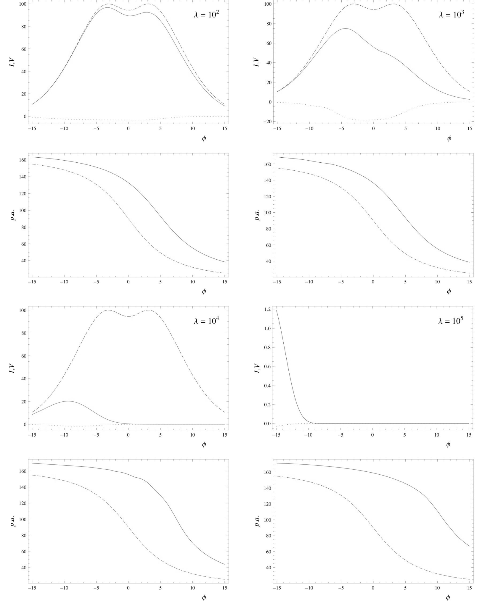
On Fig. 12 we show the p.a. swing (lower panels), the intensity (solid lines on the top panels), and the Stokes parameter (dotted lines) as a function of the pulsar phase for extraordinary wave for magnetic field model C and for various multiplicity parameter . It is obvious that the absorption increases with increasing . In most cases, the trailing part of the mean profile is absorbed (see Dyks et al. 2010 as well).
Besides, as one can see, the p.a. curves differ significantly from the RVM one (dashed lines) as growing. This property can be easily understood as well. Indeed, as the escape radius (7) increases as , for large enough the polarization properties of the outgoing waves are to be formed in the vicinity of the light cylinder, i.e., in the region with quasi-homogeneous magnetic field (see Fig. 5).
Further, as was already mentioned, the drift effect causes the p.a. curve to be shifted to the trailing part of the mean profile. It is necessary to stress that the opposite shift is to take place if we neglect the drift effect on the dielectric tensor (Andrianov & Beskin 2010; Wang et al. 2010). One can note that for high values of multiplicity parameter (i.e., for full absorption of the trailing part of the mean pulse) the observer will detect approximately constant p.a. Finally, as one can see from Eqn. (76), the maximum of circular polarization is also shifted to the trailing side, as larger deviations from the -shape produce larger circular polarization. It is not visible on this picture because the trailing side of the beam is absorbed. Thus, one can conclude that the self-consistent quantitative analysis of observational data is to include these effects into consideration.
Another point should be mentioned. It is known that correct accounting of the inverse Compton scattering of the surface X-rays can reduce the pair multiplicity significantly (see, e.g., Hibschman & Arons 2001). In this case plasmas effects on emission polarization can be negligible.
On Fig. 13 we show the same dependences for various Lorentz-factors of outgoing plasma , , and . As the escape radius (7) decreases as , the largest shift of the curve takes place for small . Finally, on Fig. 14 one can see the same dependences for various wave frequencies , , and GHz. As , the largest shift of the p.a. curve takes place for small frequencies. One can note that the full investigation of frequency dependence of mean profiles of radio pulsars is more complicate and must include, e.g., the detailed analysis of frequency dependence of the emission radius (BGI). This is beyond the scope of the article.
As was demonstrated above, in general the sign of the circular polarization remains constant for a given mode. But under certain conditions the change of the sign in the same mode may occur. It can take place when we cross the directivity pattern in the very vicinity of the magnetic axis. Such an example for the X-mode is shown on Fig. 15 for P = 1s, , , , , and . Certainly, this example is illustrative only. To explain the change of the sign of the circular polarization in the centre of the mean profile the separate consideration is necessary.

Finally, in Table 3 we present the values of maximum derivative , that is commonly used for determination of the inclination angle (see, e.g., Kuzmin & Dagkesamanskaya 1983; Malov 1990; Everett & Weisberg 2001). As we see, these values significantly depend on the plasma parameters (and can differ drastically from the RVM value). Hence, more precise specifying of magnetospheric and plasma model is necessary for quantitative analysis of the pulsar characteristics.
In our opinion, this technique can be applied in future for radio pulsars for which the whole -swing is detected. Otherwise, the situation like in Fig. 12 for may occur, when one can detect only constant part of the swing. At any way, one can conclude that if one try to fit the whole p.a. curve by the RVM function (1), then for low enough number density () and high enough particle energy () the angles and obtained will satisfy the reality. But in other cases unexpected result may occur. As shown on Fig. 16, left panel (see Table 2 as well), the simulated curve could be nicely fitted by the RVM model with non-zero shift value (1), but with the angles and that drastically differ from real ones and . On the other hand, the precision in determination of the angles and may be not so high (see Fig. 16, right panel).
| (GHz) | |||||
|---|---|---|---|---|---|
| 50 | 1 | 4.7 | |||
| 50 | 1 | 7.4 | |||
| 50 | 1 | 10.5 | |||
| 10 | 1 | 11.5 | |||
| 50 | 1 | 4.3 | |||
| 100 | 1 | 4.7 | |||
| 300 | 1 | 4.0 | |||
| 50 | 0.03 | 8.4 | |||
| 50 | 0.5 | 3.8 | |||
| 50 | 0.2 | 5.5 |
5.2 Two modes profiles

On Fig. 17 an examples of the mean profiles including two orthogonal modes are presented. The ratio of the intensities in the radiation domain was assumed to be . The jumps in the p.a. curves were done at the phase where . As we see, this jump can differ from . This results from the different trajectories of two orthogonal modes. It is necessary to stress that in our consideration the ratio is free, and its precise determination is a question for the radio emission generation theory.
We see that for radio pulsars for which two modes can be observed the mean profiles are indeed to have the triple form, which, in general, are not to be symmetric. As the O-mode deviates from magnetic axis, we have to see the O-mode in the leading part, the X-mode in the centre, and again the O-mode in the trailing part of the mean profile. The detailed comparison with observational data will be prepared in the separate paper.
5.3 Millisecond pulsars
As the last example, on Fig. 18 we show the mean profiles obtained for millisecond pulsar (the parameters are given in Table 4). One important feature appearing here is that the leading, not trailing part of the mean profile can be absorbed. It is caused by the bending of the open field lines tube near the light cylinder due to non-dipolar magnetic field. As a result, the cyclotron resonance takes place in the region of rarefired plasma for the trailing part of the pulse. Also, stronger deviations from the -shape of p.a. swing are found as compared to the case of ordinary pulsar, because the polarization forms closer to the light cylinder.

| ms | G | 0.04 | 50 |
6 Discussion and conclusions
In this paper we study the influence of the propagation effects on the mean profiles of radio pulsars. The Kravtsov-Orlov approach allows us firstly to include into consideration the transition from geometrical optics to vacuum propagation, the cyclotron absorption, and the wave refraction simultaneously. Arbitrary non-dipole magnetic field configuration, drift motion of plasma particles, and their realistic energy distribution were taken into account. Using numerical integration, we found how the propagation effects can correct the main characteristics of the hollow cone model.

To summarize, one can formulate the following results:
- •
We confirm the one-to-one correlation between the signs of circular polarization and the position angle derivative () along the profile for both ordinary and extraordinary waves. For the X-mode the signs should be the SAME, and OPPOSITE for the O-mode.
- •
The standard -shape form of the swing (1) can be realized for small enough multiplicity and large enough bulk Lorentz-factor only. In other cases the significant differences can take place. The location of the maximum derivative is shifted to the trailing side of the pulse.
- •
The value of maximum derivative , that is often used for determination the angle between magnetic dipole and rotation axis, depends on the plasma parameters [and differs from rotation vector model (RVM) value] and, hence, cannot be used without more precise specifying of magnetospheric plasma model.
- •
In general, the trailing side of the emission beam is absorbed.
In our opinion, even the preliminary consideration demonstrates that these conclusions are not in contradiction with observational data. The first statement is in good agreement with observations (Han et al. 1998; Andrianov & Beskin 2010). In some cases, the sign reversal in the core can occur (see Fig. 15 and Wang et al. 2010), that is detected for several pulsars (see also Radhakrishnan & Rankin 1990). The second point is in agreement with empirical model of Blaskiewicz et al. (1991). On the other hand, as the shift value depends on plasma parameters (assuming fixed geometry), the solution of the inverse problem (i.e., the fitting of the real pulsar profiles) can in principle provide us a chance of correct enough estimating of plasma parameters. Finally, the last point is in agreement with observations as well (see, e.g., Backus et el., 2010). In more detail, it takes place for large enough multiplicity parameter . But in some cases the leading part can be absorbed as well. It happens when the polarization forms close to the light cylinder.
Finally, Fig. 19 demonstrates our understanding of the X- and O-modes propagation in the pulsar magnetosphere. Here the dot-dash lines going to the panels with pulsar profiles show different intersections of directivity pattern, that form the observable profiles. Resulting from the different propagation, the O- and X-modes produce two concentric cones, the inner (core) part corresponding to the X-mode and the outer (conal) one to the O-mode. Remember that the analysis of the relative intensity in O- and X-modes is a question for generation theory. In the context of the present propagation theory this parameter should be considered as a free one.
Another source of uncertainty which can affect the formation of the mean profile (and, in particular, results in the formation of its more complicated shape) is the possible ”spotty” of the directivity pattern, i.e., the presence of the separate radiative domains within the diagram (Rankin 1993). As is well-known, such separate domains are observed as a subpulse drift (Ruderman & Sutherland 1975, Deshpande & Rankin 2001).
In addition, the full analysis is to include the possible linear depolarization. E.g., depolarization at the edges of the profile can be easily interpreted as a mixing of X and O-modes (Rankin & Ramachandran 2003). But the total degree of linear polarization (e.g., if we clearly see only one mode) is a question to propagation in the generation region. If this region is rather thick then one can expect the possible depolarization. For this reason we do not treat here the total degree of linear polarization at all.
As we see, in general if only one mode dominates in pulsar profile, then we expect statistically (double) mean profile for the O-mode and (single) one for the X-mode. Of course, we suppose here that there is nonzero natural width of the radiative domains that efficiently smooths the hollow cone corresponding to the narrow X-mode. Nevertheless, as is shown on Fig. 19, the X-mode can in principal produce profile and O-mode can produce ones. The and profiles can be obtained when only X-mode is produced in the formation region. On the other hand, if there are two modes with the similar intensity, the triple (T) and multiple (M) profiles can be obtained as well. So, this picture is in agreement with Rankin’s morphological classification (Rankin 1983). Our investigation provides an additional information to morphological structure, i.e., the information of the type of the mode that forms mainly the mean profile. As was demonstrated, only the correlation between derivative and signs provides us this chance.
Finally, the determination of the angular dimension of the core and conal beams depends greatly on the emission radius (i.e., again, on the generation mechanism). So the detailed analysis is also beyond the scope of current investigation (one can find empirical results on this in, e.g., Maciesiak & Gil 2011).
Thus, the approach developed in this paper allows the predictions of the theory of radio emission to be quantitatively compared with the observational data. Moreover, based on the observational data, one can reject a number of models in which the shapes of the profiles of the position angle and the degree of circular polarization never realized in practice are obtained. Thus, it becomes possible to solve the inverse problem, i.e., to determine the parameters of the outflowing plasma and the magnetic field structure.
We will be glad to any collaboration with observers for investigating the observational features of the mean profiles on the base of our theory. The source code of our calculations (in Mathematica 7 or C) is available under request.
7 Acknowledgments
We thank Prof. A.V. Gurevich and Ya.N. Istomin for his interest and support, and J. Dyks, A. Jessner, P. Jaroenjittichai, M. Kramer, V.V. Kocharovsky, D. Mitra, M.V. Popov, R. Shcherbakov, B. Rudak, and H.-G. Wang for useful discussions. We also thank A. Spitkovsky for valuable opportunity and assistance in dealing with his numerical solution and for outstanding discussions. This work was partially supported by Russian Foundation for Basic Research (Grant no. 11-02-01021).
Appendix A Refraction

In this work we consider the simple model of the refraction obtained under the assumption that the plasma number density is constant within the polar cap, i.e., . To include refraction into consideration we introduce the ”imaginary source” of radiation giving the same trajectory at large distances whence emitted parallel to the magnetic field line (see Fig. 20). As the ”tearing off” level locates deeply in the magnetosphere, i.e., , one can use the analytical expression (21) for the angle (BGI 1993). It gives for the polar angle of the emission point
| (78) |
(for dipole magnetic field it does not depend on the radial distance). As a result, we obtain for the polar angle of imaginary source
| (79) |
After some algebraic calculations, one can find the trajectory
Here
| (80) |
is the radius of imaginary source, and
| (81) |
where
| (82) |
Finally, is a unit vector perpendicular to lying for every pulsar phase in the plane containing the magnetic and the wave vectors.
Appendix B Derivation of dielectric tensor
Since all the quantities in equation (27) are proportional to , its solution can be easily obtained:
| (83) | |||||
| (84) | |||||
| (85) |
where
| (86) | |||||
| (87) |
From (30) one can find the number density pertubation
| (88) |
After making substitution to (31) we obtain for dielectric tensor components:
| (89) | |||||
| (90) | |||||
| (91) | |||||
| (92) | |||||
| (93) | |||||
| (94) | |||||
| (95) |
Here the quantity . Other components of the permittivity tensor are defined by its hermiticity. Therefore, in the expression for gyrofrequency
we should take into the account the sign of the charge . One can check that moving to the appropriate reference frame this dielectric tesor reduces to the well-known one (Godfray et al. 1975; Suvorov & Chugunov 1975; Hardee & Rose 1975) obtained for the case . Finally, as we see, the cyclotron resonance corresponds to the condition .
| (96) | |||||
| (97) | |||||
| (98) | |||||
| (99) | |||||
| (100) | |||||
| (101) |
Appendix C Rotation of coordinate systems
The equations of the transition of the dielectric tensor from the coordinate system formulated in Sect. 3 to that used in Sect. 4 are the following
Here is the angle between the ray propagation and local magnetic field directions. Other components of the tensor can be defined by its hermiticity.
Appendix D Natural modes
For obtaining naturals modes of tensor it is convenient to rotate the coordinate frame in xy-plane to make the condition to be valid. One can find that it can be done by rotation defined by the following matrix:
where
| (102) |
In this frame the corresponding expressions for tensor components (defining as ) are:
The naturals modes for this tensor (with pure imaginary x’y’ component) are well-known (Andrianov & Beskin 2010; Wang et al. 2010):
| (103) | |||||
| (104) |
where by the definition
| (105) |
It can be easily shown that in our case
| (106) |
Hence, Eqns. (72)-(73) really define the natural modes in the laboratory frame. The simple expression, which corresponds to a zero plasma temperature for is the following (cf. Melrose & Luo 2004 for zero drift):
| (107) |
References
- Andrianov & Beskin (2010) Andrianov A.S., Beskin V.S., 2010, Astron. Lett., 36, 248
- Arons & Scharlemann (1979) Arons J., Scharlemann E.T., 1979, Astrophys. J., 231, 854
- Asseo (1995) Asseo E., 1995, MNRAS, 276, 74
- Asseo (1980) Asseo E., Pellat R., Rosado M., 1980, Astrophys. J., 239, 661
- Bacus, Mitra & Rankin (2010) Backus I., Mitra D., Rankin J., 2010, MNRAS, 404, 30
- Barnard (1986) Barnard J.J., 1986, Astrophys. J., 303, 280
- Barnard & Arons (1986) Barnard J.J., Arons J., 1986, Astrophys. J., 302, 138
- Beskin (1999) Beskin V.S., 1999, Physics-Uspekhi, 169, 1169
- Beskin (2009) Beskin V.S., 2009, MHD Flows in Compact Astrophysical Objects, Springer, Berlin
- Beskin (2010) Beskin V.S., 2010, Physics-Uspekhi, 180, 1241
- Beskin, Gurevich & Istomin (1988) Beskin V.S., Gurevich A.V., Istomin Y.N., 1988, Astrophys. and Space Sci., 146, 205
- Beskin & Gurevich & Istomin (1993) Beskin V.S., Gurevich A.V., Istomin Y.N., 1993, Physics of the Pulsar Magnetosphere, Cambridge University Press, Cambridge (BGI)
- Blandford (1975) Blandford R.D., 1975, MNRAS, 170, 551
- Blaskiewicz, Cordes & Wasserman (1991) Blaskiewicz M., Cordes J.M., & Wasserman I, 1991, Astrophys. J., 370, 643
- Bogovalov (1999) Bogovalov S.V., 1999, Astron. Astrophys., 349, 1017
- Broderick & Blandford (2010) Broderick A.E., Blandford R.D., 2010, ApJ, 718, 1085
- Budden (1972) Budden K.G., 1972, J. Atm. Terr. Phys., 34, 1909
- Cheng & Ruderman (1979) Cheng A.F., Ruderman M.A., 1979, Astrophys. J., 229, 348
- Contopoulos, Kazanas & Fendt (1999) Contopoulos I., Kazanas D., Fendt Ch., 1999, Astrophys. J., 511, 35
- Kravtsov (2007) Czyz Z.H., Bieg B., Kravtsov Yu.A., 2007, Phys. Lett. A, 368, 101
- Daugherty & Harding (1982) Daugherty J.K., Harding A.K., 1982, Astrophys. J, 252, 337
- Dishpande & Rankin (2001) Deshpande A.A., Rankin J., 2001, MNRAS, 322, 438
- Dyks (2010) Dyks J., Wright G.A.E., Demorest P.B., 2010, MNRAS, 405, 509
- Everett & Weisberg (2001) Everett J.E., Weisberg J.M., 2001, ApJ, 553, 341
- Fussel, Luo & Melrose (1999) Fussel D., Luo Q., Melrose D.B., 2003, MNRAS, 343, 1248
- Ginzburg (1961) Ginzburg V.L., 1961, Propagation of Electromagnetic Waves in Plasma, Gordon & Breach Science Publishers, New York
- Godfray, Shanahan & Thode (1975) Godfray B.B., Shanahan W.R., Thode L.E., 1975, Phys. Fluids, 18, 346
- Goldreich (1971) Goldreich P., Keeley D.A., 1971, Astrophys. J., 170, 463
- Gruzinov (2006) Gruzinov A., 2006, ApJ, 647, 119
- Gurevich & Istomin (1985) Gurevich A.V., Istomin Y.N., 1985, Sov. Phys. JETP, 62, 1
- Hankins & Rankin (2010) Hankins T.H., Rankin J.M., 2010, AJ, 139, 168
- Han (1998) Han J., Manchester R., Xu R., Qiao G., 1998, MNRAS, 352, 915
- Hardee & Rose (1975) Hardee Ph.D., Rose W.K., 1975, Astrophys. J., 210, 533
- Hibsch (2001) Hibschman J.A., Arons J., 2001, Astrophys. J., 546, 382
- Istomin (1988) Istomin Y.N., 1988, Sov. Phys. JETP, 67, 1380
- IstoSo (2009) Istomin Y.N., Sobyanin D.N., 2009, Phys. JETP, 109, 393
- Kazbegi (1991) Kazbegi A.Z., Machabeli G.Z., Melikidze, G. I., 1991, MNRAS, 253, 377
- Keith et al. (2010) Keith M. J., Johnston S., Weltevrede P., Kramer M., 2010, MNRAS, 402, 745
- KrB (2008) Kravtsov Yu.A., Bieg B., 2008, Cent. Eur. J. Phys., 6, 563
- Kravtsov & Orlov (1990) Kravtsov Yu.A., Orlov Yu.I., 1990, Geometrical Optics of Inhomogeneous Media, Springer, Berlin
- Kuzmin & Dagkesamanskaya (1983) Kuzmin A. D., Dagkesamanskaya I. M., 1983, Sov. Astron.Lett., 9, 80
- Landau & Lifshits (1975) Landau L.D., Lifshits E.M., 1975, The Classical Theory of Fields, Pergamon Press, Oxford
- Luo, Melrose & Machabeli (1994) Luo Q., Melrose D.B., Machabeli G. Z., 1994, MNRAS, 268, 159
- Lyubarskii (1996) Lyubarskii Yu.E., 1996, Astron. Astrophys., 308, 809
- Lyubarskii (2008) Lyubarskii Yu.E., 2008, AIP Conference Proceedings, 983, 29-37
- Lyne & Graham-Smith (1998) Lyne A.G., Graham-Smith F., 1998, Pulsar Astronomy, Cambridge University Press
- MGil (2011) Maciesiak K., Gil J., 2011, MNRAS, 417, 1444
- Malov (1990) Malov I.F., 1990, Sov. Astron., 34, 189
- Manchester & Taylor (1977) Manchester R., Taylor J., 1977, Pulsars, Freeman, San Francisco
- Medin & Lai (2010) Medin Z., Lai D., 2010, MNRAS, 406, 1379
- MelroseL (2004) Melrose D.B., Luo Q., 2004, MNRAS, 352, 915
- Michel (1973) Michel F.C., 1973, Astrophys. J., 180, L133
- Mikhailovsky et al. (1982) Mikhailovsky A.B., Onishchenko O.G., Suramlioshvili G.I., Sharapov S.E., 1982, Sov. Astron. Lett., 8, 685
- Mitra &Melikidze (2009) Mitra D., Gil J., Melikidze G., 2009, Astrophys. J., 696, 2
- Mitra &Rankin (2011) Mitra D., Rankin J., 2011, Astrophys. J., 727, 92
- Petrova (2001) Petrova S.A., 2001, Astron. Astrophys. 378, 883
- Petrova (2001) Petrova S.A., 2003, Astron. Astrophys. 408, 1057
- Petrova (2006) Petrova S.A., 2006, MNRAS 368, 1764
- Petrova & Lyubarskii (1998) Petrova S.A., Lyubarskii Yu.E., 1998, Astron. Astrophys., 333, 181
- Petrova & Lyubarskii (2000) Petrova S.A., Lyubarskii Yu.E., 2000, Astron. Astrophys., 355, 1168
- RadCo (1969) Radhakrishnan V., Cocke D.J., 1969, Astrophys. Lett., 3, 225
- RankinR (1990) Radhakrishnan V., Rankin J., 1990, Astrophys. J., 352, 258
- Rankin (1983) Rankin J., 1983, Astrophys. J., 274, 333
- Rankin (1990) Rankin J., 1990, Astrophys. J., 352, 247
- Rankin (2003) Rankin J., Ramachandran R., 2003, Astrophys. J., 590, 411
- Ruderman & Sutherlend (1975) Ruderman M.A., Sutherlend P.G., 1975, Astrophys. J., 196, 51
- Sazonov (1969) Sazonov V.N., 1969, Sov. Phys. JETP, 29, 578
- Shcherbakov (2011) Shcherbakov R.V., Huang L., 2011, MNRAS, 410, 1052
- Spitkovsky (2006) Spitkovsky A., 2006, Astrophys. J., 648, L51
- Sturrock (1971) Sturrock P.A., 1971, Astrophys. J., 164, 529
- Suvorov & Chugunov (1975) Suvorov E.V., Chugunov Yu.M., 1975, Astrophysics, 11, 203
- Taylor & Stinebring (1986) Taylor J.H., Stinebring D.R., 1986, Ann. Rev. Astron. Astrophys., 24, 285
- Timokhin (2006) Timokhin A.N., 2006, MNRAS, 368, 1055
- Usov (2006) Usov V.V., 2006, Proceedings of the 26th meeting of the IAU, Prague, Czech Republic
- Wang & Lai &Han (2010) Wang Z., Lai D., Han J., 2010, MNRAS, 403, 2
- Wang & Lai &Han (2010) Wang Z., Lai D., Han J., 2011, MNRAS, 417, 1183
- Weltevrede & Johnston (2008) Weltevrede P., Johnston S., 2008, MNRAS, 391, 1210
- Yan et al. (2011) Yan W. M., Manchester R.N., van Straten W. et al. 2011, MNRAS, 414, 2087
- Zheleznyakov (1964) Zheleznyakov V.V., 1970, Radio Emission of the Sun and Planets, Pergamon, Oxford
- Zheleznyakov (1977) Zheleznyakov V.V., 1996, Radiation in Astrophysical Plasmas, Springer, Berlin
- Zheleznyakov, Kocharovsky & Kocharovsky (1983) Zheleznyakov V.V., Kocharovsky V.V., Kocharovsky Vl.V., 1983, Sov. Phys. Uspekhi, 141, 257