Two-loop renormalization of three-quark operators in QCD

The studies of hard exclusive processes including baryons will constitute a significant part of the experimental program at the planned new facilities at JLAB (Newport News) and FAIR (Darmstadt). QCD description of such reactions and also heavy hadron weak decays with light baryons in the final state (LHCB, CERN) involves baryon wave functions at small transverse separations, the so-called distribution amplitudes (DA). The nucleon DAs already have received considerable attention in the literature, see e.g. Refs. [1, 2, 3, 4]. In particular lattice calculations can provide one with reliable estimates of the lowest moments of baryon DAs which are defined by matrix elements of local three-quark operators [5, 6].

As usually, the QCD matrix elements depend on the scale and on the renormalization scheme. The renormalization of baryon operators in dimensional regularization beyond the leading logarithms involves some subtleties that, to our knowledge, have not been treated in the literature in a systematic way and the purpose of our letter is to fill this gap. Our study was fuelled in particular by the need to calculate the NLO $\overline{\text{MS}}/\text{MOM}$ scheme conversion factors in lattice studies (cf. [7, 8]) and the NLO extensions of light-cone sum rule calculations of baryon form factors [9] which have already started [10].

It is well known that for a generic operator the widely used $\overline{\text{MS}}$ prescription does not fix a renormalization scheme completely. Indeed, for a noninteger dimension $d$ the Lorentz group $SO(1,d-1)$ becomes infinite dimensional. As a consequence the tensor content of the $d-$dimensional theory is richer than that of a strictly four dimensional one. In particular, it means that there exist operators in $d-$dimensions which have no counterparts in four dimensions, e.g. totally antisymmetric tensors of rank $n>4$. Such operators vanish in $d=4$ and are conventionally referred to as evanescent operators. However, one cannot simply exclude evanescent operators from consideration since under renormalization they mix with the physical operators. The situation was thoroughly analyzed by Dugan and Grinstein [11]. They have shown that one can always get rid of the mixing by a suitable finite renormalization. A more detailed discussion in [12] shows that such finite renormalization is not unique.

We are interested in the renormalization of the local three-quark operator

$\displaystyle\mathcal{Q}^{abc}_{\alpha\beta\gamma}=\epsilon^{ijk}q^{ia}_{\alpha}\,q^{jb}_{\beta}\,q^{kc}_{\gamma}\,.$

(1)

Here $\alpha,\beta,\gamma$ are the spinor indices, while $ijk$ and $abc$ are the color and flavor indices of the quark fields, respectively. The flavor structure of the operator will be irrelevant for the further discussion, so that from now on we will suppress the flavor indices. In typical applications one usually tries to get rid of multiple spinor indices by contracting (1) with suitable $\gamma-$matrices. An example is provided by the so – called Ioffe current [13]

$$\eta_{I}(x)=\epsilon^{ijk}\left[u^{i}(x)C\gamma_{\mu}u^{j}(x)\right]\gamma_{5}\gamma^{\mu}d^{k}(x)\,,$$

(2)

or the leading twist nucleon operator

$\displaystyle\eta_{N}(x)=\epsilon^{ijk}\left[u^{i}(x)C\not{z}u^{j}(x)\right]\not{z}d^{k}(x)\,.$

(3)

Here $z$ is a light-like auxiliary vector and $C$ is the charge conjugation matrix. The two-loop anomalous dimension of the Ioffe current was calculated in [14]. Evanescent operators do not contribute at this order to the current (2) due to special cancelations however they should be taken into account for the current (3).

The renormalization of the currents (2), (3) is not of academic interest only ¹¹ 1 The maximal helicity three-quark operators in the $\mathcal{N}=4$ SUSY were studied in Refs. [15, 16] in AdS/CFT context.. The sum rules involving these currents provide an important tool for quantitative study of hadronic properties, see e.g. Refs. [2, 9, 13, 17]. The matrix elements of the operator (1) and the corresponding interpolating currents satisfy at tree level certain symmetry relations which are derived with help of Fierz transformations [3]. Therefore it is preferable to use a renormalization scheme which respects these relations.

In our opinion the scheme developed in  [11, 12, 14] is not best suited for renormalization of the three-quark operators. We will suggest a different scheme and calculate the two-loop anomalous dimensions of the operator (1) in this scheme.

The paper is organized as follows: In Sect. 2 we briefly review the renormalization approach taken by Dugan and Grinstein [11]. Then we propose a new renormalization scheme and discuss its properties. In Sect. 3 we present the results of the calculation of anomalous dimensions of the operator (1) in two loops. Conclusions are presented in Sect. 4.

Let us at first discuss the renormalization of the Ioffe current in the scheme [11]. It will be more convenient to work with the current $\bar{\eta}_{1}(x)=\gamma_{5}\eta_{I}(x)$ which definition does not involve the matrix $\gamma_{5}$. Next, we will assume that the $d-$dimensional charge conjugation matrix $C$ satisfies the defining relation $C\gamma_{\mu}C^{-1}=-\gamma^{T}_{\mu}$. Then one can easily verify that the operator $\bar{\eta}_{1}$ mixes under renormalization with the operators

$\displaystyle\bar{\eta}_{n}=\epsilon^{ijk}\left[u^{i}C\gamma^{(n)}u^{j}\right]\gamma^{(n)}d^{k}\,,$

(4)

$n$ odd. Here $\gamma^{(n)}\otimes\gamma^{(n)}\equiv\gamma^{(n)}_{\mu_{1}\ldots\mu_{n}}\otimes\gamma^{(n)}_{\mu_{1}\ldots\mu_{n}}$ and $\gamma^{(n)}_{\mu_{1}\ldots\mu_{n}}$ is the antisymmetrized product of $n$ gamma matrices, $\gamma^{(n)}_{\mu_{1}\ldots\mu_{n}}=\gamma_{[\mu_{1}}\ldots\gamma_{\mu_{n}]}\,.$

The renormalized operators $\bar{\eta}_{n}$ take the form ²² 2 In the $\overline{\text{MS}}$ scheme the renormalization matrix $Z$ is a series in $1/\epsilon$.

$\displaystyle[\bar{\eta}_{n}]=\sum_{k=1,3\ldots}Z_{nk}\bar{\eta}_{k}\,.$

(5)

Here and below the square brackets will denote a renormalized operator.

In $d-$dimensions all operators (4) are independent and satisfy the standard RG equation

$\displaystyle\Big([M\partial_{M}+\beta(\alpha_{s})\partial_{\alpha_{s}}]\delta_{nk}+\gamma_{nk}\Big)[\bar{\eta}_{k}]=0\,.$

(6)

Here $M$ is the renormalization scale, $\beta(\alpha_{s})$ is the beta function and $\gamma_{nk}$ is the anomalous dimension matrix

$\displaystyle\gamma=-M\left(\frac{d}{dM}\mathbb{Z}\right)\,\mathbb{Z}^{-1}\,,$

$\displaystyle\mathbb{Z}=ZZ_{q}^{-3}\,$

(7)

with $Z_{q}$ being the quark field renormalization constant, $q_{0}=Z_{q}q$.

Generic correlation functions with insertion of the operator $\bar{\eta}_{n}$, $n>3$, vanish at tree level in $d=4$, thus these operators are evanescent ones. However, it does not hold anymore beyond the tree level approximation. Moreover, even if the evanescent operators were zero at one scale they would reappear at another scale due to mixing with physical operators.

It was shown in [11] that making a finite renormalization one can ensure vanishing of evanescent operators beyond tree level at any scale. In other words this means that in an arbitrary scheme the evanescent operators $\bar{\eta}_{n}$, $n>3$ can be expressed in $d=4$ in terms of the first two, "physical", operators $\bar{\eta}_{1}$ and $\bar{\eta}_{3}$ ³³ 3 Strictly speaking one can choose any other two operators as the basic (physical) ones, however in this case the expansion coefficients $a_{nk}$ will be singular in $\alpha_{s}$.

$\displaystyle[\bar{\eta}_{n}]=a_{n1}(\alpha_{s})[\bar{\eta}_{1}]+a_{n3}(\alpha_{s})[\bar{\eta}_{3}],$

$\displaystyle n>3\,.$

(8)

The above identity should be understood as an equality between arbitrary correlation functions of the operators on the l.h.s and on the r.h.s of this equation. (To avoid misunderstanding we remind that taking the limit $d\to 4$ one puts $\gamma^{(n)}=0$ for $n>4$ in the renormalized correlation functions.)

The proof of Eq. (8) given in Ref. [11] employs combinatorics of the $R-$operation. It was done on the example of the four-fermion operators but the argumentation is quite general. Another way to verify Eq. (8) is to note that in some nonminimal schemes, e.g. the MOM$-$scheme, the condition $[\bar{\eta}_{n}]=0$ for $n>3$ holds automatically. Operators in any two scheme are related by a finite renormalization that implies Eq. (8).

Inserting (8) into (6) one derives the RG equation involving the physical operators $\bar{\eta}_{1,3}$ only

$\displaystyle\Big([M\partial_{M}+\beta(\alpha_{s})\partial_{\alpha_{s}}]\delta_{nk}+\tilde{\gamma}_{nk}\Big)[\bar{\eta}_{k}]=0\,,$

(9)

where the indices $n,k$ take the values $1,3$ and

$\displaystyle\tilde{\gamma}_{nk}=\gamma_{nk}+\sum_{p=5,7\ldots}\gamma_{np}a_{pk}\,.$

(10)

Evidently one has to consider the evanescent operators in order to obtain the correct result for the anomalous dimension matrix.

It is also clear that if the operators $\bar{\eta}_{n}$ enter the OPE of certain currents in $d-$dimensions, the four dimensional OPE can be written in terms of the physical operators only with the coefficient functions being appropriately modified.

In this work we propose a different $\overline{\text{MS}}$ scheme for the renormalization of the three-quark operator (1) (see also the recent paper [18]). Our analysis follows closely the approach taken in [19]. Instead of contracting the operator (1) with different $\gamma-$matrices we will consider the operator with open spinor indices. The divergent part of any diagram contributing to the correlator

$\displaystyle\langle{Q_{\alpha\beta\gamma}(0)\bar{q}_{\alpha^{\prime}}(k)\bar{q}_{\beta^{\prime}}(p)\bar{q}_{\gamma^{\prime}}(q)}\rangle$

(11)

after subtracting the sub-divergences can be cast into the form

$\displaystyle\sum_{nmk}f_{nmk}(\epsilon)\,(\Gamma_{nmk})^{\alpha^{\prime}\beta^{\prime}\gamma^{\prime}}_{\alpha\beta\gamma}\,,$

(12)

where the functions $f_{nmk}(\epsilon)$ are series in $1/\epsilon$. The gamma matrix structures $\Gamma_{nmk}$ are defined by

$\displaystyle(\Gamma_{nmk})^{\alpha^{\prime}\beta^{\prime}\gamma^{\prime}}_{\alpha\beta\gamma}=\gamma^{(n)}_{\alpha\alpha^{\prime}}\otimes\gamma^{(m)}_{\beta\beta^{\prime}}\otimes\gamma^{(k)}_{\gamma\gamma^{\prime}}\,,$

(13)

where it is assumed that all Lorentz indices of gamma matrices ($\gamma^{(n)}_{\mu_{1}\ldots\mu_{n}}$) are contracted between themselves ⁴⁴ 4 There is only one nontrivial way to contract all indices.. We define the subtraction scheme by removing all singular terms (12) from the correlator (11). Thus the renormalized operator $\mathcal{O}_{\alpha\beta\gamma}$ takes the form

$\displaystyle[\mathcal{O}_{\alpha\beta\gamma}]=Z_{\alpha\beta\gamma}^{\alpha^{\prime}\beta^{\prime}\gamma^{\prime}}\mathcal{O}_{\alpha^{\prime}\beta^{\prime}\gamma^{\prime}},$

(14)

where

$\displaystyle Z_{\alpha\beta\gamma}^{\alpha^{\prime}\beta^{\prime}\gamma^{\prime}}=1+\sum_{nmk}a_{nmk}(\epsilon)\,(\Gamma_{nmk})^{\alpha^{\prime}\beta^{\prime}\gamma^{\prime}}_{\alpha\beta\gamma}$

(15)

and

$\displaystyle a_{nmk}(\epsilon)=\sum_{p=1}^{\infty}{\epsilon^{-p}}\,a_{nmk}^{(p)}(\alpha_{s})\,.$

(16)

The RG equation for the operator $[\mathcal{O}_{\alpha\beta\gamma}]$ reads

$\displaystyle\Big(M\partial_{M}+\beta(\alpha_{s})\partial_{\alpha_{s}}\Big)[\mathcal{O}_{\alpha\beta\gamma}]=-\gamma^{\alpha^{\prime}\beta^{\prime}\gamma^{\prime}}_{\alpha\beta\gamma}[\mathcal{O}_{\alpha^{\prime}\beta^{\prime}\gamma^{\prime}}]\,,$

(17)

where the anomalous dimension matrix $\gamma$ is given by Eq. (7). Calculating the inverse matrix $Z^{-1}$ one has to carry out all gamma matrix algebra in $d-$dimensions and this results in emergence of $\epsilon-$regular contributions in $Z^{-1}$. Thus the matrix $Z^{-1}$ contains both singular and regular terms in $\epsilon$

$\displaystyle(Z^{-1})_{\alpha\beta\gamma}^{\alpha^{\prime}\beta^{\prime}\gamma^{\prime}}=1+\sum_{nmk}\tilde{a}_{nmk}(\epsilon)\,(\Gamma_{nmk})^{\alpha^{\prime}\beta^{\prime}\gamma^{\prime}}_{\alpha\beta\gamma}\,,$

(18)

with $\tilde{a}_{nmk}(\epsilon)=\sum_{p=-\infty}^{\infty}{\epsilon^{-p}}\,\tilde{a}_{nmk}^{(p)}(\alpha_{s})\,.$ This is different from the standard situation where $Z^{-1}$ is a series in $1/\epsilon$, $Z^{-1}=\sum_{k}\tilde{a}_{k}(1/{\epsilon}^{k})$ and there are no finite in $\epsilon$ terms.

The anomalous dimension matrix $\gamma$ in $d-$dimensions takes the form similar to (15)

$\displaystyle\gamma=\sum_{nmk}\gamma_{nmk}(\alpha_{s},\epsilon)\,\Gamma_{nmk}\,,$

(19)

(we omitted the spinor indices for brevity). The coefficients $\gamma_{nmk}(\alpha_{s},\epsilon)$ are regular functions of $\alpha_{s}$ and $\epsilon$. In $d=4$ one can drop all $\Gamma-$matrices which vanish in four dimensions from the sum (19), i.e. $n,m,k\leq 4$.

Let us see what happens with evanescent operators in this scheme. We define the renormalized current $[\bar{\eta}_{n}]$ as follows

$\displaystyle[\bar{\eta}_{n}]=(C\gamma^{(n)})_{\alpha\beta}\otimes\gamma^{(n)}_{\gamma^{\prime}\gamma}\,[\epsilon^{ijk}u^{i}_{\alpha}u^{j}_{\beta}d^{k}_{\gamma}]\,.$

(20)

Since the $\gamma-$matrix structure is convoluted with the renormalized (finite) operator, one can safely put $\gamma^{(n)}=0$ for $n\geq 5$ in $d=4$. Thus, the evanescent operators automatically vanish in $d=4$ in this scheme and we can treat the renormalized operator $[\mathcal{O}_{\alpha\beta\gamma}]$ as a pure four dimensional object. Since the $\gamma-$matrices in Eq. (20) are already four dimensional one avoids the problem of defining the matrix $\gamma_{5}$ in $d-$dimensions. Moreover, this scheme is obviously consistent with the Fierz identities, as all contractions of the renormalized operator with $\gamma-$matrices are done in four dimensions.

In this section we present results of the two-loop calculation of the anomalous dimension matrix for the three-quark operator (1). All calculations were done in Feynman gauge. The quark field renormalization constant $Z_{q}$ in this gauge reads [20]

	$\displaystyle Z_{q}=$	$\displaystyle 1-\frac{a}{2\epsilon}C_{F}+\frac{a^{2}}{2}\biggl[\frac{1}{\epsilon^{2}}\left(\frac{1}{4}C_{F}^{2}+C_{F}C_{A}\right)$
		$\displaystyle+\frac{1}{\epsilon}C_{F}\left(-\frac{17}{4}C_{A}+\frac{3}{4}C_{F}+\frac{1}{2}N_{f}\right)\biggr]\,.$		(21)

Here $a=\alpha_{s}/(4\pi)$, $C_{F}=(N_{c}^{2}-1)/2N_{c}$, $C_{A}=N_{c}$ and $N_{f}$ is the number of flavors. The beta function for the coupling $a$ is

$\displaystyle\beta_{a}(a)=M\frac{da}{dM}=-2\epsilon a+2b_{0}a^{2}+O(a^{3})\,,$

(22)

where $b_{0}=2N_{f}/3-11/3N_{c}$.

The expression for the anomalous dimension matrix (7) takes the form

	$\displaystyle\gamma=$	$\displaystyle 2a\biggl\{\epsilon{\mathbb{Z}}^{(1)}+a\Big(\epsilon\Big[2{\mathbb{Z}}^{(2)}-{\mathbb{Z}}^{(1)}{\mathbb{Z}}^{(1)}\Big]$
		$\displaystyle\phantom{2a}-b_{0}{\mathbb{Z}}^{(1)}\Big)\biggl\}+O(a^{3})\,,$		(23)

where

$\displaystyle\mathbb{Z}=ZZ_{q}^{-3}=1+a\,\mathbb{Z}^{(1)}+a^{2}\mathbb{Z}^{(2)}+O(a^{3}).$

(24)

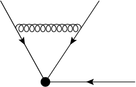
Calculating the one-loop diagram shown in Fig. 1 one gets the following expression for the renormalization matrix $Z^{(1)}$ ($Z=1+\sum a^{k}Z^{(k)}$)

$\displaystyle Z^{(1)}=-\frac{1}{6\epsilon}\Big[\Gamma_{220}+\Gamma_{202}+\Gamma_{022}+12\Big]\,,$

(25)

where

$\displaystyle\Gamma_{220}=\gamma^{(2)}_{\mu\nu}\otimes\gamma^{(2)}_{\mu\nu}\otimes I$

(26)

and similarly for the others. The one-loop anomalous dimension matrix (23) takes the form

$\displaystyle\gamma=-\frac{a}{3}\Big[\Gamma_{220}+\Gamma_{202}+\Gamma_{022}\Big]\,.$

(27)

In order to present the results of the two-loop calculations in a compact form we introduce short–hand notations for combinations of $\gamma-$matrix structures which appear in the calculations

		$\displaystyle\mathbb{C}_{2}=\,\Gamma_{220}+\Gamma_{202}+\Gamma_{022}\,,$
		$\displaystyle\mathbb{C}_{4}=\,\Gamma_{440}+\Gamma_{404}+\Gamma_{044}\,,$
		$\displaystyle\mathbb{C}_{42}=\Gamma_{422}+\Gamma_{242}+\Gamma_{224}\,,$		(28)

where

	$\displaystyle\Gamma_{440}=$	$\displaystyle\gamma^{(4)}_{\mu_{1}\mu_{2}\mu_{3}\mu_{4}}\otimes\gamma^{(4)}_{\mu_{1}\mu_{2}\mu_{3}\mu_{4}}\otimes I\,,$
	$\displaystyle\Gamma_{422}=$	$\displaystyle\gamma^{(4)}_{\mu_{1}\mu_{2}\mu_{3}\mu_{4}}\otimes\gamma^{(2)}_{\mu_{1}\mu_{2}}\otimes\gamma^{(2)}_{\mu_{3}\mu_{4}}\,.$

The contributions to the matrix $Z$ from the two-loop diagrams read

	$\displaystyle Z^{(2a)}=$	$\displaystyle-\frac{2}{9}\left\{\frac{1}{\epsilon^{2}}\Big[\mathbb{C}_{2}+12\Big]+\frac{1}{2\epsilon}\mathbb{C}_{2}\right\}\,,$
	$\displaystyle Z^{(2b)}=$	$\displaystyle\frac{1}{3}\left\{\frac{5}{4}\left(\frac{1}{\epsilon^{2}}-\frac{17}{30\epsilon}\right)-\frac{N_{f}}{6}\left(\frac{1}{\epsilon^{2}}-\frac{1}{6\epsilon}\right)\right\}\mathbb{C}_{2}\,,$
	$\displaystyle Z^{(2c)}=$	$\displaystyle-\frac{1}{36}\left\{\frac{1}{\epsilon^{2}}\Big[\mathbb{C}_{2}+12\Big]+\frac{5}{2\epsilon}\mathbb{C}_{2}\right\}\,,$
	$\displaystyle Z^{(2d)}=$	$\displaystyle\frac{3}{4}\left\{\frac{1}{\epsilon^{2}}\Big[\mathbb{C}_{2}+12\Big]+\frac{1}{\epsilon}\left(\frac{1}{6}\mathbb{C}_{2}-4\right)\right\}\,,$
	$\displaystyle Z^{(2e)}=$	$\displaystyle\frac{1}{\epsilon}\frac{5}{144}\Big\{\mathbb{C}_{4}-4\mathbb{C}_{2}-24\Big\}\,,$
	$\displaystyle Z^{(2f)}=$	$\displaystyle\frac{1}{36}\biggl\{\frac{1}{\epsilon^{2}}\left(\frac{1}{2}\mathbb{C}_{4}+8\mathbb{C}_{2}+60\right)$
		$\displaystyle\phantom{36}-\frac{1}{\epsilon}\left(\frac{1}{4}\mathbb{C}_{4}+12\mathbb{C}_{2}+120\right)\biggr\}\,,$
	$\displaystyle Z^{(2g)}=$	$\displaystyle\frac{1}{36}\biggl\{\frac{1}{\epsilon^{2}}\left(\mathbb{C}_{42}+6\mathbb{C}_{2}+48\right)$
		$\displaystyle\phantom{36}-\frac{1}{\epsilon}\left(\frac{1}{2}\mathbb{C}_{42}+\mathbb{C}_{2}\right)\biggr\}\,.$		(29)

Here the factor $Z^{(2a)}$ $(Z^{(2b)})$ comes from the quark (gluon) self-energy corrections to the one-loop diagram shown in Fig. 1. Similarly, $Z^{(2c)}$ and $Z^{(2d)}$ correspond to the QED – like and QCD – like vertex corrections, respectively. $Z^{(2e)}$ and $Z^{(2f)}$ result from to the diagrams with intersecting and non – intersecting gluon lines, respectively. Finally, $Z^{(2g)}$ takes into account contributions from the diagrams with all three quarks interacting ⁵⁵ 5 The diagram where all quark lines connected via triple gluon vertex vanishes because of the color structure..

The calculations are straightforward so we will not present them. Some useful identities for the $d$–dimensional $\gamma$–matrices can be found in Refs. [11, 21]. We also checked that our results are consistent with the two-loop calculations of Pivovarov and Surguladze [14].

Substituting (29) and (21) into (23) and taking into account the identity

$\displaystyle\mathbb{C}_{42}=\frac{1}{2}\mathbb{C}_{2}^{2}-\frac{1}{2}\mathbb{C}_{4}-2(d-3)\mathbb{C}_{2}-3d(d-1)$

one obtains for the anomalous dimension matrix in $d=4$

	$\displaystyle\gamma=$	$\displaystyle-\frac{a}{3}\mathbb{C}_{2}-\left(\frac{a}{6}\right)^{2}\biggl\{\mathbb{C}_{2}^{2}-{5}\mathbb{C}_{4}-2(b_{0}-36)\mathbb{C}_{2}\biggr\}$
		$\displaystyle-6a^{2}(b_{0}-1)+O(a^{3})\,.$		(30)

To find the eigenvalues and eigenvectors of the matrix $\gamma$ let us note that the matrices $\mathbb{C}_{2}$ and $\mathbb{C}_{4}$ entering (30) are Lorentz invariant operators. An operator $\mathcal{O}^{(j\bar{j})}$ transforming according to the irreducible representation of the Lorentz group which is labeled by two spins $(j,\bar{j})$ diagonalizes the matrix $\mathbb{C}_{2}$, i.e. $\mathbb{C}_{2}\,\mathcal{O}^{(j\bar{j})}={c}_{2}^{(j\bar{j})}\,\mathcal{O}^{(j\bar{j})}$. The corresponding eigenvalues are

$\displaystyle c_{2}^{(1/2,0)}=-c_{2}^{(3/2,0)}=$

$\displaystyle-3\,c_{2}^{(1,1/2)}=12\,,$

(31)

and ${c}_{2}^{(j\bar{j})}={c}_{2}^{(\bar{j}j)}$. The matrix $\mathbb{C}_{4}$ in $d=4$ has the form

$\displaystyle\mathbb{C}_{4}=24(\gamma_{5}\otimes\gamma_{5}\otimes~I+\gamma_{5}\otimes I\otimes\gamma_{5}+I\otimes\gamma_{5}\otimes\gamma_{5})\,.$

Its eigenvalues depend on the chirality of the quark fields entering an eigenoperator $\mathcal{O}^{(j\bar{j})}$. Namely, $c_{4}^{+}=3\cdot 24$ if all quark fields have the same chirality, and $c_{4}^{-}=-24$ otherwise.

Thus an eigenoperator carries three quantum numbers ⁶⁶ 6 The anomalous dimensions are insensitive to the flavor structure of the operator so that we disregard it.: Lorentz spins $(j,\bar{j})$ and "chirality $\pm$".

In the following we present four operators featuring different quantum numbers. These are the standard operators which appear in the studies of the nucleon matrix elements [2, 3, 9, 13, 17]. Two of these operators are of twist three and can be written in the form [22]

	$\displaystyle\mathcal{O}^{(\frac{3}{2},0)}_{+}=$	$\displaystyle\epsilon^{ijk}\not{z}q_{L}^{i}\,\not{z}q_{L}^{j}\,\not{z}q_{L}^{k}\,,$
	$\displaystyle\mathcal{O}^{(1,\frac{1}{2})}_{-}=$	$\displaystyle\epsilon^{ijk}\not{z}q_{L}^{i}\,\not{z}q_{L}^{j}\,\not{z}q_{R}^{k}\,,$		(32)

where $q_{L(R)}=\dfrac{1}{2}(1\mp\gamma_{5})q$ are left(right)-handed spinors and $z$ is a auxiliary light-like vector, $z^{2}=0$. The other two operators have twist four and can be written as follows [14]

	$\displaystyle\mathcal{O}^{(\frac{1}{2},0)}_{+}=$	$\displaystyle\epsilon^{ijk}(q_{L}^{iT}\,C\,q_{L}^{j})\,q_{L}^{k}\,,$
	$\displaystyle\mathcal{O}^{(\frac{1}{2},0)}_{-}=$	$\displaystyle\epsilon^{ijk}(q_{L}^{iT}\,C\,q_{L}^{j})\,q_{R}^{k}\,.$		(33)

Converting the operators (32), (33) into the standard notation one finds that $\mathcal{O}^{(\frac{1}{2},0)}_{-}$ and $\mathcal{O}^{(1,\frac{1}{2})}_{-}$ correspond to the Ioffe current ${\eta}_{I}$, Eq. (2), and the leading twist nucleon current ${\eta}_{N}$, Eq. (3), respectively. The operator $\mathcal{O}^{(\frac{1}{2},0)}_{+}$ is related to the Dosch current [23]

$\displaystyle{\eta}_{D}(x)={\epsilon}^{ijk}\left[u^{i}(x)C{\sigma}_{{\mu}{\nu}}u^{j}(x)\right]\,{\gamma}_{5}{\sigma}^{{\mu}{\nu}}d^{k}(x)$

(34)

whereas $\mathcal{O}^{(\frac{3}{2},0)}_{+}$ belongs to the baryon decuplet current defined in [4].

For the anomalous dimensions of the operators (32), (33) we obtain

	$\displaystyle\gamma_{+}^{(\frac{3}{2},0)}=$	$\displaystyle\left(\frac{\alpha_{s}}{\pi}\right)+\left(\frac{\alpha_{s}}{\pi}\right)^{2}\left(\frac{9}{4}-\frac{5}{12}b_{0}\right)\,,$
	$\displaystyle\gamma_{-}^{(1,\frac{1}{2})}=$	$\displaystyle\frac{1}{3}\left(\frac{\alpha_{s}}{\pi}\right)+\left(\frac{\alpha_{s}}{\pi}\right)^{2}\left(\frac{23}{36}-\frac{7}{18}b_{0}\right)\,,$
	$\displaystyle\gamma_{+}^{(\frac{1}{2},0)}=$	$\displaystyle-\left(\frac{\alpha_{s}}{\pi}\right)+\left(\frac{\alpha_{s}}{\pi}\right)^{2}\left(-\frac{3}{4}-\frac{1}{3}b_{0}\right)\,,$
	$\displaystyle\gamma_{-}^{(\frac{1}{2},0)}=$	$\displaystyle-\left(\frac{\alpha_{s}}{\pi}\right)+\left(\frac{\alpha_{s}}{\pi}\right)^{2}\left(-\frac{19}{12}-\frac{1}{3}b_{0}\right)\,.$		(35)

The anomalous dimensions of the operator subset (33) were calculated in [14] in another scheme. The operators in these two different schemes are related to each other by a finite renormalization

$\displaystyle\mathcal{O}^{(\frac{1}{2},0)}_{\pm}=\left(1-\frac{7}{3}\,a+O\bigl(a^{2}\bigr)\right)\Big(\mathcal{O}^{(\frac{1}{2},0)}_{\pm}\Big)^{\text{\cite[cite]{[\@@bibref{Number}{Pivovarov:1991nk}{}{}]}}}\,.$

(36)

It can be checked that this factor accounts for the mismatch of the anomalous dimensions in the two schemes.

We proposed a simple scheme for the renormalization of local three-quark operators in dimensional regularization. An attractive property of this scheme is the guaranteed vanishing of the evanescent operators in $d=4$ dimensions so that one can work with physical (four dimensional) operators only. The renormalization procedure maintains explicitly all identities for operators based on Fierz transformations.

We have calculated the anomalous dimension matrix at two-loop order and found its eigenvalues. Our results for the twist four operators agree with the known in literature. The results for the leading twist three operators are new. In particular, the anomalous dimension $\gamma_{-}^{(1,\frac{1}{2})}$ determines the scale dependence of the nucleon wave function at origin, $f_{N}$.

We are grateful to I.V. Anikin, V.M. Braun and A.A. Pivovarov for the valuable discussions. This work was supported by DFG (grant 9209506, A.M.) and RFFI (grant 09-01-93108, A.M.).

References

- [1] G. P. Lepage and S. J. Brodsky, Phys. Rev. D 22 (1980) 2157.
- [2] V. L. Chernyak, I. R. Zhitnitsky, Nucl. Phys. B246, 52 (1984).
- [3] V. Braun, R. J. Fries, N. Mahnke et al., Nucl. Phys. B589 , 381 (2000).
- [4] V. M. Braun, S. E. Derkachov, G. P. Korchemsky and A. N. Manashov, Nucl. Phys. B553, 355-426 (1999).
- [5] V. M. Braun et al. [QCDSF Collaboration], Phys. Rev. D 79 (2009) 034504.
- [6] V. M. Braun et al., Phys. Rev. Lett. 103 (2009) 072001.
- [7] J. A. Gracey, JHEP 1103, 109 (2011).
- [8] J. A. Gracey, arXiv:1105.2138 [hep-ph].
- [9] V. M. Braun, A. Lenz, M. Wittmann, Phys. Rev. D73, 094019 (2006).
- [10] K. Passek-Kumericki and G. Peters, Phys. Rev. D78 033009 (2008).
- [11] M. J. Dugan and B. Grinstein, Phys. Lett. B 256, 239 (1991).
- [12] S. Herrlich and U. Nierste, Nucl. Phys. B 455, 39 (1995).
- [13] B. L. Ioffe, Nucl. Phys. B 188, 317 (1981) [Erratum-ibid. B 191, 591 (1981)].
- [14] A. A. Pivovarov and L. R. Surguladze, Nucl. Phys. B 360, 97 (1991).
- [15] A. V. Belitsky, G. P. Korchemsky and D. Mueller, Phys. Rev. Lett. 94 (2005) 151603.
- [16] A. V. Belitsky, G. P. Korchemsky and D. Mueller, Nucl. Phys. B 735 (2006) 17.
- [17] I. D. King, C. T. Sachrajda,(1982) Nucl. Phys. B279, 785 (1987).
- [18] S. Groote, J. G. Korner and A. A. Pivovarov, arXiv:1107.0615 [hep-ph].
- [19] A. N. Vasiliev, M. I. Vyazovsky, S. E. Derkachov, N. A. Kivel, Theor. Math. Phys. 107, 441-455 (1996).
- [20] E. Egorian and O. V. Tarasov, Teor. Mat. Fiz. 41 (1979) 26 [Theor. Math. Phys. 41 (1979) 863].
- [21] A. N. Vasiliev, S. E. Derkachov and N. A. Kivel, Theor. Math. Phys. 103 (1995) 487.
- [22] V. M. Braun, S. E. Derkachov and A. N. Manashov, Phys. Rev. Lett. 81 (1998) 2020.
- [23] Y. Chung, H. G. Dosch, M. Kremer, and D. Schall, Nucl. Phys. B197, 55 (1982).