Turbulent Linewidths in Protoplanetary Disks:
Predictions from Numerical Simulations
Abstract
Sub-mm observations of protoplanetary disks now approach the acuity needed to measure the turbulent broadening of molecular lines. These measurements constrain disk angular momentum transport, and furnish evidence of the turbulent environment within which planetesimal formation takes place. We use local magnetohydrodynamic (MHD) simulations of the magnetorotational instability (MRI) to predict the distribution of turbulent velocities in low mass protoplanetary disks, as a function of radius and height above the mid-plane. We model both ideal MHD disks, and disks in which Ohmic dissipation results in a dead zone of suppressed turbulence near the mid-plane. Under ideal conditions, the disk mid-plane is characterized by a velocity distribution that peaks near (where is the local sound speed), while supersonic velocities are reached at (where is the pressure scale height). Residual velocities of persist near the mid-plane in dead zones, while the surface layers remain active. Anisotropic variation of the linewidth with disk inclination is modest. We compare our MHD results to hydrodynamic simulations in which large-scale forcing is used to initiate similar turbulent velocities. We show that the qualitative trend of increasing with height, seen in the MHD case, persists for forced turbulence and is likely a generic property of disk turbulence. Percent level determinations of at different heights within the disk, or spatially resolved observations that probe the inner disk containing the dead zone region, are therefore needed to test whether the MRI is responsible for protoplanetary disk turbulence.
Subject headings
accretion, accretion disks — (magnetohydrodynamics:) MHD — line: profiles — turbulence — protoplanetary disksI. Introduction
Understanding the structure of protoplanetary disks is central to modeling the phenomenology of Young Stellar Objects [47] and to theoretical studies of all phases of the formation of planetary systems. For a significant fraction of their lives, gas within protoplanetary disks is observed to actively accrete onto the central star, probably as a consequence of turbulent transport of angular momentum [36]. Globally, this accretion and redistribution of angular momentum results in evolution of the surface density profile [32], which limits the time scale for massive planet formation and affects quantities such as the rate of planet migration [31]. On smaller scales, turbulence sets the environment for planetesimal formation [8] by determining both the local concentration and collision velocities [48, 34] of small particles that are aerodynamically coupled to the gas.
Although several physical processes — including self-gravity and the magnetorotational instability [3, MRI;] — may initiate disk turbulence [1, for a review, see], existing theoretical studies have largely been untroubled by observational validation. The most widely accepted constraint on disk turbulence comes from measurements of disk lifetimes [19] and accretion rates [20], which imply that protoplanetary disks around low-mass stars evolve and are dispersed on Myr time scales. This observation pins down the angular momentum transport efficiency if the evolution results from turbulence; the efficiency is conventionally expressed in terms of a [36] . Generically, this level of stress within a fluid disk implies characteristic velocity perturbations [3, where is the sound speed, e.g.], but this estimate is so crude as to be useful mainly for motivating further observations. Neither it, nor other constraints on from detailed modeling of individual systems [26] provide any information on the nature of turbulence or on any dependence of its properties on height above the mid-plane.
Direct determination of the strength of protoplanetary disk turbulence is possible by detecting the turbulent broadening of molecular lines observed in the infrared [7] or sub-mm [28]. Subsonic turbulent broadening is a challenging quantity to measure, as protoplanetary disks are comprised of supersonically orbiting gas; thus, precise measurements are needed to separate the small turbulent component from the dominant bulk rotation. Furthermore, in the inner disk, observed lines from the disk may be contaminated by outflow components [4]. Nonetheless, current observations of the outer regions of disks already attain precisions comparable to the level () where a signal can plausibly be expected. Using the Submillimeter Array (SMA) to observe the CO(3-2) transition, Hughes et al. [28] derived constraints on the turbulent linewidth in the atmosphere of the disks surrounding the T Tauri star TW Hya and the Herbig Ae star HD 16329611 1 These are not “typical” sources. TW Hya is a nearby system with a favorable near face-on geometry, while HD 163296 has a very large (500 AU) disk.. For TW Hya they placed an upper limit to the turbulent velocity of , while for HD 163296 they obtained a tentative detection of turbulent broadening corresponding to . Although still preliminary, these observations provide a clear indication that ALMA, with superior sensitivity and spatial resolution, will constrain disk turbulence to theoretically interesting levels for these and other sources.
In this paper, our goal is to quantify the expected turbulent velocities in protoplanetary disks as a function of radius and height above the mid-plane. We focus on low mass disks (TW Hya would be a good example) which are stable against self-gravity, and assume that the MRI is the sole source of turbulence. We compute both reference models in the ideal magnetohydrodynamic (MHD) limit, and physical models in which the MRI is partially damped by Ohmic dissipation, forming a dead zone [14, 35, 13]. Particular care is taken to ensure that the results are numerically converged; we use local shearing box simulations whose convergence with spatial resolution has previously been demonstrated [9, 37], and we explicitly check the effect of varying the domain size. We also calculate purely hydrodynamic simulations in which turbulence is initiated through arbitrary large-scale forcing. By comparing these to the MHD runs, we address the question of whether the observable properties of disk turbulence can constrain the underlying mechanism that initiates angular momentum transport.
The plan of the paper is as follows. In §2 we describe the numerical simulations in ideal MHD, non-ideal MHD, and pure hydrodynamics that form the basis of the turbulent velocity calculation. In §3 we outline the velocity distribution calculation, the results of which are shown in §4. §5 discusses our results and their implications for future observations. Finally, we summarize our conclusions in §6.
II. Simulations
II.1. Numerical Method
We numerically solve the equations of magnetohydrodynamics (MHD) using the shearing box approximation. The shearing box is a model for a local, co-rotating disk patch whose size is small compared to the radial distance from the central object, . This allows the construction of a local Cartesian frame that is defined in terms of the disk’s cylindrical co-ordinates via , , and . The local patch co-rotates with an angular velocity corresponding to the orbital frequency at , the center of the box; see [21] and Figure 1. In this frame, the equations of motion become [21]:
| (1) |
| (2) |
| (3) |
where is the mass density, is the momentum density, is the magnetic field, is the gas pressure, and is the shear parameter, defined as lnln. We use , appropriate for a Keplerian disk. We assume an isothermal equation of state , where is the isothermal sound speed. From left to right, the source terms in equation (2) correspond to radial tidal forces (gravity and centrifugal), vertical gravity, and the Coriolis force. The source term in equation (3) is the effect of Ohmic resistivity, , on the magnetic field evolution. Note that our system of units has the magnetic permeability .
Adopting this shearing box approximation allows for better resolution of small scales within the disk, at the expense of excluding global effects (those of scale ) which could be physically important [38]. For our purposes this trade-off is worthwhile, because we need to numerically resolve non-ideal MHD terms, such as Ohmic dissipation, that play an important role in the structure and evolution of protoplanetary disks [37, e.g.,].
Our simulations use , a second-order accurate Godunov flux-conservative code for solving the equations of MHD [15, 16, 41, 40]. The numerical integration of the shearing box equations require additions to the Athena algorithm, the details of which can be found in [40] and the Appendix of [37]. Briefly, we utilize Crank-Nicholson differencing to conserve epicyclic motion exactly and orbital advection to subtract off the background shear flow [40]. The boundary conditions are strictly periodic, whereas the boundaries are shearing periodic [21, 37]. The vertical boundaries are the outflow boundary conditions described in [37]. Finally, for simulations that include Ohmic resistivity, the resistive term is added via first-order in time operator splitting. We also run two simulations in the purely hydrodynamic limit (i.e., with no magnetic fields), for which we use the HLLC Riemann solver [43, 41] appropriate for non-MHD fluids.

II.2. Runs, Parameters, and Initial Conditions
Most of our calculations include MHD, and focus on the turbulent state of the MRI. The MHD simulations are broken down into two groups.
The first set focuses on the ideal MHD limit, in which no physical dissipation is included. These simulations are vertically stratified, with an initial density corresponding to isothermal hydrostatic equilibrium,
| (4) |
where is the mid-plane density, and is the scale height in the disk,
| (5) |
The isothermal sound speed, , corresponding to an initial value for the gas pressure of . With , the value for the scale height is .
For all ideal MHD runs except for the largest domain calculation, the initial magnetic field configuration is the twisted azimuthal flux tube of [24], with minor modifications to the dimensions and the value of the gas to magnetic pressure ratio, . In particular, the initial toroidal field, , is given by
| (6) |
with the toroidal value . The poloidal field components, and , are calculated from the component of the vector potential,
| (7) |
where and is the poloidal field value. We choose to always be one fourth of the radial domain size; .
The largest domain run is initialized with a volume-filling toroidal field at a constant . We seed the MRI in these runs by introducing random perturbations to the density and velocity components.22 2 These initial conditions are identical to those of the ideal MHD simulations of [37]. In order to classify any dependence of our results on the size of the local region we examine, we have run several domain sizes: , , , and . The largest domain run has a resolution of 36 grid zones per , and the resolution of each of the other runs is 32 zones per .
Ideal MHD is not a good approximation for most radii in protoplanetary disks. We have therefore run a second set of MHD simulations that include a height-dependent Ohmic resistivity , whose effect is to damp the MRI in regions where the resistivity is sufficiently high [11]. The first principles calculation of at different radial locations within the disk is difficult, because the resistivity depends on both the sources of ionization and on the recombination rate. The latter is particularly uncertain, because it is tied to the unknown size distribution of small dust grains [1]. Here, we adopt a simple approach that follows that used previously by [10] and [44]. We adopt a minimum mass solar nebula model [22], and account for ionization from X-rays, cosmic rays, and the radioactive decay of . For recombination, we consider only gas phase processes, and neglect dust physics. The resistivity is related to the electron fraction by,
| (8) |
[22], where, assuming charge neutrality,
| (9) |
Here is the ionization rate, comprised of the cosmic ray ionization rate,
| (10) |
the X-ray ionization rate [44],
| (11) |
and the decay rate, which is constant at [39]. In these expressions and are the column density lying above and below a vertical point . The recombination rate, , is
| (12) |
[17], and is the number density of hydrogen,
| (13) |
which is proportional to the gas density, [45].
We have run three shearing boxes with this height-dependent resistivity, each of which was restarted from the ideal simulation at 100 orbits into the integration but with the appropriate resistivity profile added. The first, centered on has a large dead zone within of the mid-plane surrounded by two MRI active regions. The second region is centered on , which is an intermediate region where the resistivity near the mid-plane is large enough to cause some damping of MRI turbulence but not sufficiently large to completely quench the turbulence, resulting in episodic bursts of mid-plane turbulence resembling the constant resistivity runs of [37]. This dramatic variability results from the competition between Ohmic damping of MRI turbulence and the shearing of residual radial field into toroidal field of sufficient strength to reactivate the turbulence. Finally, the third shearing box is centered on and has sustained turbulence throughout the domain as the resistivity is not large enough to damp out the MRI.
Thus, we have three different physical regimes for MRI-driven turbulence: one that resembles the classic layered accretion model [14], one that is relatively close to ideal MHD, and one intermediate regime that leads to large amplitude variability in turbulence levels. We should note that the radial locations of these regimes are subject to some uncertainty given the particular disk model that we have adopted. If we adopted another model, such as a constant disk model for example, then we may find the radial locations of our three regimes would be different.
| Label | Domain Size | Resistivity? | MHD/Hydro | KE | ||||
|---|---|---|---|---|---|---|---|---|
| ( | for | for | for | for | ||||
| Ideal-Lx2Ly4Lz8 | No | MHD | 0.03 | 0.38 | 0.37 | 3.2 | 1.9 | |
| Ideal-Lx4Ly8Lz8 | No | MHD | 0.02 | 0.54 | 0.45 | 5.1 | 5.3 | |
| Ideal-Lx8Ly16Lz8 | No | MHD | 0.02 | 0.61 | 0.48 | 9.3 | 7.5 | |
| Ideal-Lx16Ly32Lz8 | No | MHD | 0.03 | 0.66 | 0.54 | 13.6 | 9.0 | |
| Resistive-4AU | at 4 AU | MHD | 0.002 | 0.56 | 0.48 | 9.5 | 10.5 | |
| Resistive-10AU | at 10 AU | MHD | 0.02 | 0.56aa Low stress state value, 0.54bb High stress state value | 0.45aa Low stress state value, 0.52bb High stress state value | 12.1aa Low stress state value, 9.1bb High stress state value | 12.7aa Low stress state value, 8.1bb High stress state value | |
| Resistive-50AU | at 50 AU | MHD | 0.03 | 0.54 | 0.48 | 6.0 | 7.7 | |
| Hydro-HA | No | Hydro | 0.07 | 0.45 | 0.54 | 6.7 | 8.3 | |
| Hydro-LA | No | Hydro | 0.007 | 0.22 | 0.18 | 0.03 | 0.08 |
Finally, as one of our goals in this work is to explore how sensitive our derived turbulent velocity distributions are to the underlying mechanism for generating turbulence, we have also run forced turbulence hydrodynamic shearing boxes. These runs are also isothermal, vertically stratified with an initially exponential density profile (Equation 4), and have the same values for , , and . In these cases, we do not evolve the induction equation (), and we instead add a force to the momentum equation,
| (14) | |||||
where , , , and is the amplitude of the forcing. This forcing is only applied for . We have produced two of these calculations, one with and one with . These calculations were performed at a resolution of 36 zones per and at a domain size of .
Evolving the MHD simulations becomes difficult if there are magnetized regions of very low density, where a large speed results in a small timestep. Moreover, errors in energy make it hard to evolve regions of very strong field relative to gas pressure without encountering numerical problems. To avoid these problems, we apply a density floor at a level of of the initial mid-plane density throughout the physical domain in our MHD simulations. We also include a density floor in our hydro simulations, which we set to . The hydrodynamic floor can be much lower since there is no speed restriction on the timestep.
Table 1 summarizes the runs, along with some basic properties of the turbulence that they generate. The ideal MHD runs are labelled with “Ideal” as a prefix and then the domain size in units of . The resistive runs have the prefix “Resistive” appended with the domain’s radial location in our model disk. Finally, the forced hydrodynamic runs are prefixed with “Hydro”, and suffixed with HA (for high-amplitude; ) or LA (for low-amplitude; ).
III. Velocity Distribution Calculation
In this work, we do not consider any radiative transfer effects or an emission model. Instead, we determine how the density-weighted turbulent velocity distribution depends on location within a protoplanetary disk and on the physics that we include. Although not equivalent to an observed turbulent line profile, the velocity distribution gives us the probability of observing emission at a particular velocity shift along the line of sight.
The line-of-sight () turbulent velocity of a patch of disk will depend on the inclination angle of the disk , and the azimuthal angle around the disk center (see Figure 1),
| (15) |
where () is the turbulent velocity field in cylindrical coordinates centered on the disk. We can rewrite this velocity field in terms of shearing box coordinates as , , and ; this is a trivial transformation because we are interested in the magnitude of the turbulent velocity fluctuations, which is the same in either frame. In principle, spatially resolved observations of disks at different inclinations could yield independent constraints on all three velocity components. For simplicity, we consider here just two components, a vertical turbulent velocity and an azimuthally averaged combination of and that corresponds to an average over an annulus of the disk. This “horizontal” (i.e., disk planar) turbulent velocity magnitude is defined as,
| (16) |
Practically, we extract , , and from our shearing box calculations, analytically average and as described above to get , and then time-average the resulting density-weighted velocity distributions over some period during the saturated state. This period varies greatly between our various runs and was chosen based upon the system being in a statistically steady state and the horizontally averaged density being above the floor in the upper regions. Finally, to represent different line penetration depths, we calculate each distribution for , , , and .
IV. Results
Before discussing the velocity distributions themselves, we first explore two basic diagnostics of the turbulent flows that are generated in the MHD and hydrodynamic simulations. The first diagnostic is the turbulent kinetic energy normalized by the gas pressure,
| (17) |
where the brackets denote a volume average (over the entire domain), and the overbar denotes a time-average over a suitable interval in which the turbulence is statistically steady.
Table 1 displays the normalized kinetic energy for all simulations. The time average is done onward from orbit 50 for all simulations except for Hydro-LA, in which it was done from orbit 150 onwards. With the exception of the strong dead zone shearing box (Resistive-4AU), KE for all MRI simulations. The time history of the kinetic energy in Resistive-10AU is highly variable, up to a factor of 4. Yet, the time-averaged value of this kinetic energy is consistent with the other MRI calculations. By design, the two forced hydro simulations bracket the MRI simulations in terms of kinetic energy. Hydro-HA has more kinetic energy than most of the MRI simulations by a factor of , whereas Hydro-LA has less kinetic energy by about the same factor.
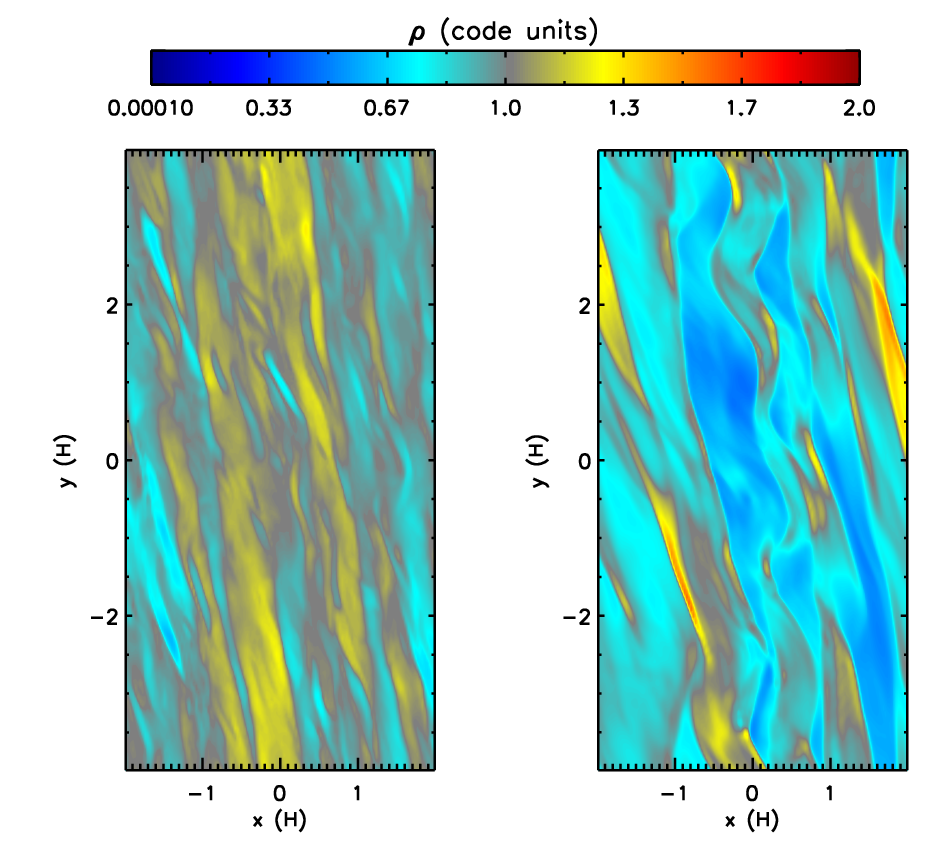
While we have established that we can force turbulence to roughly the same kinetic energy amplitude as the MRI-driven cases, it is worth asking what the structure of the forced turbulence is. Do the forced turbulence runs resemble their forcing functions at late times, or does a different structure emerge? In Figure 2, we plot the density in the mid-plane of the Resistive-50AU run and the Hydro-HA run at 100 orbits into the evolution. The two runs are visually nearly indistinguishable, and even in the forced turbulence case, there exist spiral density waves that propagate through the domain. Indeed, the auto-correlation function for the gas density [18, 33] returns a density structure that is very similar between the two runs. This similarity may be a result of the choice of forcing function for the hydro calculations; if we had chosen some other forcing function, perhaps these density waves would not exist or would look different to the MRI case. However, [23] suggest that these waves can be generally produced by disk turbulence, not necessarily restricted to that which is MRI-driven. In this respect, our hydro calculations are a representation of potential forms of disk turbulence that produce these waves other than the MRI.
Figure 3 displays the density-weighted turbulent velocity distribution for several integration depths and shearing box domain sizes, all in the ideal MHD limit. The dashed lines are and the solid lines are . The most striking feature of these plots is the rapid increase in the velocity of the peak of the distribution as one moves higher in the disk. For (upper half of the disk) the distribution peaks at about 10% of the sound speed, but this velocity increases to about 50% of for . The width of the distributions is quite large; for the domain, there is a probability that lies between 0.1 and 1. There does not appear to be a strong difference between the and distributions, with the latter being slightly more sharply peaked and at a slightly higher than the former. This suggests that the inclination of the disk will only weakly play a role in the observed turbulent velocity. Finally, convergence of the peak velocity with domain size appears to have been attained for the domain; this suggests that all the essential physics involved in setting the magnitude of velocity fluctuations is captured by this intermediate-sized domain.


Another interesting feature to note is the non-negligible supersonic velocity component to the distribution above . Integrating over the distribution for yields roughly 10% of the turbulent velocity being supersonic for box sizes larger than . The smaller domains have smaller supersonic components: and for the and , respectively. The origin of these supersonic velocities is presumably the steepening of initially subsonic waves as the density decreases away from the mid-plane. Similar physical effects have been seen in many prior simulations of stratified disks [42, 12, 6]. Along with the recently studied dissipation of current sheets in disk corona [25], shock heating from these supersonic motions could potentially play an important role in the thermodynamic properties of disk atmospheres. We will further explore these thermodynamic issues in future publications. We include the peak of the distribution and the percentage of the distribution with supersonic velocities for in Table 1.


In Figure 4 we plot the same velocity distributions for non-ideal (resistive) shearing boxes computed at different radial locations. Since the simulation conducted at 10 AU is highly variable, we show results that correspond both to the high stress turbulent state, and to the low stress state. Considering first the shearing box centered on 4 AU, it appears that as one probes regions closer to the mid-plane, the turbulent velocity fluctuations drop dramatically, with a peak in the distribution at . This is not surprising since the dead zone in this run extends to about , and the velocity fluctuations induced by the active layers appear within the dead zone region [10, 37, e.g.,]. Above the velocity distribution is very similar to the ideal MHD cases, including the presence of supersonic velocities.
Moving outward to near the outer edge of the dead zone, the 10 AU simulation yields a velocity distribution that varies slightly, depending on whether or not the system is in the “high state” or the “low state”. The low state appears to be intermediate in the velocity distribution between the 4 AU and ideal MHD cases, whereas the high state resembles the ideal MHD distribution more closely. In both states, the velocity distribution near the disk surface peaks around with a substantial supersonic tail, again agreeing with the other simulations. Finally, the shearing box centered on 50 AU has a distribution very similar to the ideal MHD case, consistent with the notion that the resistivity is small enough at this radius to not significantly affect the MRI.


Figure 5 displays the velocity distributions for the two forced hydro runs. Hydro-HA has a distribution quite similar to those in the MRI calculations. However, there is a weaker dependence of the turbulent velocity on the height from the mid-plane; the peak values lie between 0.2 and 0.5. Again, the peaks of the and distributions are quite similar. There is also a significant supersonic component to the distribution; 7-8% of the distribution has . The distribution peaks for Hydro-LA are lower, which is not surprising since there is less kinetic energy in this run. However, despite an order of magnitude difference in the saturated kinetic energies, the peak velocity for is only a factor of 2.5 lower in Hydro-LA than in Hydro-HA. The mid-plane velocities are significantly lower in Hydro-LA than in Hydro-HA, however. These results suggest that even when forced with a lower amplitude, the turbulent velocities can steepen significantly in the lower density regions away from the mid-plane. Taken together, the characteristic velocities in the forced hydro runs are not very different than those in the MRI cases.
V. Discussion and Implications for Observations


This paper represents a step toward making a direct connection between the simulated properties of turbulent protoplanetary disks and actual observations of these systems. To this end, we have presented a series of calculations with varying physics from which we extracted the turbulent velocity distribution. The simulations do not explicitly predict actual observables, as that would require the inclusion of radiation physics in one form or another. However, our results do have several implications for the nature of disk turbulence in low mass protoplanetary disks that could potentially be tested with future observations, particularly those made with ALMA.
The first implication is that if turbulence is driven solely by the MRI, the turbulent linewidth ought to vary strongly as a function of both radius and height above the mid-plane. In regions of the disk where non-ideal effects are small, we predict mid-plane velocities that peak near 0.1 times the local sound speed. The characteristic turbulent velocities increase with height, such that significant regions of transonic flow occur in the atmosphere at . This prediction is in at least rough agreement with the observational measurement of turbulent broadening in HD 163296, where [28] infer turbulent line widths consistent with a few tenths of the sound speed. The observational results for this system are then consistent with MRI-driven turbulence actually occurring in the outer disk. The upper limit for TW Hya, on the other hand, is at best marginally consistent with the MRI prediction for near-ideal conditions – pushing that limit lower has the potential to provide a stringent test of our models.
If we assume, on theoretical grounds, that the MRI is the only viable source of turbulence in low mass disks, then the agreement between our simulations and the observational results for HD 163296 is mildly encouraging. That is, MRI-driven turbulence produces the “right” answer. This order of magnitude level of agreement, however, is nowhere near discriminating enough to exclude the possibility that some (unspecified) hydrodynamic instability is responsible for the observed turbulent broadening. We have run purely hydrodynamic disk models that are driven to a turbulent state via large scale forcing, and these disks also show velocity fluctuations of the order of tenths of the sound speed, along with a velocity gradient between the mid-plane and the surface, where transonic velocities can be produced.
This raises the question, can observations distinguish between purely hydrodynamic turbulence and that driven by the MRI? Of course, one option is to observe the magnetic field structure and amplitude (or lack thereof) in the disk itself, but this is currently exceedingly difficult [27, but see]. If one cannot observe the field directly, the next best option is to observe a secondary effect of the magnetic field such as the turbulent velocity. However, as noted already, a single measurement of the turbulent velocity is certainly insufficient to distinguish between MHD and hydrodynamic drivers of turbulence. An arbitrary forcing of the fluid can still yield turbulent velocities that are more or less indistinguishable from those produced via the MRI.
The prospects for distinguishing between different sources of turbulence are better if observations are able to probe either different heights within the disk (by exploiting multiple molecular species), different radii, or both. In a real disk, of course, there is no immediately accessible observable that isolates the turbulence at a particular physical height above the mid-plane. Rather, the observable is the degree of broadening of a given molecular line produced in a region of the disk where the temperature, density and chemistry yield sufficient emissivity, and the optical depth is not too high. Thus, where in a particular line is emitted will depend on the vertical structure of the disk itself. We find that this structure differs significantly depending upon whether the disk is magnetized or not. Consider Fig. 6, which shows the time- and horizontally-averaged vertical density profile. The red curve is one of the forced hydro turbulence cases, and the other curves are a subset of the MRI-driven turbulence runs. There is an obvious and significant difference between the density profiles at large . The density departs significantly from Gaussian in the MRI cases. The reason for this is that for , magnetic pressure dominates over gas pressure, and the gradient in magnetic pressure helps to support the gas against gravity. Thus, the gas pressure and density have a shallower slope in these regions. This magnetic and gas pressure structure is consistent with previous shearing box simulations [24, e.g.,].
The difference in vertical structure between a magnetized and non-magnetized disk results in a distinct difference in the the profile of turbulent velocity with column density. This is shown in Figure 7, which plots how the characteristic turbulent velocity changes as a function of fractional column, defined as
| (18) |
where is the time- and horizontally averaged gas density (the time average is done from orbit 50 onwards). There are two features to note in this plot. The first is that, in general, the turbulent velocity decreases as one probes deeper into the disk. This result was discussed above in the context of the velocity distributions, and is simply the result of velocity steepening in lower density regions. The second feature is that the values obtained in the upper disk regions can be found at a lower (by about an order of magnitude) in the hydro case versus the MHD cases. This suggests that the column depth to which a particular line can probe may be very useful in determining the density structure away from the disk mid-plane and thus can constrain the turbulence mechanisms.
Furthermore, the radial dependence of the velocity gradient with distance from the mid-plane may also be useful. While the general trend of decreasing with height is robust in all of our calculations, the presence of the MRI dead zone dramatically changes this gradient. In particular, as Figure 7 shows (blue points), the presence of a magnetically dead zone is quite obvious as the turbulent velocities drop well below near the mid-plane region, but the active layers above and below the mid-plane, in combination with steepening, produce . Thus, if one were to probe different depths into the disk and find a dramatic decrease in turbulent velocity towards the mid-plane, this would be strongly indicative of a dead zone region.
VI. Conclusions and Uncertainties
Our conclusions about the turbulent properties of low mass protoplanetary disks are:
- 1.
Characteristic turbulent velocities are (0.1-1) for fully turbulent regions, in rough agreement with observations made to date [28, e.g.,]. These characteristic velocities are reasonably robust to variations in numerical (changes to local domain size) and physical (locations in a model disk) parameters.
- 2.
Turbulent velocity increases away from the disk mid-plane due to steepening. In the upper region of the disk (), the velocity distribution peaks around and has a significant () supersonic component. As one probes towards the mid-plane, is typical of fully turbulent disks.
- 3.
In calculations with an MRI dead zone near the mid-plane, the characteristic turbulent velocities are within the dead zone. In principle, with an improvement in sensitivity, observations that probe different depths could see the presence of the dead zone as velocities drop from 0.1-1 to .
- 4.
The density structure for is significantly different in the MRI versus purely hydrodynamic cases, which could have potential implications for the observed turbulent linewidths if different depths can be probed.
- 5.
The vertical and planar velocity distributions are quite similar, suggesting that turbulent linewidths will only weakly be dependent on the inclination angle.
Our predictions for the distribution of turbulent velocity in MRI-active disks suffer from a number of uncertainties. First, we have chosen to only focus on one non-ideal MHD effect, namely Ohmic resistivity. Other non-ideal effects – ambipolar diffusion and the Hall term – are also important in protoplanetary disks [29, 2, 46]. Ambipolar diffusion, in particular, is important in low density regions, and may affect the properties of turbulence in the most observationally accessible location – the disk atmosphere at large radius. Moreover, the resistivity that we have employed neglects dust physics. We also caution that some of the most striking qualitative trends that we observe are linked to the steepening of waves near the disk surface. Wave propagation in disks is known to depend upon the vertical thermal structure [5], and hence the isothermal structure that we have assumed may not always be adequate. Even before adding a treatment of the radiation physics, these limitations imply that there remains much work to be done to further constrain the turbulent velocities in simulations of MRI-active disks.
While our results coupled with recent observations provide mild support for the model of MRI-driven angular momentum transport, the calculations that we have presented here have not been able to identify a strong observational discriminant between MRI-driven and purely hydrodynamic turbulence. Quite precise measurements of the turbulence as a function of height will be needed to tell one from the other on purely observational grounds. In fact, if sufficiently high spatial resolution observations of the inner disk regions reveal the presence of a dead zone region, then this would present very strong support for the MRI driving disk turbulence.
Finally, we reiterate that we have considered only arbitrary hydrodynamic forcing, rather than setting up known physical drivers of turbulence, such as self-gravity or even convection [30]. By design, the average kinetic energy in the purely hydrodynamic simulations nearly equals that of the MRI simulations. If it could be established, theoretically, that hydrodynamic drivers of turbulence were necessarily weaker than the MRI, a single measurement of the turbulent velocity would then distinguish between the two. If, on the other hand, we treat the strength of hydrodynamic turbulence as a free parameter, then our results suggest that the vertical variation of turbulent velocities in the hydrodynamic and MHD limits can have a qualitatively similar trend. Of course, the physical mechanisms that might initiate hydrodynamic turbulence without arbitrary forcing could, in principle, imprint distinctive characteristics into the observable turbulent velocity field, which would allow them to be distinguished from the MRI more readily. To test this, it would be useful to repeat the analysis presented here for disks in which these other sources of turbulence are active. These calculations are currently underway and will be presented in future work.
References
- [1] Armitage, P. J. 2011, ARA&A, 49, 195
- [2] Bai, X.-N., & Stone, J. M. 2011, ApJ, submitted
- [3] Balbus, S. A., & Hawley, J. F. 1998, Reviews of Modern Physics, 70, 1
- [4] Bast, J. E., Brown, J. M., Herczeg, G. J., van Dishoeck, E. F., & Pontoppidan, K. M. 2011, A&A, 527, 119
- [5] Bate, M. R., Ogilvie, G. I., Lubow, S. H., & Pringle, J. E. 2002, MNRAS, 332, 575
- [6] Beckwith, K., Armitage, P. J., & Simon, J. B. 2011, MNRAS, 1130
- [7] Carr, J. S., Tokunaga, A. T., & Najita, J. 2004, ApJ, 603, 213
- [8] Chiang, E., & Youdin, A. N. 2010, Annual Review of Earth and Planetary Sciences, 38, 493
- [9] Davis, S. W., Stone, J. M., & Pessah, M. E. 2010, ApJ, 713, 52
- [10] Fleming, T., & Stone, J. M. 2003, ApJ, 585, 908
- [11] Fleming, T. P., Stone, J. M., & Hawley, J. F. 2000, ApJ, 530, 464
- [12] Flock, M., Dzyurkevich, N., Klahr, H., Turner, N. J., & Henning, Th. 2011, ApJ, 735, 122
- [13] Fromang, S., Terquem, C., & Balbus, S. A. 2002, MNRAS, 329, 18
- [14] Gammie, C. F. 1996, ApJ, 457, 355
- [15] Gardiner, T. A., & Stone, J. M. 2005, JCP, 205, 509
- [16] —. 2008, JCP, 227, 4123
- [17] Glassgold, A. E., Lucas, R., & Omont, A. 1986, A&A, 157, 35
- [18] Guan, X., Gammie, C. F., Simon, J. B., & Johnson, B. M. 2009, ApJ, 694, 1010
- [19] Haisch, Karl E., Jr., Lada, Elizabeth A., & Lada, Charles J. 2001, ApJ, 553, L153
- [20] Hartmann, L., Calvet, N., Gullbring, E., & D’Alessio, P. 1998, ApJ, 495, 385
- [21] Hawley, J. F., Gammie, C. F., & Balbus, S. A. 1995, ApJ, 440, 742
- [22] Hayashi, C. 1981, Progress of Theoretical Physics Supplement, 70, 35
- [23] Heinemann, T., & Papaloizou, J. C. B. 2009, MNRAS, 397, 52
- [24] Hirose, S., Krolik, J. H., & Stone, J. M. 2006, ApJ, 640, 901
- [25] Hirose, S., & Turner, N. J. 2011, ApJ, 732, L30
- [26] Hueso, R., & Guillot, T. 2005, A&A, 442, 703
- [27] Hughes, A. M., Wilner, D. J., Cho, J., Marrone, D. P., Lazarian, A., Andrews, S. M., & Rao, R. 2009, ApJ, 704, 1204
- [28] Hughes, A. M., Wilner, D. J., Andrews, S. M., Qi, C., & Hogerheijde, M. R. 2011, ApJ, 727, 85
- [29] Kunz, M. W., & Balbus, S. A. 2004, MNRAS, 348, 355
- [30] Lesur, G., & Ogilvie, G. I. 2010, MNRAS, 404, L64
- [31] Lubow, S. H., & Ida, S. 2010, in Exoplanets, ed. S. Seager. Tucson, AZ: University of Arizona Press, p. 347
- [32] Lynden-Bell, D., & Pringle, J. E. 1974, MNRAS, 168, 603
- [33] Nelson, R. P., & Gressel, O. 2010, MNRAS, 409, 639
- [34] Ormel, C. W., & Cuzzi, J. N. 2007, A&A, 466, 413
- [35] Sano, T., Miyama, S. M., Umebayashi, T., & Nakano, T. 2000, ApJ, 543, 486
- [36] Shakura, N. I., & Sunyaev, R. A. 1973, A&A, 24, 337
- [37] Simon, J. B., Hawley, J. F., & Beckwith, K. 2011, ApJ, 730, 94
- [38] Sorathia, K. A., Reynolds, C. S., Stone, J. M., & Beckwith, K. 2011, ApJ, submitted
- [39] Stepinski, T. F. 1992, Icarus, 97, 130
- [40] Stone, J. M., & Gardiner, T. A. 2010, ApJS, 189, 142
- [41] Stone, J. M., Gardiner, T. A., Teuben, P., Hawley, J. F., & Simon, J. B. 2008, ApJS, 178, 137
- [42] Stone, J. M., Hawley, J. F., Gammie, C. F., & Balbus, S. A. 1996, ApJ, 463, 656
- [43] Toro, E. F. 1999, Riemann Solvers and Numerical Methods for Fluid Dynamics (Berlin: Springer)
- [44] Turner, N. J., & Sano, T. 2008, ApJ, 679, L131
- [45] Wardle, M. 2007, Ap&SS, 311, 35
- [46] Wardle, M., & Salmeron, R. 2011, MNRAS, submitted
- [47] Williams, J. P., & Cieza, L. A. 2011, ARA&A, in press
- [48] Völk, H. J., Jones, F. C., Morfill, G. E., & Roeser, S. 1980, A&A, 85, 316