Performance Guarantee under Longest-Queue-First Schedule in Wireless Networks
Abstract
Efficient link scheduling in a wireless network is challenging. Typical optimal algorithms require solving an NP-hard sub-problem. To meet the challenge, one stream of research focuses on finding simpler sub-optimal algorithms that have low complexity but high efficiency in practice. In this paper, we study the performance guarantee of one such scheduling algorithm, the Longest-Queue-First (LQF) algorithm. It is known that the LQF algorithm achieves the full capacity region, , when the interference graph satisfies the so-called local pooling condition. For a general graph , LQF achieves (i.e., stabilizes) a part of the capacity region, , where is the overall local pooling factor of the interference graph and . It has been shown later that LQF achieves a larger rate region, , where is a diagonal matrix. The contribution of this paper is to describe three new achievable rate regions, which are larger than the previously-known regions. In particular, the new regions include all the extreme points of the capacity region and are not convex in general. We also discover a counter-intuitive phenomenon in which increasing the arrival rate may sometime help to stabilize the network. This phenomenon can be well explained using the theory developed in the paper.
Index Terms:
Wireless Networks Scheduling, Longest Queue First Policy, Stability, Local Pooling, InterferenceI Introduction
One of the long-standing challenges for wireless networks is how to utilize the communication medium efficiently when links interfere with each other. This paper is primarily concerned with an interference model called the protocol model, where two wireless links that interfere with each other are prohibited to transmit data simultaneously [1], [2], [3]. For the protocol model, a scheduling algorithm strives to select a set of non-interfering links for transmission in every time slot.
Finding efficient schedules can be very difficult. Tassiulas and Ephremides [4] showed that if the queue sizes for the links (which are nodes in the interference graph) are viewed as weights and a maximum weight independent set (MWIS) of the interference graph is selected as the schedule in each time slot, then the queues of the wireless network can be stabilized for any arrival rate vector inside the capacity region. However, finding an MWIS is NP-hard in general. Even under the more restricted -hop interference model, finding an MWIS is still NP-hard for [5, 3]. For the 1-hop interference model, the problem of finding an MWIS reduces to maximum weight matching and the complexity is , where is the number of wireless links [6]. Hence, scheduling using MWIS is inapplicable to large networks.
To reduce the complexity, some simple sub-optimal scheduling algorithms have been introduced [7, 8, 9, 10, 11, 12, 13]. The Longest Queue First (LQF, also known as the greedy maximal schedule) policy is recognized for its high performance in practice [6]. The LQF schedule chooses links in a decreasing order of the queue sizes while conforming to the interference constraints. Dimakis and Walrand showed that the LQF algorithm achieves (stabilizes) the entire interior of the capacity region, , when the interference graph satisfies the so-called overall local pooling condition [14]. For general cases, Joo et al. introduced a parameter called the overall local pooling factor, denoted by , where , based on the topology of the interference graph ; they showed the LQF algorithm achieves a subset of the capacity region, [6]. Several other authors studied how to check the local pooling condition or estimate for specific graphs [15, 16, 17].
A single-parameter performance characterization of LQF suggests a uniform rate reduction on the links. However, it is possible that the links are subject to heterogeneous interference relations and some links can perform better than others. To capture the performance heterogeneity, a multiple-parameter characterization of the stabilizable region by LQF was established in [18]. It was shown that LQF can achieve a larger rate region, , where is a diagonal matrix. Each diagonal entry of corresponds to a link and it summarizes the link’s interference constraints.
Even this multiple-parameter characterization of LQF underestimates the stability region. For instance, it excludes some parts of the capacity region that are obviously stabilizable by LQF. To progress further toward complete performance characterization, there is a need to go beyond the current framework of linear transformations on the capacity region. The goal of this study is to establish such a “non-linear” framework and expand our knowledge about the achievable rate region by LQF. The main contribution is to describe three new achievable rate regions (, and ), which are all larger than the previously-known regions. More precisely, we show that and . Furthermore, the closures of the new regions include all the extreme points of the capacity region and are not convex in general. This is in contrast to previously-known regions of stability, which are all convex and, in general, exclude some extreme points of the capacity region because they each are derived by reducing the capacity region through a linear transformation. We show that the new regions of stability (or their closures) are convex if and only if they are identical to the capacity region itself. The result implies that, when LQF cannot achieve the full capacity region, the largest achievable region, which is yet to be discovered, cannot be convex.
The characterization of the LQF performance has been substantially improved with these new stability regions. For instance, we have found that, for an arbitrarily large , there are cases where an arrival rate vector is outside all the previously-known stability regions but is in . In other words, the previously-known stability regions can underestimate the performance of LQF by an arbitrarily large factor in certain cases, whereas the new regions can avoid such poor estimates.
The study has also yielded an interesting, counter-intuitive finding that increasing the arrival rates may sometime help to stabilize the network. We have discovered an example where a rate vector achievable by LQF point-wise dominates another rate vector not achievable by LQF. It turns out the former vector is in the stability region whereas the latter is not.
We next summarize the key ideas of the paper. Our theory is developed based on considering the fluid limit of an unstable network. A typical scenario is that the maximum queue size has an overall trend to grow indefinitely, which requires that, at some time , a subset of the current longest queues continues to grow. From the set of the longest queues at time , there is a subset that grows at the fastest rate and remains the longest in the next infinitesimal time interval. Denote this subset by . Under LQF, the queues in will be served with priority in the next small time interval, which implies that the average service rate vector, when restricted to , comes from the convex hull of the maximal schedules with respect to . This convex hull is denoted by . For the queues in , the arrival rates must be larger than the service rates. The discussion motivates the definition of a strictly dominating vector for a queue set , which is a vector , when restricted to , strictly dominating at least one vector in . After removing the union of the strictly dominating vectors, where the union is over all possible subsets of the queues, we get .
Key to the development about is a refinement to the notion of strictly dominating vectors, which is called uniformly dominating vectors. For the aforementioned queue set , the arrival rates not only must be larger than the service rates, but also larger by the same amount, so that the queues in grow at the same rate. The removal of all the uniformly dominating vectors gives . Although the closure of contains , there is value in studying and reporting the results about both regions. First, the theory about provides building blocks for proving some of the results about . Second, appears to be well connected to the notion of local pooling in [14], thus, providing some continuity in the theoretical development, whereas does not appear so.
Throughout, we assume i.i.d. and mutually independent arrival processes. As Dimakis and Walrand pointed out, for the same average arrival rate vector, whether the arrival processes have zero or non-zero variances leads to significantly different stability behavior (the former is the case of deterministic arrivals with constant rates) [14]. They established a queue separation result for the case of non-zero variances and developed a rank condition that leads to queue separation. We generalize the rank condition. Then, we extend to a larger stability region for the case of non-zero variances. We also show the closures of and are the same.
Finally, we relate the problems of finding stability conditions under LQF to several problems in the fractional graph theory [19]. The latter provide tools for studying the stability regions introduced by the paper and for characterizing the set -local pooling factor given in [18].
The rest of the paper is organized as follows. In Section II, we specify the models and notations. In Sections III and IV, we introduce the and ( and ) regions, respectively. In Section V, we introduce the fractional coloring and related problems that are relevant to the study of the stability regions. In Section VI, we give some simulation results to confirm aspects of the theory. The conclusion is given in Section VII.
II Preliminaries
In our model, a wireless network is represented by an undirected interference (or conflict) graph , where the node set represents the set of physical, wireless links in the network and the edge set represents the interference relation among the physical links. Two nodes in are connected with an edge whenever the physical links they represent interfere with each other.11 1 All the graphs in this paper are interference graphs, unless specified otherwise. We assume the node set is arbitrarily indexed from 1 to , and hence, can be written as .
Given a subset of nodes , we denote to be the subgraph of induced by the nodes in . In other words, an edge belongs to if and only if and .
We assume a time-slotted system. The capacity of each wireless link is normalized to 1 per time slot. There is a queue associated with each wireless link at the transmitter. We assume single-hop traffic. Traffic arrives at the transmitter side of a link, joining the queue and waiting for transmission; after transmission, it leaves the network. We assume i.i.d. and mutually independent arrival processes to the queues. It is easy to see that, under the LQF schedule with either deterministic or typical random tie-breaking rules, the joint queue process is Markovian. By stability, we mean the Markov process is positive recurrent22 2 Without loss of generality, we assume the Markov Chain is irreducible. See [4] for general cases..
A schedule is denoted by a -dimensional 0-1 vector, where a value 1 in an entry indicates the corresponding link is active and 0 otherwise. A schedule is feasible if and only if the links that are active do not interfere with each other. A feasible schedule is said to be maximal if no additional links can be activated without violating the interference constraints. Therefore, every feasible schedule is an independent set of and every maximal schedule is a maximal independent set of .
For the graph , let denote the set of all the maximal schedules and let denote the convex hull of all the maximal schedules. When relevant, we also consider to be the matrix whose columns are all the maximal schedules, with arbitrary indexing of the schedules. Similarly, for a node-induced subgraph , let be the set (or matrix) representing all the maximal schedules of and let be the convex hull of all the maximal schedules in .
The capacity region of a network is defined as the set of arrival rate vectors that are supportable by time sharing of the feasible schedules. Equivalently,
| (1) |
For a non-empty subset of nodes , the capacity region is defined analogously by replacing with in (1) and is denoted by . In the above, means that vector is component-wise less than or equal to vector . The interior of the capacity region can be written as
| (2) |
The interior of the capacity region thus defined can be stabilized by the MWIS schedule and any rate vector outside the capacity region cannot be stabilized by any schedule [4].
Given a -dimensional vector , the -dimensional vector represents the restriction of to the set . That is, contains only those components of which correspond to the nodes in .
For a vector defined for a node set, let or denote the component associated with . Note that, if , then the notation indicates the th component of . However, if for some non-empty , then for , or is not necessarily the th component of . If is any other type of vector, denotes the th component of . We use to represent the vector . The dimension of the vector depends on the context.
The capacity region for the whole graph and the capacity region for the subset has the following relationship.
Lemma 1
An arrival rate vector if and only if for all non-empty , . Likewise, if and only if for all non-empty , .
Proof:
Suppose . Then, for some . It is easy to see that, for any non-empty subset , there must exist a vector such that . Then, . Hence, . The other direction is true by taking . The last statement of the lemma can be proved similarly. ∎
Throughout, in the statements about rate regions that involve topological concepts such as open/close sets and the interior of a set, the space is assumed to be the set of non-negative real vectors, i.e., . Also, in the set-complement operation for any rate region, the whole set is understood to be the non-negative real vectors. For a set , we let and denote the interior and complement of , respectively.
In the LQF schedule, the links with longer queues are activated at a higher priority than those with shorter queues, subject to the interference constraints. The following may be considered as a reference implementation of this schedule. First, one of the links with the longest queue is selected to be in the schedule; ties are broken with either an arbitrary deterministic rule or randomly. All links with which the selected link interferes are removed from further consideration. Then, the same selection process repeats over the remaining links yet to be considered until no links remain to be considered.
Remark: The following is the key mathematical property about LQF that is used throughout. Suppose, at time , a non-empty set dominates in the sense that, for any and any , the queue size of is greater than that of . Then, the schedule used at must be maximal when restricted to (i.e., with respect to ).
III Stability Region under LQF
In this section, we introduce a notion of strictly dominating vectors and construct a region denoted by based on this notion. The region is larger than and , which have previously been shown to be stabilizable by the LQF policy. Unlike those previously-discovered regions of stability, the region includes all the extreme points of and it is not convex in general.
III-A Review of Set, Link and Overall -local Pooling
Set -local pooling has been studied in [18]. It has many interesting properties and is related to (overall) -local pooling defined in [6].
Definition 1
Given a non-empty set of nodes , the set -local pooling factor for , denoted by , is given by
| (3) | ||||
| (4) |
It has been shown that the set -local pooling factor is equal to the optimal value of the following problem.
| (5) |
The link -local pooling factor is defined as follows.
Definition 2
The local pooling factor of a link , denoted by , is given by
| (6) | ||||
| (7) |
III-B Strictly Dominating Vectors and Region
We first discuss some intuition that leads to the construction of the region. When the network is unstable, a typical situation is that the size of the longest queues has an overall trend of increase, if one ignores the short-time fluctuations. This would not have occurred if, for any subset , the arrival rate is strictly less than the service rate at each node in . Here, we imagine is the set of nodes with the longest queues for an extended period of time. Then, over that period of time, the schedule on each time slot must be maximal when restricted to and, by time sharing of such maximal schedules, the (average) service rate must be in . The discussion motivates us to define the notion of strictly dominating vectors for a subset of the nodes.
Definition 3
Given a non-empty node set , a vector is a strictly dominating vector of if for some . The region composed with all the strictly dominating vectors of is called the strictly dominating region of and is denoted by . That is,
For convenience, if , we assume .
We are often interested in the complement of :
Definition 4
The region is defined by
Remark. A vector is outside if and only if for some non-empty node set . Also, when restricted to the components corresponding to the nodes in , is an open set (it is a union of open sets). Hence, is a closed set. It can also be helpful to think .
Lemma 2
Suppose an arrival rate vector satisfies . Then, for any non-empty subset and any , there exists such that , where is a constant independent of , and .
Proof:
Since , we have for some small enough . Suppose the conclusion of the lemma is not true. That is, suppose for any , there exists a non-empty subset and such that for all . We can choose satisfying . Then, . Hence, , which implies by Definition 4, leading to a contradiction. ∎
III-C Performance Guarantee of LQF in Region
Therorem 3
If an arrival rate vector satisfies , then, the network is stable under the LQF policy.
The full proof requires replicating most of the arguments in [14]. In the following, we only highlight the part of the argument that needs modification.
Proof:
Consider the fluid limit of the queue processes, denoted by for all . For a fixed (and regular) time instance , let be the set of those longest queues whose time derivatives at , , are the largest under a given LQF policy instance. The queues in will remain the longest with identical length in the next infinitesimally small time interval.
The service rate vector, when restricted to , must belong to the set . Roughly, this is because contains all the queues that are the longest and remain the longest in the near future, and hence, as remarked earlier, every LQF schedule being used must be a maximal schedule when restricted to .
Now imagine is the service rate vector for the nodes in at time t. Since , by Lemma 2, there exists a link such that for some constant . Then, . Hence, at any time instance, each of the longest queues decreases at a positive rate no less than . This is sufficient to conclude that the original queueing process is a positive recurrent Markov process (see [20]), which means the queues are stable. ∎
Next, we show contains the previously-known regions of stability for LQF.
Lemma 4
The following holds: .
III-D Shape of Region
The previously-known regions of stability under LQF, such as , are derived by reducing the capacity region through a linear transformation. Since the capacity region is convex, each of these derived stability regions is also convex. In contrast, we will show that the shape of the region is not convex in general. Furthermore, when the previously-known regions are not identical to , they exclude many, if not most, of the extreme points of . We will show that contains all the extreme points of .
Lemma 5
The set of all the independent sets of the interference graph , i.e., the set of all the feasible schedules, has a bijection to the set of all the extreme points of .
Note that we consider the empty schedule where no link is activated a trivial independent set. Lemma 5 establishes a connection between the graph topology and the geometry of in a vector space. The proof can be found in the Appendix.
Lemma 6
Suppose is a vector corresponding to an independent set of the interference graph . Then, .
Proof:
is an independent set of the node-induced subgraph for any non-empty . Then, for any , which implies . Since is arbitrary, we must have . ∎
Corollary 7
All the extreme points of the capacity region belong to .
Proof:

As an example, let be the six cycle graph in Fig. 1. The arrival rate vector corresponds to an independent set, and hence, . However, we know that . As a result, . The example shows that can be strictly larger than . In the example, contains not only the extreme points. For instance, one can check that, for , but .
The next example shows that, the previously-discovered stability regions and can underestimate the performance of LQF by an arbitrarily large factor in certain directions and in certain cases, whereas can avoid such poor estimates.
Lemma 8
For any , there exists an interference graph and an arrival rate vector such that , but .
Proof:
Consider the bipartite graph in Fig. 2 with pairs of nodes, where in this particular case. It is almost a complete bipartite graph except that every corresponding pair of nodes (such as nodes 1 and 2) does not have an edge between them. It is easy to check that . Therefore, the rate vector , where , is not in . For any , we can find a large enough and a small enough such that . Then, we have in . ∎


Though we cannot draw various regions in a high-dimensional vector space, it may still be helpful to make a highly simplified illustration with Fig. 3. The whole capacity region is convex. The region is derived by scaling down the capacity region using the diagonal matrix . This sort of scaling usually cuts off many or most extreme points of . The newly defined stability region is a superset of and contains all the extreme points of . The figure makes the point that is not convex in general. We next show is convex if and only if it is equal to .
Lemma 9
The following statements are equivalent.
1. is a convex.
2. is an overall local pooling graph.
3. .
Proof:
First, we prove that statement 1 implies statement 2. Suppose is not overall local pooling. We claim that there must exist a non-empty set and such that . Since is not overall local pooling, there exists a non-empty set such that , which implies that there exist and , according to (5). If , we have the required set , and with . If not, let . Because and , it is easy to show 33 3 Suppose we write , where each is a maximal schedule with respect to . We can represent as , where and for all . Since , we have for each . It is clear that corresponds to an independent set of , the subgraph of induced by . Moreover, by the maximality of with respect to , if for some , it must be that for some and and interfere with each other, i.e., . Therefore, must be maximal with respect to . Hence, by , we get .. Because and , there must exist such that . Then, . Thus, and . By renaming to be , to be and to be , we have the required set and with .
Let be an extended vector from such that and . According to Definition 3 and 4, . Since , we can write , where and for all , and for are all the maximal schedules with respect to . For each , let be a -dimensional vector extended from , such that when and when . Clearly, each corresponds to an independent set of . Hence, by Lemma 6, for all . Since and , we conclude that is not convex.
Next, we show that statement 2 implies statement 3. Since is an overall local pooling graph, (the identity matrix). By Lemma 4, . Hence, .
Finally, statement 3 implies statement 1 since is convex. ∎
Remark. Suppose, for a given interference graph, the LQF algorithm does not achieve the full interior of the capacity region. Lemma 9 implies that is not convex. Furthermore, since the closure of the full stability region of LQF (which is unknown) contains , it contains all the extreme points of the capacity region . Hence, the closure of the full stability region of LQF cannot be convex either, and it cannot be characterized by any linear transformation of the capacity region.
IV Stability Region under LQF
In this section, we develop a notion termed as uniformly dominating vectors. It leads to a stability region , which is a superset of . When the arrival processes are not constant, i.e., when the variances of the i.i.d. arrival processes are non-zero, we obtain a stability region , which contains .
IV-A Motivating Examples
Example 1: We will first give an example to show that an arrival rate vector can sometime be stabilized by LQF. Hence, there is a region larger than that captures the performance of LQF more precisely. The example also contains hints about how such a region can be defined.
Consider the six cycle graph in Fig. 1. There are exactly five maximal schedules: , , , , . Suppose the arrival rate vector is , where is some small enough constant. Let , and . Then, one can check that and , which implies that . For , . Hence, and by Definition 3 and 4.
Consider the fluid limit of the queue processes under LQF, denoted by , for all . For a fixed (regular) time instance , let be the set of those longest queues whose time derivatives at , , are the largest. The queues in will remain the longest with identical length in the next infinitesimally small time interval. Since , by Lemma 1. If , it is a fact that the node-induced subgraph satisfies the local pooling condition [18]. An argument similar to that in the proof of Theorem 3 shows that the queues in all have a negative drift.
The case of is more subtle. Since only the maximal schedules of are used during the aforementioned infinitesimally small time interval, we can assume that the service rate vector is , where and for all . In the fluid limit, for . By assumption, should be identical for all nodes . However, one can check that it is impossible to find such for the given . Therefore, the case of would not have occurred, and only the case of needs to be considered. Hence, is stable under LQF for the given , according to the discussion for the case.
Example 2: Let , , , , , and and . Both and are outside . Interestingly, although , cannot be stabilized by LQF while can. This has been verified by simulation experiments under constant arrivals. We will next develop a theory that provides a larger stability region and also can explain this counter-intuitive example.
IV-B Uniformly Dominating Vector and Region
Definition 5
Given a non-empty node set , a vector is said to be a uniformly dominating vector of if for some and scaler . The region composed with all the uniformly dominating vectors of is called the uniformly dominating region of and is denoted by . That is,
By convention, if , we assume .
Definition 6
The region is defined by
Remark. Note that a vector is outside if and only if for some non-empty node set .
Lemma 10
For any non-empty , is closed. Hence, is open.
Proof:
Let , where is dimensional, and let . It is easy to see is compact and is closed. From Definition 5, is extended to the -dimensional space. It can be shown that is closed, and hence, is closed. Then, is open (with respect to the metric space ). ∎
Lemma 11
Suppose and suppose is a non-empty node set. If for some , then , for some independent of and .
Proof:
Suppose (here, is of -dimension) for some . Since and is open, (here, is of -dimension) for some small enough independent of and . Then or . Since , . Hence, or . ∎
The constant will serve as a bound for the rate of the Lyapunov drift in the performance analysis.
IV-C Performance Guarantee of LQF in Region
Therorem 12
If an arrival rate vector satisfies , then, the network is stable under the LQF policy.
Proof:
Again, consider the fluid limit of the queue process and apply a similar argument as in the proof of Theorem 3. Let be the set of nodes whose queues are the longest at time and will remain the longest for the next infinitesimally small time interval. Let be the service rate vector for the nodes in at time . Under LQF, and for some . Since , by Lemma 11, we have for some independent of and . Hence, at any time instance, each of the longest queues decreases at a positive rate no less than . This is sufficient to conclude that the original queueing process is a positive recurrent Markov process, which means the queues are stable. ∎
Lemma 13
.
Proof:
Suppose . Then, there exists a vector and . Hence, for some non-empty , and . Since , for some small enough . From and , we have . Hence, , leading to a contradiction. ∎
IV-D Rank Condition and Region
For the same average arrival rate vector, whether the i.i.d. arrival processes have zero or non-zero variances leads to significantly different stability behavior (in the former case, the arrival processes are deterministic with constant rates). This issue has been discussed in [14] where the authors develop a queue separation result related to a rank condition about the matrices of the maximal independent sets. We next generalize the rank condition. Then, we extend to a larger stability region . We will show can be stabilized under LQF when the arrival processes all have non-zero variances.
Definition 7
Let be a non-empty set. We call the matrix the extended schedule matrix for (or graph ). Let denote the rank of the extended schedule matrix, i.e., the number of linearly independent columns in the matrix . We say (or graph ) has a high rank if . Otherwise, we say (or ) has a low rank.
Suppose is the set of nodes with the longest queues at some time instance. When the arrival has non-zero variances, the queue separation result suggests (Lemma 1 and Lemma 3 of [14]): If the rank , then, with probability 1, the queue sizes of will not stay identical in the next infinitesimal time interval. We find that the condition can be relaxed to , i.e., the low rank condition in Definition 7. The queue separation lemma (Lemma 1 of [14]) uses the assumption to obtain a vector such that and . Such a vector still exists when the low rank condition in Definition 7 is satisfied. Then, every subsequent step in the proof of the queue separation lemma still holds. The low rank condition is a generalization since implies .
Roughly speaking, when the variances are non-zero, the randomness in the arrival processes pressures the queues in to move around in an -dimensional space. This means that the queues cannot be simultaneously the longest queues for a sustained period of time (in which case, the queue trajectory moves along a line), unless the service can fully compensate the pressure from the arrival processes. But, full compensation is not possible in the low-rank case since the service rate vector lives in a lower-dimensional space. What will happen is that some subset of the queues in with a high rank will dominate the rest. This is known as queue separation. The implication is that, in the case of non-zero variances, there is no need to consider the low-rank subsets of when evaluating the performance degradation of LQF. The discussion motivates the following definition of .
Definition 8
The region is defined by
In words, a vector is outside if and only if for some node set that has a high rank.
By comparing the definitions of and , we have the following lemma.
Lemma 14
.
In addition to the i.i.d and mutually independent assumptions, the following assumption on the arrival processes is needed for technical reasons (see [14] for their relevance).
A1: (The large deviation bound on the arrival processes) Let be the cumulative arrivals at queue (at node ) up to time , and let be the average arrival rate at queue . For each ,
Therorem 15
Assume the condition in A1 holds and assume the variance of the i.i.d arrival process to each node is non-zero but finite. If an arrival rate vector satisfies , then, the network is stable under the LQF policy.
Proof:
Again, consider the fluid limit of the queue process and apply a similar argument as in the proof of Theorem 3. Let be the set of nodes whose queues are the longest at time and will remain the longest for the next infinitesimally small time interval. By replicating most of the arguments in the queue separation lemmas (Lemma 1 and Lemma 3 in [14]), it can be shown that must have a high rank44 4 The only change is to Lemma 3 in [14]. Instead of saying for any low-rank set, there must be a subset that satisfies local pooling, we say for any low-rank set, there must be a subset that is of high rank. This is so because a set with a single node is of high rank. The modification is needed in the proof of Lemma 3 in [14]. The statement of Lemma 3 also needs to be modified accordingly.. Otherwise, the queue sizes of the nodes in will be separated and they cannot all remain the longest. Hence, we can apply the same argument as that in Theorem 12, but only to the high-rank node sets. ∎
Some graph examples are given in Fig. 4, regarding their set -local pooling factors and ranks. Note that, the shaded region includes those subsets which either satisfy , i.e., set local pooling (SLoP), or have low rank. Those subsets need not to be considered for the performance of LQF in case of non-zero variances.

IV-E Further Properties of Regions and
It has been demonstrated that . We now continue to study the properties of the two regions and their relationship.
Therorem 16
The closures of and are the same, i.e. .
Proof:
Since , we have . We will next show . Since and , we only need to show .
Given any vector , by comparing Definition 6 and 8, we have
By Lemma 10, is a closed set and is open. Hence, is open. Therefore, there exists such that whenever and the distance between the two vectors .
Let and . Then, the distance between and is . Then, and .
Now, let . We will next construct a sequence of low-rank node sets, , for . Since each of them has a low rank, there exists an -dimensional vector with such that and . We then extend each to a -dimensional vector by setting the values of the new components to be zero. With a little abuse of notation, we call this -dimensional vector as well.
We now construct the sequence of . If , pick any subset . Let . Next, if , pick any and let . In step , if , we will pick any and let . This procedure will go on until becomes empty for some . We can check that the th component of is . This ensures that is always a non-negative vector for all .
Now, we will show that there exists an integer such that becomes empty for the first time (hence, the sequence of ends at , or contains no elements if ). For convenience, let .
We will show that for , where . Suppose for some . Then, , which implies that for some and . From the construction procedure, we know that , which implies that for some and . Since
we have
Then,
However, since , we have , leading to a contradiction. Hence, for .
In summary, each non-empty in the constructed sequence is in but not in for . Hence, each is distinct. Since there is a finite number of non-empty node sets , there exists an integer such that becomes empty for the first time.
Then, for any node set with a low rank. Hence, . The distance between and is . Then, the distance between and is . Hence, . It follows .
Since can be chosen arbitrarily small, is a limit point of . Thus, , implying . Hence, . ∎
The following is an intermediary lemma.
Lemma 17
If a non-empty set satisfies , then .
Proof:
Suppose there exists a vector . By Definition 5, for some and . Since , by Lemma 1, for some and a small enough . Hence, . Thus, and we arrive at a contradiction. ∎
Lemma 18
If every high-rank node set satisfies , then, and .
Proof:
According to Definition 8, we have . For any high-rank node set , since , we have by Lemma 17, which implies . Hence, . Combining this with Theorem 16, we get . Also, the fact that implies . Since is an open set in and is the largest open set in , it must be that . ∎
Remark. From Lemma 18, we know that when all the subsets satisfy either set local pooling (i.e., ) or the rank of is low, then . That is, the entire is achievable by LQF, assuming the arrival processes have non-zero variances. This is the same statement as Theorem 1 of [14]. Thus, the newly developed theory here is able to reproduce the main result of [14].
Lemma 19
if and only if is convex. Similarly, if and only if is convex.
Proof:
It is obvious that implies is convex. We will next show the converse. Since and is a closed set, we have . Because , we have . Since contains all the extreme points of (Corollary 7), also contains all of them. Since is the convex combination of all its extreme points and is convex, we must have .
The second statement can be proved similarly. ∎
V Graph coloring and LQF scheduling
The scheduling problem in this paper is deeply connected with graph coloring and its related problems. In this section, we will introduce fractional coloring, and more generally, aspects of the fractional graph theory that can provide useful tools for studying the stability regions discussed in the previous sections.
V-A Fractional Coloring and Capacity Region
The chromatic number of a graph , denoted by , is the minimum number of colors needed to paint the nodes so that the connected nodes do not share the same color. When we relax the integrality constraints of the chromatic number problem and introduce a parameter , we obtain the following linear programming (LP) problem.
Definition 9
Given a graph and , the weighted fractional coloring problem with the weight vector is:
| (9) |
The optimal value of the above problem, , is called the weighted fractional chromatic number, which is known to be related to the capacity region as follows (see [21]):
| (10) |
Based on (9), can be interpreted as the fastest way of serving queued data when the queue sizes are proportional to the weights . Based on (10), can be interpreted as the ‘traffic load’ to the network.
The relevance and usefulness of this problem to the study of wireless scheduling have been amply demonstrated in [21]. The characterization of the capacity region by (10) suggests that the fractional chromatic number can serve as an oracle for judging whether an arrival rate vector is in the capacity region or not. With this observation and with known complexity results about the fractional coloring problem, the authors of [21] have derived results about the inherent complexity of the wireless scheduling problem.
V-B Weighted Fractional Matching Number and Region
We next discuss the problem of finding the weighted fractional matching number of a graph [19]. This problem can help to decide whether a vector is in .
Definition 10
Given a graph and , the weighted fractional matching number problem with the weight vector is:
| (11) |
The above problem is the Lagrangian dual of the weighted fractional transversal number problem, which is the hypergraph dual problem of the weighted fractional coloring problem [19]. Here, the th component of can be interpreted as the amount of time for which the th maximal schedule is used. The weighted fractional matching number, , can be interpreted as the slowest way of serving the queued data (in the amount ) using only the maximal schedules, subject to the additional constraint that a schedule should not be selected if it activates a link associated with an empty queue.
Lemma 20
The region satisfies the following:
Proof:
Consider any vector and an arbitrary non-empty node set . Suppose . Then, by Definition 10, we have for some and . Let be the largest subset in such that . Note that . Then, the vector and . Hence, , which implies that . According to Definition 3 and 4, .
Conversely, suppose a vector satisfies for every non-empty . Then, for any . Otherwise, there would exist such that for some , which implies that . Thus, . ∎
V-C Hypergraph Duality and Set -local Pooling
We next relate the ratio of and to the set -local pooling factor. First, we have the following lemma.
Lemma 21
For any , and .
Proof:
The case of is trivial. We only focus on the case of . Suppose is an optimal solution to the problem in (11) for finding . Then, is feasible to the problem for finding . Since , .
Conversely, suppose is an optimal solution to the problem for finding . Then, is feasible to the problem for finding . Since , . Therefore, , for . A similar argument can be used to show . ∎
Therorem 22
Given a non-empty node set , the set -local pooling factor of satisfies the following55 5 We take the convention for any scalar . Note that, if any component of is equal to zero, then . As a result, the optimal solution to (12) must satisfy .:
| (12) |
Proof:
Suppose is an optimal solution to the problem in (5). Then, we choose . Since , we have
The last inequality above uses the fact , which follows from (10) (since ).
Because , there exists a non-negative vector such that and . Such is feasible to (11) for finding . Hence, . Therefore, .
Next, suppose is an optimal solution for the problem . Suppose and are optimal solutions for the problems of finding and , respectively. Then, we have . Now, let and . Then, and
By the feasibility of and to (9) and (11), respectively, . Hence,
Thus, is feasible to the problem in (5). Therefore, . ∎
The theorem above shows that the set -local pooling factor is the same as the minimum of the hypergraph duality ratios over all different weights.
V-D Weighted Fractional Domination Number and Region
Definition 11
Given a graph and , the weighted fractional domination number problem with the weight vector is:
For convenience, let when the problem is infeasible.
Lemma 23
The following relations hold:
VI Experimental Examples
In this section, we show some simulation results. The main purpose is to confirm some of the less intuitive theoretical results. We first show the performance of LQF on the six-cycle graph, denoted by , for arrival rate vectors in different sections of the capacity region. For , LQF can achieve the entire interior of the capacity region for arrivals satisfying assumption A1 and with non-zero variances. On the other hand, for constant arrivals, experiments have shown that some rate vectors in the interior of the capacity region are not achievable by LQF.
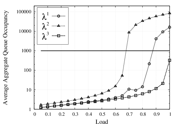
In the experiments with constant arrivals, we use a load parameter to scale the arrival rate vectors. Each experiment runs for iterations with initial queue sizes of . The following arrival rate vectors are used for the results in Fig. 5:
where . Note that . However, judging by the queue sizes in Fig. 5, the arrival rate vectors and seem to be not stabilizable, whereas seems to be stabilizable. The theory allows this counter-intuitive phenomenon. Readers can verify that while .
In Section IV, we generalize the definitions of high or low-rank graphs. In Fig. 6, we provide an interference graph that is not set local pooling () and is of high rank according to the original definition in [14]. However, in the new definition, the graph is of low rank. We ran simulations with initial queue sizes of using the Bernoulli arrivals with an identical arrival rate of 0.499. Fig. 7 shows the evolution of the average queue size for nodes 1-8 and 9-13 over iterations. The queues for nodes 1-8 appear to be unstable and the queues for nodes 9-13 appear to be stable. Our refinement of the rank condition rules out the possibility that the queues of all nodes are simultaneously the longest and remain longest, whereas the previous rank condition does not rule that out.


VII Conclusion
In this paper, we investigate the performance guarantee of the LQF scheduling policy in wireless networks. The objective is to discover new stability regions of LQF that are larger than those previously known, and to improve our knowledge about the largest possible stability region of LQF. We show that it is necessary to go beyond the existing framework of linear reduction of the capacity region, and move to a non-linear framework.
We introduce the concepts of strictly dominating vectors and uniformly dominating vectors; the former leads to the new stability region of LQF, , and the latter leads the stability regions and . We show that contains , which is the stability region given in [18]. We also show . Hence, the new stability regions all capture the performance of LQF better. Contrary to the previously-known regions of stability, the closures of these new stability regions contain all the extreme points of the capacity region , but they are not convex in general. The only case where they are convex is when they are equal to the capacity region itself, which occurs only for selected interference graphs. The general lack of convexity is not a defect of the theory. We show that, when LQF cannot achieve the full capacity region, the largest achievable region cannot be convex.
The study reveals a counter-intuitive situation where increasing the arrival rates helps LQF to stabilize the network. It turns out, in this case, the original rate vector is outside , and after the rate increase, the new rate vector is inside . We also generalize the rank condition studied in [14], and with this generalization, refine the stability results for non-deterministic arrivals. We can show that if a set of nodes satisfies the new low-rank condition, the queue sizes of these nodes will be separated. Based on this result, we can enlarge to , which is achievable by LQF under non-deterministic arrivals. Interestingly, we show that the closures of and are the same. Finally, we introduce several linear programming problems encountered in the fractional graph theory, which can provide tools for studying the newly developed stability regions. We show that a ratio between the weighted fractional coloring number and the weighted fractional matching number is related to the set -local pooling factor introduced in [18].
VIII Appendix
Proof:
Suppose is an independent set of , represented by a 0-1 vector. Clearly, . Let us write for some , and . Note that for every . Thus, and . For any index , if , we must have and . Similarly, if , we have . Therefore, and is an extreme point of .
Conversely, take any extreme point of . Then, for some . For an index , if , we claim that . Otherwise, we let . Then, we can create and such that for . We can find an such that , and we let . Since , we have . It is easy to see , which implies is not an extreme point. Hence, either or , for all .
We now show that or for all . Write as , where each , each , and . Let if ; otherwise, for all . Because , we have or . It is easy to check that . Since , we have for each . Since is an extreme point of , . Thus, or for all .
It is easy to see that any 0-1 vector in must be a feasible schedule, i.e., an independent set of . Since , the set of nodes, , for which forms an independent set. Let be the set of nodes for which . We have . Therefore, corresponds to an independent set. ∎
References
- [1] X. Lin, N. B. Shroff, and R. Srikant, “The impact of imperfect scheduling on cross-layer rate control in wireless networks,” IEEE/ACM Transactions on Networking, vol. 14, no. 2, pp. 302–315, April 2006.
- [2] H. Balakrishnan, C. Barrett, V. Kumar, M. Marathe, and S. Thite, “The distance-2 matching problem and its relationship to the MAC-layer capacity of ad hoc networks,” IEEE Journal on Selected Areas in Communications, vol. 22, no. 6, pp. 1069–1079, 2004.
- [3] G. Sharma, R. R. Mazumdar, and N. B. Shroff, “On the complexity of scheduling in wireless networks,” in Proccedings of ACM MobiCom, 2006, pp. 227–238.
- [4] L. Tassiulas and A. Ephremides, “Stability properties of constrained queueing systems and scheduling policies for maximum throughput in multihop radio networks,” IEEE Transactions on Automatic Control, vol. 37, no. 12, pp. 1936–1948, Dec 1992.
- [5] G. Sharma, N. B. Shroff, and R. R. Mazumdar, “Maximum weighted matching with interference constraints,” in PERCOMW ’06: Proceedings of the 4th annual IEEE international conference on Pervasive Computing and Communications Workshops, 2006.
- [6] C. Joo, X. Lin, and N. B. Shroff, “Understanding the capacity region of the greedy scheduling algorithm in multi-hop wireless networks,” in Proceedings of IEEE INFOCOM, 2008.
- [7] L. Chen, S. H. Low, M. Chiang, and J. C. Doyle, “Cross-layer congestion control, routing and scheduling design in ad hoc wireless networks,” in Proceedings of IEEE INFOCOM, April 2006.
- [8] A. Gupta, X. Lin, and R. Srikant, “Low-complexity distributed scheduling algorithms for wireless networks,” in Proceedings of IEEE INFOCOM, May 2007.
- [9] C. Joo and N. Shroff, “Performance of random access scheduling schemes in multi-hop wireless networks,” in Proceedings of IEEE INFOCOM, 2007.
- [10] X. Lin and S. B. Rasool, “Constant-time distributed scheduling policies for ad hoc wireless networks,” in Proceedings of the IEEE CDC, 2006.
- [11] E. Modiano, D. Shah, and G. Zussman, “Maximizing throughput in wireless networks via gossiping,” ACM SIGMETRICS Performance Evaluation Review, vol. 34, no. 1, pp. 27–38, 2006.
- [12] S. Sanghavi, L. Bui, and R. Srikant, “Distributed link scheduling with constant overhead,” ACM SIGMETRICS Performance Evaluation Review, vol. 35, no. 1, pp. 313–324, 2007.
- [13] P. Chaporkar, K. Kar, and S. Sarkar, “Throughput guarantees through maximal scheduling in wireless networks,” in Proceedings of 43d Annual Allerton Conference on Communication, Control and Computing, 2005, pp. 28–30.
- [14] A. Dimakis and J. Walrand, “Sufficient conditions for stability of longest-queue-first scheduling: Second-order properties using fluid limits,” Advances in Applied Probability, vol. 38, pp. 505–521, 2006.
- [15] M. Leconte, J. Ni, and R. Srikant, “Improved bounds on the throughput efficiency of greedy maximal scheduling in wireless networks,” in Proceedings of MobiHoc, 2009.
- [16] B. Birand, M. Chudnovsky, B. Ries, P. Seymour, G. Zussman, and Y. Zwols, “Analyzing the performance of greedy maximal scheduling via local pooling and graph theory,” Columbia University, Tech. Rep., July 2009. [Online]. Available: http://www.columbia.edu/~bb2408//pdfs/AnalyzingGMS.pdf
- [17] M. C. B. Ries and Y. Zwols, “Claw-free graphs with strongly perfect complements. fractional and integral version.” Columbia University, Tech. Rep., Jan 2010. [Online]. Available: http://www.columbia.edu/~yz2198/papers/clawfree1.pdf
- [18] B. Li, C. Boyaci, and Y. Xia, “A refined performance characterization of longest-queue-first policy in wireless networks,” in Proceedings of MobiHoc ’09, New Orleans, LA, USA, 2009, pp. 65–74, also accepted to IEEE/ACM Transactions on Networking.
- [19] E. R. Scheinerman and D. H. Ullman, Fractional Graph Theory: A Rational Approach to the Theory of Graphs. New York, USA: John Wiley & Sons Inc., 1997.
- [20] J. G. Dai, “On positive Harris recurrence of multiclass queueing networks: A unified approach via fluid limit models,” Annals of Applied Probability, vol. 5, pp. 49–77, 1995.
- [21] C. Boyaci, B. Li, and Y. Xia, “An investigation on the nature of wireless scheduling,” in Proceedings of IEEE INFOCOM, March 2010.