跳到论文正文
W Papers独立论文阅读器 arXiv:1107.2707 论文正文 计算阅读时间 · 0%
引用这篇论文根据当前论文元数据生成,正式投稿前建议核对。


License: arXiv.org perpetual non-exclusive license
arXiv:1107.2707v2 [quant-ph] 18 Jul 2013

Structure of 2D Topological Stabilizer Codes

Héctor Bombín Affiliation: Perimeter Institute for Theoretical Physics
31 Caroline St. N., Waterloo, ON, N2L 2Y5, Canada
Abstract

We provide a detailed study of the general structure of translationally invariant two-dimensional topological stabilizer quantum error correcting codes, including subsystem codes. We show that they can be understood in terms of the homology of string operators that carry a certain topological charge. In subsystem codes two dual kinds of charges appear. We prove that two non-chiral codes are equivalent under local transformations iff if they have isomorphic topological charges. Our approach emphasizes local properties over global ones.

1 Introduction

Quantum error correcting codes [1, 2, 3, 4] play a fundamental role in the quest to overcome the decoherence of quantum systems. Among them, stabilizer codes [5, 6] provide a large and flexible class of codes that are at the same time relatively easy to investigate. Interactions between physical qubits are sometimes subject to locality constraints in a geometrical sense. E.g., qubits might be placed in a DD-dimensional array with interactions available only between nearest neighbors. In such cases the subclass of topological stabilizer codes (TSC) [7, 8, 9, 10, 11, 12, 13, 14] is a natural choice. TSCs not only have very nice locality properties, but are also flexible in terms of the manipulation strategies that they allow.

The purpose of this paper is to investigate the general structure of two-dimensional TSCs, covering both subspace codes and the more general subsystem codes [15, 16, 17]. The only constraint imposed is translational symmetry of the bulk of the code, which provides a way to list the codes.

A stabilizer quantum error correcting code is described in terms of certain ‘check operators’, a set of commuting observables that have to be measured in order to get information about what errors have affected an encoded state. In TSCs these measurements are local in a geometrical sense. In particular, a TSC is in practice usually given as a recipe to construct the check operators on a given lattice of qubits. The lattice can be arbitrarily large, but check operators are defined locally, with support on a set of qubits contained in a bounded region. What makes these codes topological, as opposed to simply local, is that no information about the encoded qubits can be recovered if only access to a local set of qubits is granted. Indeed, operators on encoded qubits have support on a number of physical qubits that grows with the lattice size.

An essential feature of known topological codes is that they have an error threshold [8, 18, 19, 20, 21]. I.e., in the limit of large lattices, for noise below a certain threshold error correction is asymptotically perfect. This is true either in a simple error correction scenario or in a fault-tolerant scenario, and also when qubit losses are taken into account [22]. It is also often true [23] —but for interesting exceptions, see[12, 14]— that the number of encoded qubits depends only on the homology of the qubit lattice. In particular a trivial homology gives no encoded qubits, but even in a planar setting it is possible to recover non-trivial codes by introducing suitable boundaries [24] and other defects such as twists [25]. Moreover, because in such ‘homological’ codes the lattices can be chosen very flexibly, it is possible to carry out certain computations by changing the code geometry over time, something called ‘code deformation’ [8, 26, 27]. Error correction turns out to be connected to classical statistical models [8, 19, 11] and this has given rise to fast algorithms to infer the errors [28]. Finally, there exist topological codes that are especially well suited to perform computations using transversal gates [9, 10], which minimizes error propagation.

General properties of TSCs in two or higher dimensions have already been explored to different degrees. General constraints on the code distance —directly related to the geometry of encoded operators— were first found in [29], and improved in [30]. The subsystem case was addresed in [31]. The geometry of logical operators in a subclass of TSCs, subject to constraints such as scale invariance of the number of encoded qubits, was studied in [23]. Constraints on the code distance for three-dimensional codes that do not satisfy this scale invariance condition have been recently developed [32].

One of the main results in this paper is that all two-dimensional TSCs can be understood in terms of ‘string operators’ that carry a ‘topological charge’. In particular, homology plays an essential role and dictates the number of encoded qubits. In the case of subspace codes, the corresponding Hamiltonian model [7] —which has the code as its gapped ground state— exhibits anyonic excitations. Moreover, all subspace codes that give rise to the same anyon model turn out to be equivalent, in the sense that there exists a local transformation connecting them. The implications of this result, both from the condensed matter and quantum information perspectives, are explored in [33]. In the case of subsystem codes we no longer have a direct interpretation in terms of physical anyons. However, we find a nice duality structure between two kinds of charges. The first kind corresponds to an anyon model —possibly chiral—, and the second to fluxes with which the anyons interact topologically. We show that codes giving rise to the same non-chiral anyon model are locally equivalent. Computational implications of these results are discussed in the conclusions.

Our approach emphasizes local properties of the codes —such as the structure of check operators— over global ones —such as the number of encoded qubits. In practice we realize this by considering infinite versions of the codes that cover the plane. The idea is that all operators acting on a finite number of qubits become automatically local in this infinite picture. At the same time, the homology of the plane is trivial and this simplifies the analysis.

The paper is divided as follows. Section 2 informally summarizes the main results, providing the intuition behind the main definitions and proofs. Section 3 introduces in a formal manner topological stabilizer groups (TSGs), used to model TSCs. Subsequent sections develop diverse aspects of the structure of TSGs, culminating in a structure theorem in section 8 that we use to prove local equivalence. Finally, section 9 discusses natural extensions of this work.

To avoid repetition, we will often omit the qualifier “two-dimensional” when discussing lattices, TSCs, and so on, but it should be understood in all cases.

2 Approach and results

The purpose of this section is to summarize informally the approach taken to investigate TSCs and the results obtained. At the same time, it explains the motivation behind the main definitions and the intuition behind some proofs.

2.1 Stabilizer codes

Given a system with nn qubits, its Pauli group is

𝒫n:=⟨i​𝟏,X1,Z1,…,Xn,Zn⟩,\mathcal{P}_{n}:=\langle i\mathbf{1},X_{1},Z_{1},\dots,X_{n},Z_{n}\rangle, (1)

where XiX_{i}, ZiZ_{i} denote the Pauli XX and ZZ operators acting on the ii-th qubit. A stabilizer code [5, 6] on nn qubits is defined by a subgroup of Pauli operators 𝒮⊂𝒫\mathcal{S}\subset\mathcal{P}, called stabilizer group, such that −1∉𝒮.-1\not\in\mathcal{S}. 𝒮\mathcal{S} is then abelian and its elements are self-adjoint. The code is composed by those states |ψ⟩∈𝐂2n|\psi\rangle\in\mathbf{C}^{2^{n}} such that s​|ψ⟩=|ψ⟩s|\psi\rangle=|\psi\rangle for every stabilizer s∈𝒮s\in\mathcal{S}. It is enough to check these conditions for a set {si}\{s_{i}\} of independent generators of 𝒮\mathcal{S}. Such stabilizer generators serve as check operators: they can be measured in order to recover information about any errors affecting the encoded states. If 𝒮\mathcal{S} has n−kn-k independent generators the code subspace has dimension 2k2^{k}, it encodes kk logical qubits. The logical or encoded Pauli operators are recovered as the quotient

𝒵𝒫n​(𝒮)𝒮≃𝒫k,\frac{\mathcal{Z}_{\mathcal{P}_{n}}({\mathcal{S}})}{\mathcal{S}}\simeq\mathcal{P}_{k}, (2)

where 𝒵𝒫n​(𝒮)\mathcal{Z}_{\mathcal{P}_{n}}({\mathcal{S}}) denotes the centralizer of 𝒮\mathcal{S} in 𝒫n\mathcal{P}_{n}. This centralizer is the group of undetectable Pauli errors: those that do not change the error syndrome. The quotient is necessary because the elements of 𝒮\mathcal{S} are trivial undetectable errors, without any effect on encoded states.

Given a set {si}\{s_{i}\} of generators of 𝒮\mathcal{S} we can write down a Hamiltonian H=−∑isi.H=-\sum_{i}s_{i}. Its ground subspace is the code subspace, and there is a gap of two energy units to any excited state. This gap is important when we consider families of TSCs with local generators in systems of arbitrary size, because the size independence of the gap gives rise to a gapped phase. An error syndrome in the code amounts to an excitation configuration in the Hamiltonian system.

It is also possible to encode only in a subsystem of the code subspace. In the stabilizer formalism this logical subsystem can be described as that in which the action of a certain gauge group 𝒢⊂𝒫\mathcal{G}\subset\mathcal{P} is trivial [16]. The gauge group satisfies

𝒵𝒢​(𝒢)∝𝒮\mathcal{Z}_{\mathcal{G}}({\mathcal{G}})\propto\mathcal{S} (3)

and we assume ⟨i​𝟏⟩⊂𝒢\langle i\mathbf{1}\rangle\subset\mathcal{G}. Logical operators are recovered from

𝒵𝒫n​(𝒢)𝒮≃𝒫k,\frac{\mathcal{Z}_{\mathcal{P}_{n}}({\mathcal{G}})}{\mathcal{S}}\simeq\mathcal{P}_{k}, (4)

where 2k2^{k} is no longer the dimension of the code subspace, which is instead 2k+r2^{k+r} for some rr. Then 𝒮\mathcal{S} has n−k−rn-k-r independent generators and 𝒢\mathcal{G} has n−k+rn-k+r independent generators. Undetectable errors form the group 𝒵𝒫n​(𝒮)\mathcal{Z}_{\mathcal{P}_{n}}({\mathcal{S}}). They are, up to a product with an element of 𝒢\mathcal{G}, logical operators. Indeed,

𝒵𝒫n​(𝒢)⟨i​𝟏⟩​𝒮≃𝒵𝒫n​(𝒮)𝒢.\frac{\mathcal{Z}_{\mathcal{P}_{n}}({\mathcal{G}})}{\langle i\mathbf{1}\rangle\mathcal{S}}\simeq\frac{\mathcal{Z}_{\mathcal{P}_{n}}({\mathcal{S}})}{\mathcal{G}}. (5)

Stabilizer subsystem codes can be described just by giving 𝒢\mathcal{G}, since then 𝒮\mathcal{S} is fixed up to signs that can be chosen arbitrarily.

For subsystem codes we no longer have such a straightforward interpretation in terms of a quantum Hamiltonian. A natural possibility is to take a set of generators {gi}\{g_{i}\} of the gauge code as the Hamiltonian terms. This will guarantee that all the energy eigenvalues of the system have at least a degeneracy 2k2^{k}, since encoded operators commute with all Hamiltonian terms. However, there is no reason for an energy gap to persist in the limit of large system sizes.

2.2 Topological codes and lattice Pauli groups

For a TSC we mean a family of codes such that, loosely speaking, stabilizer generators are local, and non-trivial undetectable errors are non-local. In addition, for subsystem codes we impose that gauge generators are local. As we will see, certain topological subsystem codes naturally give rise to a few global generators either in the stabilizer or in the gauge group, but in such a way that it is irrelevant from the encoding perspective. There exist codes with local gauge generators and non-local stabilizer generators, such as Bacon-Shor codes [17], but we do not consider them topological. Indeed, they lack an essential feature of topological codes: a non-zero error threshold in the limit of large code size.

In order to characterize TSCs in a more concrete manner, let us first consider ordinary stabilizer codes, not subsystem ones. As discussed in the introduction, a TSC is usually given as a recipe to construct the check operators on a given lattice of qubits. We assume that this recipe, in the bulk of the code —e.g., ignoring possible boundaries or other defects— takes the form of a local and translationally invariant (LTI) set of check operators. Then we can consider an infinite version of the same lattice and construct using the recipe an infinite group with check operators as generators. We call this a lattice Pauli group (LPG). Translational invariance is supposed to hold only at a suitable scale.

In general, for a LPG we mean a group that has as generators a LTI set of Pauli operators on a certain lattice of qubits. By definition, the Pauli group 𝒫\mathcal{P} on the infinite lattice of qubits is itself a LPG, with generators all the single qubit Pauli operators. The goal is to understand which properties distinguish those LPGs that correspond to a TSC, which we call topological stabilizer groups (TSG). Then we can shift our study of TSCs to that of TSGs.

We define TSGs as LPGs 𝒮\mathcal{S} satisfying −1∉𝒮-1\not\in\mathcal{S} and the topological condition

𝒵𝒫​(𝒮)∝𝒮.\mathcal{Z}_{\mathcal{P}}({\mathcal{S}})\propto\mathcal{S}. (6)

Since in the infinite lattice all the Pauli operators are local, this condition reads:

Local undetectable errors do not affect encoded states.

To motivate (6) in detail, let 𝒮\mathcal{S} be the LPG corresponding to a certain TSC given by the family of stabilizer groups 𝒮l\mathcal{S}_{l}. Any operator O∈𝒵𝒫​(𝒮)O\in\mathcal{Z}_{\mathcal{P}}({\mathcal{S}}) has an analog O′O^{\prime} acting on the bulk of the ll-th code in the family for ll sufficiently large. Moreover, O′∈𝒵𝒫​(𝒮l)O^{\prime}\in\mathcal{Z}_{\mathcal{P}}({\mathcal{S}_{l}}) due to the locality of the stabilizer generators, and no matter what detailed definition of locality we adopt, O′O^{\prime} should be local for sufficiently large ll. Since O′O^{\prime} is undetectable and the codes 𝒮l\mathcal{S}_{l} are topological, it follows that ϕ​O′∈𝒮l\phi O^{\prime}\in\mathcal{S}_{l} for some phase ϕ\phi. Then if ϕ​O∉𝒮\phi O\not\in\mathcal{S} we can safely add ϕ​O\phi O, and all its translations, to an LTI generating set of 𝒮\mathcal{S}, enlarging 𝒮\mathcal{S}. The only question left then is whether one might have to keep adding larger and large generators, but this is not the case because 𝒵𝒫​(𝒮)\mathcal{Z}_{\mathcal{P}}({\mathcal{S}}) has a LTI set of generators. This is guaranteed by corollary 17:

The centralizer of a LPG is a LPG.

Now consider the subsystem case. We define topological stabilizer subsystem groups (TSSGs) as LPGs 𝒮\mathcal{S} satisfying −1∉𝒮-1\not\in\mathcal{S} and the topological condition

𝒵𝒫​(𝒵𝒫​(𝒮))∝𝒮.\mathcal{Z}_{\mathcal{P}}({\mathcal{Z}_{\mathcal{P}}({\mathcal{S}})})\propto\mathcal{S}. (7)

This condition is trivially satisfied when the number of qubits is finite, but is not generally true for LPGs, as an example in the next section shows. To motivate (7), let 𝒮\mathcal{S} be the LPG corresponding to a certain topological stabilizer subsystem code given by the family of stabilizer groups 𝒮l\mathcal{S}_{l} and gauge groups 𝒢l\mathcal{G}_{l}. We first notice that it makes sense to define the gauge group as the LPG

𝒢:=𝒵𝒫​(𝒮).\mathcal{G}:=\mathcal{Z}_{\mathcal{P}}({\mathcal{S}}). (8)

Indeed, any operator O∈𝒵𝒫​(𝒮)O\in\mathcal{Z}_{\mathcal{P}}({\mathcal{S}}) has a local analog O′∈𝒵𝒫​(𝒮l)O^{\prime}\in\mathcal{Z}_{\mathcal{P}}({\mathcal{S}_{l}}) acting on the bulk of the ll-th code in the family for ll sufficiently large. Since O′O^{\prime} is undetectable and the codes (𝒮l,𝒢l)(\mathcal{S}_{l},\mathcal{G}_{l}) are topological, it follows that ϕ​O′∈𝒢l\phi O^{\prime}\in\mathcal{G}_{l} for some phase ϕ\phi —but phases are unimportant in the gauge group. Conversely, any operator O′O^{\prime} of 𝒢l\mathcal{G}_{l} with support in the bulk corresponds to an operator O∈𝒵𝒫​(𝒮)O\in\mathcal{Z}_{\mathcal{P}}({\mathcal{S}}) due to the locality of the stabilizer generators. Second, due to the definition (8) we have 𝒮⊂𝒢\mathcal{S}\subset\mathcal{G} and from that 𝒵𝒫​(𝒢)⊂𝒢\mathcal{Z}_{\mathcal{P}}({\mathcal{G}})\subset\mathcal{G} and 𝒵𝒫​(𝒢)=𝒵𝒢​(𝒢)\mathcal{Z}_{\mathcal{P}}({\mathcal{G}})=\mathcal{Z}_{\mathcal{G}}({\mathcal{G}}). Any operator O∈𝒵𝒢​(𝒢)O\in\mathcal{Z}_{\mathcal{G}}({\mathcal{G}}) has an analog O′∈𝒵𝒢l​(𝒢l)O^{\prime}\in\mathcal{Z}_{\mathcal{G}_{l}}({\mathcal{G}_{l}}) for ll sufficiently large, and thus we can if needed enlarge 𝒮\mathcal{S} as above to get 𝒮∝𝒵𝒫​(𝒢)\mathcal{S}\propto\mathcal{Z}_{\mathcal{P}}({\mathcal{G}}), which does not affect (8).

2.3 Examples

The most important example of TSG is the toric code. In an infinite square lattice, we place one qubit per link and define two kinds of operators. For each vertex vv there is a vertex operator Xv=X1​X2​X3​X4X_{v}=X_{1}X_{2}X_{3}X_{4} where i=1,2,3,4i=1,2,3,4 identify the qubits lying on those links meeting at vv. Similarly, for each face ff there is a face operator Zf=Z1​Z2​Z3​Z4Z_{f}=Z_{1}Z_{2}Z_{3}Z_{4} with i=1,2,3,4i=1,2,3,4 now identifying the qubits lying at those links composing the boundary of ff. The stabilizer 𝒮\mathcal{S} is generated by all such vertex and face operators. Using homology theory it is not difficult to check that it satisfies (6).

To illustrate TSSGs, we can consider a variation of the toric code that, although useless as a quantum code, has nontrivial structure as we will see. For this subsystem toric code 𝒮\mathcal{S} is generated by face operators ZfZ_{f}. It follows from the properties of the toric code that 𝒢\mathcal{G} has as generators vertex operators XvX_{v} and single qubit ZZ Pauli operators. Moreover, (7) is satisfied.

2.4 Independent generators and constraints

Given a LTI set GG of generators of a LPG, a constraint is a subset of GG such that the product of its elements is proportional to the identity —but none of the elements is. We distinguish between local constraints, with a finite number of elements, and global constraints, with a possibly infinite number of elements. The latter are well defined thanks to locality. Elements of GG are independent if they are not part of a local constraint.

LPGs 𝒜\mathcal{A} that are the centralizer of some other LPG ℬ\mathcal{B}, so that 𝒜=𝒵𝒫​(ℬ)\mathcal{A}=\mathcal{Z}_{\mathcal{P}}({\mathcal{B}}), have very specific properties regarding independent generators and constraints:

The centralizer of a LPG admits a LTI set of independent generators. Such a set of generators has a finite number of global constraints.

These results are lemma 19 and theorem 22, but see section 2.10.

For general LPGs it is not true that there exists always a LTI set of independent generators. As a counterexample —that also shows that (7) is not satisfied for any abelian LPG—, one can consider a square lattice with one qubit per site, and the LPG generated by nearest neighbor Pauli operators of the form Zi​ZjZ_{i}Z_{j}. There is one generator per link, and they are not independent because the product of all the link operators in a closed circuit is the identity operator. Moreover, it is not difficult to see that it is not possible to choose a translationally invariant set of independent generators. Similarly, the result does not remain true for higher dimensions. A counterexample in dimension three is given by the 3D toric code [8], where the product of the plaquette operators forming a closed surface is the identity operator.

In both of the examples offered above, the toric code and the subsystem toric code, the given generators for 𝒮\mathcal{S} and 𝒢\mathcal{G} are independent, as one can easily check. The set of all face operators gives rise to a global constraint, and the same is true for the set of all vertex operators. Thus, there are in total four global constraints, including the trivial empty set. In the subsystem case both the generators of 𝒮\mathcal{S} and 𝒢\mathcal{G} give rise to the same number of global constraints, two. This is always so.

2.5 Charge

A central notion in this paper is that of charge. To introduce it, first consider the commutator of two Pauli elements

(p;q):=p​q​p−1​q−1=±1.(p;q):=pqp^{-1}q^{-1}=\pm 1. (9)

Given p∈𝒫p\in\mathcal{P} we can construct a group morphism (p,⋅):𝒫⟶±1.(p;\,\cdot\,):\,\mathcal{P}\longrightarrow\pm 1. Obviously ⟨i​𝟏⟩\langle i\mathbf{1}\rangle is a subset of the kernel of (p,⋅)(p;\,\cdot\,). So let us consider more generally, given a LPG 𝒜\mathcal{A}, the set of morphisms Φ⁡(𝒜)\Phi(\mathcal{A}) from 𝒜\mathcal{A} to ±1\pm 1 that satisfy this property. They form an abelian group with product (ϕ​ϕ′)​(a):=ϕ⁡(a)​ϕ′​(a)(\phi\phi^{\prime})(a):=\phi(a)\phi^{\prime}(a). We are especially interested in the subgroup Φ0​(𝒜)⊂Φ​(𝒜)\Phi^{0}(\mathcal{A})\subset\Phi(\mathcal{A}) of those morphisms such that the preimage of −1-1 contains a finite number of elements of any LTI set of generators. E.g., if 𝒜\mathcal{A} is a TSG, then the elements of Φ0​(𝒜)\Phi^{0}(\mathcal{A}) represent states of the corresponding Hamiltonian model with a finite number of excitations. Since (p,⋅)​(q,⋅)=(p​q,⋅)(p;\,\cdot\,)(q;\,\cdot\,)=(pq;\,\cdot\,), the elements of Φ0​(𝒜)\Phi^{0}(\mathcal{A}) of the form (p,⋅)(p;\cdot) form a subgroup, that we denote Com𝒜​[𝒫]\mathrm{Com}_{\mathcal{A}}[\mathcal{P}]. We are interested in those elements of Φ0​(𝒜)\Phi^{0}(\mathcal{A}) that do not correspond to a Pauli operator. This leads to define the charge group

C𝒜:=Φ0​(𝒜)Com𝒜​[𝒫].C_{\mathcal{A}}:=\frac{\Phi^{0}(\mathcal{A})}{\mathrm{Com}_{\mathcal{A}}[\mathcal{P}]}. (10)

The original motivation for this definition comes from the case in which 𝒜\mathcal{A} is a TSG. In that case the equivalence classes can be regarded as classes of excitation configurations up to local transformations. I.e., charge is conserved in any given region if the only transformations allowed are those that affect only that region. For a centralizer LPG the charge group is finite because it is dual to the group of global constraints. Interestingly, in the case of TSSGs it is useful to consider both the stabilizer charge group C𝒮C_{\mathcal{S}} and the gauge charge group C𝒢C_{\mathcal{G}}, which turn out to be dual too.

Consider the toric code example. The ZeZ_{e} single qubit Pauli operator corresponding to a given link ee anticommutes with the two vertex operators corresponding to the vertices v,v′v,v^{\prime} on the ends of the link, and commutes with all other vertex and face operators. Moreover, given any even set of vertices v1,…,v2​nv_{1},\dots,v_{2n} we can find a set of links EE such that ∏EZe\prod_{E}Z_{e} anticommutes only the vertex operators XviX_{v_{i}}, i=1,…,2​ni=1,\dots,2n —indeed, consider any set of links forming nn ‘strings’, with the jj-th string linking the 2​j−12j-1 and 2​j2j vertices. The reasoning holds for face operators up to duality in the lattice. Therefore, the elements of Com𝒮​[𝒫]\mathrm{Com}_{\mathcal{S}}[\mathcal{P}] are exactly those elements of Φ0​(𝒮)\Phi^{0}(\mathcal{S}) with value −1-1 on an even number of vertex operators and an even number of face operators. There are then four charges in C𝒮C_{\mathcal{S}}, corresponding to the two possible values of vertex and face parities, in agreement with the number of global constraints.

In the subsystem toric code we only have face generators in 𝒮\mathcal{S}, so that the number of charges in C𝒮C_{\mathcal{S}} is two as expected. As for C𝒢C_{\mathcal{G}}, ZeZ_{e} pauli operators can be individually ‘flipped’ with XeX_{e} without affecting other generators. Thus, C𝒢C_{\mathcal{G}} has two elements corresponding to the parity of vertex operators with value −1-1.

2.6 Strings and topological charge

Refer to caption
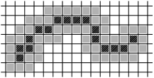
Figure 1: We represent sites as the faces of a square lattice. The striped sites form a path. Together with the grey sites they form the support of a corresponding string operator.
Refer to caption
Figure 2: Geometries involved in the definition of string commutation rules.

Consider the charge group C𝒢C_{\mathcal{G}} of a TSSG. Given a LTI set of generators of 𝒢\mathcal{G}, let us say that the support of ϕ∈Φ⁡(𝒢)\phi\in\Phi(\mathcal{G}) is the set of lattice sites for which there exist a generator gg with support in the site and ϕ⁡(g)=−1\phi(g)=-1. Since the number of charges is finite, we can coarse grain the lattice till each site can hold any of the charges, in the sense that there exists for any site and for any charge c∈C𝒢c\in C_{\mathcal{G}} a morphism ϕ∈Φ0​(𝒢)\phi\in\Phi^{0}(\mathcal{G}) with charge cc and support at that site. Consider two such morphisms ϕ,ϕ′\phi,\phi^{\prime} with the same charge cc but support at different sites σ\sigma, σ′\sigma^{\prime}. Their product has trivial charge so that ϕ​ϕ′=(p,⋅)\phi\phi^{\prime}=(p;\,\cdot\,) for some p∈𝒫p\in\mathcal{P}. Moreover, if we coarse grain enough we can choose pp to have support along a string-shaped region —a thickened path, see Fig. 1— connecting σ\sigma and σ′\sigma^{\prime}. This is a matter of choosing a suitable set of operators pip_{i} for adjacent sites —one per valid ϕ​ϕ′\phi\phi^{\prime} pair—, coarse graining till all the pip_{i} fit in sites adjacent to those involved, and finally forming string operators by composing these pip_{i} operators. We say that pp is a string operator with charge cc and endpoints ϕ\phi, ϕ′\phi^{\prime}. In the case of a TSG 𝒮\mathcal{S} and from the perspective of the Hamiltonian model, a string operator pp of charge cc transports a charge cc from one endpoint to another. E.g., when applied to a ground state pp creates a pair of excitations with charge cc on its endpoints.

Our next goal is to study the commutation properties of strings, which for many geometries only depend on their charges. We start considering three strings p,q,rp,q,r common charge cc and a common endpoint, see Fig. 2(a). The quantity

θ⁡(c):=(p​q;p​r)=(p;q)​(p,r)​(q,r)\theta(c):=(pq;pr)=(p;q)(p;r)(q;r) (11)

only depends on the charge cc, so that it is well defined. To check this, consider an alternative set of strings p′,q′,r′p^{\prime},q^{\prime},r^{\prime} as in Fig. 2(a), together with the auxiliary strings u,v,wu,v,w. Let s=p​q​p′​q′​u​vs=pqp^{\prime}q^{\prime}uv and t=p​r​p′​r′​u​wt=prp^{\prime}r^{\prime}uw. Then (s;t)=(p​q;p​r)​(p′​q′,p′​r′)(s;t)=(pq;pr)(p^{\prime}q^{\prime};p^{\prime}r^{\prime}), but s,t∈𝒵𝒫​(𝒢)∝𝒮s,t\in\mathcal{Z}_{\mathcal{P}}({\mathcal{G}})\propto\mathcal{S} and thus (s,t)=1(s;t)=1 because 𝒮\mathcal{S} is abelian. We can interpret (11) as the topological spin of the charge cc [34]. We say that a charge cc is bosonic if θ⁡(c)=1\theta(c)=1 and fermionic if θ⁡(c)=−1\theta(c)=-1.

Now take two crossing strings p,qp,q with charges c,c′c,c^{\prime}, as in Fig. 2(b). The mutual statistics of the charges cc, dd is given by the quantity [34]

κ⁡(c,d):=(p,q).\kappa(c,d):=(p;q). (12)

It only depends on the charges c,dc,d, so that it is well defined. The proof is analogous to the previous one, now with the geometry of Fig. 2(b). If κ⁡(c,d)=−1\kappa(c,d)=-1 mutual statistics are said to be semionic, otherwise they are trivial. If in Fig. 2(c) pp has charge cc, qq has charge d1d_{1} and rr has charge d2d_{2}, it follows that

κ⁡(c,d1​d2)=κ⁡(c,d1)​κ​(c,d2),\kappa(c,d_{1}d_{2})=\kappa(c,d_{1})\kappa(c,d_{2}), (13)

since κ⁡(c,d1​d2)=(p;q​r)=(p;q)​(p,r)=κ⁡(c,d1)​κ​(c,d2)\kappa(c,d_{1}d_{2})=(p;qr)=(p;q)(p;r)=\kappa(c,d_{1})\kappa(c,d_{2}).

The topological spin and mutual statistics are related. Consider the geometry of Fig. 2(d), where the strings p,q,rp,q,r have charge cc and the strings p′,q′,r′p^{\prime},q^{\prime},r^{\prime} have charge dd. The figure illustrates that

θ⁡(c​d)=θ⁡(c)​θ​(d)​κ​(c,d),\theta(cd)=\theta(c)\theta(d)\kappa(c,d), (14)

since θ⁡(c​d)=(p​p′​q​q′;p​p′​r​r′)=(p​q;p​r)​(p′​q′,p′​r′)​(r,q′)=θ⁡(c)​θ​(d)​κ​(c,d)\theta(cd)=(pp^{\prime}qq^{\prime};pp^{\prime}rr^{\prime})=(pq;pr)(p^{\prime}q^{\prime};p^{\prime}r^{\prime})(r;q^{\prime})=\theta(c)\theta(d)\kappa(c,d). In particular κ⁡(c,c)=1.\kappa(c,c)=1.

In summary, the charges in C𝒢C_{\mathcal{G}} can be regarded as the topological charges of an anyon model, with fusion given by the charge group product. But the topological structure does not stop there, because it is possible to define κ\kappa for a string with charge in C𝒮C_{\mathcal{S}} and another with charge in C𝒢C_{\mathcal{G}}. This works because 𝒵𝒫​(𝒮)⊂𝒵𝒫​(𝒵𝒫​(𝒢))\mathcal{Z}_{\mathcal{P}}({\mathcal{S}})\subset\mathcal{Z}_{\mathcal{P}}({\mathcal{Z}_{\mathcal{P}}({\mathcal{G}})}), which is all we need for the construction in Fig. 2(b) to make sense. We cannot define κ\kappa for two strings with charges in C𝒮C_{\mathcal{S}}, nor can we define θ\theta for charges in C𝒮C_{\mathcal{S}}, unless of course we are dealing with a TSG rather than a general T​S​S​GTSSG. Therefore, we should regard the charges in C𝒢C_{\mathcal{G}} as anyons, and the charges in C𝒮C_{\mathcal{S}} as fluxes that interact topogically with these anyons through an Aharonov-Bohm effect.

There is a natural morphism Cι:C𝒢⟶C𝒮C_{\iota}:\,C_{\mathcal{G}}\longrightarrow C_{\mathcal{S}} derived from the restriction of morphisms from 𝒢\mathcal{G} to morphisms from 𝒮\mathcal{S}. It preserves commutation in the sense that κ⁡(c,d)=κ⁡(Cι​(c),d)\kappa(c,d)=\kappa(C_{\iota}(c),d) for c,d∈C𝒢c,d\in C_{\mathcal{G}}. This is an important ingredient in the construction of canonical charge generators given in theorem 36:

C𝒢=⟨c1,…,cα,d1,…,dα,e1,…,eβ⟩,c~i=Cι​(di),\displaystyle C_{\mathcal{G}}=\langle c_{1},\dots,c_{\alpha},d_{1},\dots,d_{\alpha},e_{1},\dots,e_{\beta}\rangle,\qquad\quad\tilde{c}_{i}=C_{\iota}(d_{i}),
C𝒮=⟨c~1,…,c~α,d~1,…,d~α,e~1,…,e~β⟩,d~i=Cι​(ci),\displaystyle C_{\mathcal{S}}=\langle\tilde{c}_{1},\dots,\tilde{c}_{\alpha},\tilde{d}_{1},\dots,\tilde{d}_{\alpha},\tilde{e}_{1},\dots,\tilde{e}_{\beta}\rangle,\qquad\quad\tilde{d}_{i}=C_{\iota}(c_{i}), (15)

where i=1,…,αi=1,\dots,\alpha, the eie_{i} generate the kernel of CιC_{\iota} and all gauge charge generators are bosons except possibly e1e_{1}, c1c_{1} and d1d_{1}, always with θ⁡(c1)=θ⁡(d1)\theta(c_{1})=\theta(d_{1}). Among gauge charge generators the only nontrivial mutual statistcs are κ⁡(ci,di)=−1\kappa(c_{i},d_{i})=-1. The mutual statistics between gauge and stabilizer charges gives rise to the duality. Indeed, relabeling C𝒢=⟨c1,…,c2​α+β⟩C_{\mathcal{G}}=\langle c_{1},\dots,c_{2\alpha+\beta}\rangle, C𝒮=⟨c~1,…,c~2​α+β⟩C_{\mathcal{S}}=\langle\tilde{c}_{1},\dots,\tilde{c}_{2\alpha+\beta}\rangle,

κ⁡(ci,c~j)=1−2​δi​j,i,j=1,…,2​α+β.\kappa(c_{i},\tilde{c}_{j})=1-2\delta_{ij},\qquad i,j=1,\dots,2\alpha+\beta. (16)

The anyon model attached to C𝒢C_{\mathcal{G}} only has a few parameters, α\alpha, β\beta, χ=θ⁡(c1)\chi=\theta(c_{1}) and f=θ⁡(e1)f=\theta(e_{1}). We call this the characteristic of the TSSG. The anyon model is chiral when χ=−1\chi=-1, and when f=−1f=-1 there are fermions among the eie_{i}. There exist TSSGs covering all possible combinations of these parameters, as shown in section 7.2. Since the subsystem toric code only has a nontrivial element in C𝒢C_{\mathcal{G}} it is an example of a TSSG with α=0\alpha=0 and β=1\beta=1. Moreover, string operators are products of single qubit ZZ Pauli operators, and thus f=1f=1.

In the case of TSGs β=0\beta=0, leaving the parameters α\alpha and χ\chi. The toric code has α=1\alpha=1 and χ=1\chi=1, and thus combining NN toric codes together we get a code with α=N\alpha=N and χ=1\chi=1. Chiral codes are not likely to exist [7].

2.7 Code structure and homology
Refer to caption
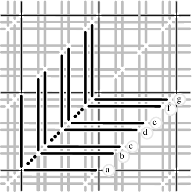
Figure 3: Framework of string segments. Each charge contributes a square lattice.

With string operators and their geometrical commutation relations at hand, it is easy to uncover the general structure of TSSGs. Given a TSSG, we can put it in a standard form —its prototype is the toric code— through the following process. The first step is to find a set of canonical charges. Then we construct a translationally invariant framework of string operators, each in the form of a straight segment. For each charge there is a square lattice of segment operators, spatially disposed as indicated in Fig. 3. With suitable adjustments, the commutation relations between these segments operators are fixed by θ\theta and κ\kappa. Strings with charge cic_{i} (did_{i}) also have charge d~i\tilde{d}_{i} (c~i\tilde{c}_{i}), and we adjust segment operators with charge eie_{i} so that they are elements of 𝒢\mathcal{G} —in the technical part we impose more structure on those with charge e~i\tilde{e}_{i}, but it does not affect the present discussion, only that of local equivalence.

Refer to caption
Figure 4: (Left) A square lattice and its dual. String operators can be visualized as collections of segments on these two lattices. We show for such strings: a direct plaquette, a dual plaquette, a direct boundary and a dual open string. The last two cross once. (Right) Logical operators corresponding to strings with charge cic_{i}, in black, and strings with charge did_{i}, in grey, for any i=1,…,αi=1,\dots,\alpha. The topology is that of a torus, with opposite boundaries identified.

Rather than the intricate framework of Fig. 3, it is enough to visualize, for each pair of dual charges ci,dic_{i},d_{i} (or ei,e~ie_{i},\tilde{e}_{i}) a single square lattice and its dual, see Fig. 4. Segment operators with charge cic_{i} or eie_{i} belong to the direct lattice, and those with charge did_{i} or e~i\tilde{e}_{i} to the dual lattice. We can form string operators by taking products of segment operators with the same charge. Operators from different lattices commute, and the commutation properties of string operators are simply dictated by κ\kappa and θ\theta. E.g., a direct string with charge cic_{i} anticommutes with a dual string of charge did_{i} iff the two strings cross an odd number of times.

Closed strings operators —or boundary strings since the homology is trivial in the plane— belong to 𝒮\mathcal{S} or at least to 𝒢\mathcal{G} —the former is the case of e~i\tilde{e}_{i} closed strings. Any boundary operator is a product of ‘plaquette operators’, each of them the product of the segment operators forming a plaquette. Crucially, it is possible to find LTI sets of independent generators of 𝒢\mathcal{G} and 𝒮\mathcal{S} that include these plaquette operators, which are the only ones subject to constraints —now obvious. In particular, those plaquette operators formed by c~i,d~i\tilde{c}_{i},\tilde{d}_{i} or e~i\tilde{e}_{i} (cic_{i}, did_{i} or eie_{i}) strings are generators of 𝒮\mathcal{S} (𝒢\mathcal{G}).

The trivial stabilizer generators, i.e., those that are not plaquette operators, play no significant role, in the sense that it is always possible to find a local transformation that removes them as disentangled qubits. After this removal, we are left with a system where every Pauli operator can be decomposed as s​gsg, where ss is a product of string operators and gg is a product of trivial gauge generators.

2.8 Back to codes

The homological perspective on string operators becomes most relevant when we go back to a code in a finite lattice, as we sketch here. The simplest possible way to do this is by considering a finite lattice with periodic boundary conditions, so that the topology is that of a torus. The decomposition in terms of string operators and trivial gauge generators still holds —the lattice must be large enough, though, in terms of the support of the segment operators and trivial gauge generators. But now closed string operators need not be boundaries, and this is an all-important feature.

Regarding gauge and stabilizer generators, each ‘global constraint’ becomes now a constraint of the form ∏ipi∝1\prod_{i}p_{i}\propto 1, with pip_{i} running over plaquette operators of a given lattice, direct or dual, so that we can remove one such plaquette from the corresponding generating sets. But this still does not give rise in general to a proper stabilizer and gauge group pair. Indeed, when β≠0\beta\neq 0 we have to either add nontrivial cycle strings with charge eie_{i} to 𝒮\mathcal{S} or nontrivial cycle string with charge e~i\tilde{e}_{i} to 𝒢\mathcal{G}. This does not affect the number of encoded qubits —but see below!. In fact, apart from this detail everything works as in a toric code. Each pair (ci,di)(c_{i},d_{i}) contributes two logical qubits, so that k=2​αk=2\alpha, and logical operators correspond to nontrivial cycles, see Fig. 4.

From the above discussion it seems that the existence of the β\beta charges eje_{j} serves no purpose from a coding perspective. For quantum codes this is indeed true in the sense that they contribute no encoded qubits. However, interestingly they do provide encoded bits! The eigenvalues of nontrivial closed strings with charge e~i\tilde{e}_{i} label the classical states of the memory —and should be regarded as elements of 𝒢\mathcal{G}—, and nontrivial closed string operators with charge eie_{i} act as bit flip operators. Detecting errors thus amount to look for the endpoint of open string operators with charge eie_{i}. I.e., the stabilizer —which must include only strings of trivial homology—, still provides the error syndrome through the eigenvalues of its generators. The subsystem toric code exemplifies all this.

2.9 Equivalence

We say that two TSSGs are locally equivalent if they can be related by a combination of LTI Clifford transformations, lattice coarse graining and addition/removal of disentangled qubits in a translationally invariant way. Such local transformations preserve the topological charge structure, and the converse also holds in some cases, see section 8.4:

Non-chiral TSSGs are locally equivalent iff they have the same characteristic.

This result, true also for chiral TSGs, is a consequence of the structure discussed above, together with the existence of certain ‘elementary’ TSSGs and the ability to ‘complete’ partially defined LTI Clifford transformations, see lemma 2.

2.10 Centralizers and 2D topology

Refer to caption
Figure 5: The regions involved in the construction of an LTI set of independent generators.

To finish this summary of results, let us explain the role played by the topology of the plane and the fact that the LPG is a centralizer of a LPG for the existence of an LTI set of independent generators. Let the support of a constraint be the union of the support of its elements. Consider a LPG 𝒜\mathcal{A} of the form 𝒜=𝒵𝒫​(ℬ)\mathcal{A}=\mathcal{Z}_{\mathcal{P}}({\mathcal{B}}). In order to recover a LTI set of independent generators from an arbitrary LTI set of generators of 𝒜\mathcal{A}, all we need to do is remove in a translationally invariant way a sufficient amout of generators. If a generator is part of a constraint, it can be removed. The removal of constrained generators with support in the regions AA, marked with dark grey in Fig. 5(a), can be done without much difficulty. It is enough to choose a large enough separation between these regions, so that generators in different regions are subject to independent constraints, which allows a translationally invariant removal. After the removal it is unclear whether the generators with support in different regions BB, marked with light grey in Fig. 5(a), are also subject to independent constraints. But given a constraint RR with support, say, in the region B0B_{0} marked with stripes in Fig. 5(a), we can find —as shown below— another constraint R0R_{0} containing the same generators as RR in B0B_{0} but with no support in the rest of regions BB. This shows that generators with support in different regions BB are indeed subject to independent constraints. Then we are left with the regions CC, marked with white in Fig. 5(a), but these are disconnected from each other and we can deal with them as follows. The constraints that are left can only include generators with support in regions CC now, and since they are distant enough and the generators are local, the restriction of any constraint to a particular region CC is still a constraint. Thus, generators with support in different regions CC are also subject to independent constraints.

Thus, the crucial point is the existence, for any given constraint RR with support in regions BB and CC, of a constraint R0R_{0} with the same support as RR in B0B_{0} but no support in other regions BB. To guarantee it, we take the size of the regions AA as large as needed, so that near B0B_{0} any such RR has support only in a long and narrow band. Then, up to translations, the elements in RR must repeat along the band at certain stretches of a length larger than the size of the generators. At each side of the band we pick two such repeated stretches, marked with stripes in Fig. 5(b), and form a new constraint R∞R_{\infty} that extendes to infinity by repeating the set of constraints in between the repeated stretches up to translations. This is depicted in Fig. 5(c), where the places where the repeated stretches overlap are marked with stripes and the support of R∞R_{\infty} is darkened. We can then consider a subset of R∞R_{\infty}, containing only the elements on the darkened region in Fig. 5(d), which produces a set of generators SS with product p1​p2∈𝒫p_{1}p_{2}\in\mathcal{P}, where pip_{i} have each support in one of the two regions marked with stripes. The all-important property of these two regions is that they are sufficiently far away from region AA. Since p1​p2∈𝒵𝒫​(ℬ)p_{1}p_{2}\in\mathcal{Z}_{\mathcal{P}}({\mathcal{B}}) and ℬ\mathcal{B} has local generators, it follows that p1,p2∈𝒵𝒫​(ℬ)p_{1},p_{2}\in\mathcal{Z}_{\mathcal{P}}({\mathcal{B}}) since the supports of p1p_{1} and p2p_{2} are sufficiently far appart. There exist sets of generators SiS_{i} of 𝒜\mathcal{A}, i=1,2i=1,2, with supports in a small neighborhood of the support of pip_{i} and such that their product is proportional to pip_{i}. Then to obtain R0R_{0} it is enough to take the symmetric difference of SS, S1S_{1} and S2S_{2}.

3 Basic definitions

This section intends to put together most of the constructions needed later, with the aim of both presenting them and serving as a reference for later sections. It includes a list of basic examples of topological codes.

3.1 Notation

Sets — For integers we use the notation 𝐍0:={0}∪𝐍∗\mathbf{N}_{0}:=\{0\}\cup\mathbf{N}^{\ast}. |S||S| denotes the cardinality of a set SS, 𝐏⁡(S){\bf P}(S) its power set and 𝐏0​(S):={s∈𝐏⁡(S):|s|<ℵ0}.{\bf P}_{0}(S):=\{s\in{\bf P}(S)\,:\,|s|<\aleph_{0}\}. Given a mapping f:A⟶Bf:\,A\longrightarrow B and any subsets a⊂Aa\subset A, b⊂Bb\subset B, we denote by f⁡[a]⊂Bf[a]\subset B the image of aa and by f−1​[b]⊂Af^{-1}[b]\subset A the preimage of bb. Given any set SS, we regard 𝐏⁡(S){\bf P}(S) as the abelian group with addition given by the symmetric difference S1+S2:=S1∪S2−S1∩S2.S_{1}+S_{2}:=S_{1}\cup S_{2}-S_{1}\cap S_{2}.

2D lattice — Since we are interested in topological aspects, we consider without loss of generality square lattices. Sites are labeled as usual with integer coordinates (j,k)∈𝐙2(j,k)\in\mathbf{Z}^{2}, with Σ=𝐙2\Sigma=\mathbf{Z}^{2} the set of all sites, and 𝟎:=(0,0){\mathbf{0}}:=(0,0). A block is a set of sites of the form

□m,nm′,n′:={(j,k):m≤j<m′;n≤k<n′}.\square_{m,n}^{m^{\prime},n^{\prime}}:=\{(j,k)\,:\,m\leq j<m^{\prime};n\leq k<n^{\prime}\}. (17)

Given a set of sites γ∈𝐏0​(Σ)\gamma\in{\bf P}_{0}(\Sigma), ρ⁡(γ)\rho(\gamma) denotes the smallest k∈𝐍0k\in\mathbf{N}_{0} such that γ⊂□m,nm+k,n+k\gamma\subset\square_{m,n}^{m+k,n+k} for some m,n∈𝐙m,n\in\mathbf{Z}. For γ⊂Σ\gamma\subset\Sigma, l∈𝐍0l\in\mathbf{N}_{0}, define a ‘thickened’ set

Thkl​(γ):=⋃(i,j)∈γ□i−l,j−li+l+1,j+l+1.\mathrm{Thk}^{l}(\gamma):=\bigcup_{(i,j)\in\gamma}\square_{i-l,j-l}^{i+l+1,j+l+1}. (18)

Connectedness — Two sites (i,j)(i,j) and (m,n)(m,n) are adjacent if |m−i|≤1|m-i|\leq 1 and |n−j|≤1|n-j|\leq 1. An ordered list of sites (σk)k=1n=(σ0,⋯,σn)(\sigma_{k})_{k=1}^{n}=(\sigma_{0},\cdots,\sigma_{n}) where σk\sigma_{k} is adjacent to σk+1\sigma_{k+1} for all k=1,…,nk=1,\dots,n is a path from σ0\sigma_{0} to σn\sigma_{n}. We define the inverse γ−1\gamma^{-1} of a path γ\gamma in the usual way, an also the composition of paths γ′∘γ\gamma^{\prime}\circ\gamma, where the last site of γ\gamma is the first site of γ′\gamma^{\prime}. A set of sites γ⊂Σ\gamma\subset\Sigma is connected if for any σ,σ′∈γ\sigma,\sigma^{\prime}\in\gamma there exists a path (σk)k=1n(\sigma_{k})_{k=1}^{n} with σ0=σ\sigma_{0}=\sigma, σn=σ′\sigma_{n}=\sigma^{\prime} and σi∈γ\sigma_{i}\in\gamma, i=1,…,ni=1,\dots,n. Given an ordered set of sites (σk)k=1n=((ak,bk))k=1n(\sigma_{k})_{k=1}^{n}=((a_{k},b_{k}))_{k=1}^{n}, let σk′:=(ak+1,bk),\sigma_{k}^{\prime}:=(a_{k+1},b_{k}), k=1,…,n−1k=1,\dots,n-1 and define Path⁡(σ1,…,σn)\mathrm{Path}(\sigma_{1},\dots,\sigma_{n}) to be the path starting at σ1\sigma_{1}, moving in a straight line to σ1′\sigma_{1}^{\prime}, then in a straight line to σ2\sigma_{2}, then σ2′\sigma_{2}^{\prime},…, and ending at σn\sigma_{n}. Sometimes we identify a path (σi)(\sigma_{i}) with the set {σi}\{\sigma_{i}\}.

Homology — Let Γ\Gamma be an infinite square lattice. Γfc{\Gamma_{\mathrm{fc}}}, Γfc∗{\Gamma_{\mathrm{fc}}^{\ast}}, Γedg{\Gamma_{\mathrm{edg}}} and Γedg∗{\Gamma_{\mathrm{edg}}^{\ast}} denote, respectively, the set of faces, dual faces, edges and dual edges. We represent 𝐙2\mathbf{Z}_{2} chains of these objects as elements of 𝐏⁡(Γfc){\bf P}({\Gamma_{\mathrm{fc}}}), 𝐏⁡(Γfc∗){\bf P}({\Gamma_{\mathrm{fc}}^{\ast}}), 𝐏⁡(Γedg){\bf P}({\Gamma_{\mathrm{edg}}}) and 𝐏⁡(Γedg∗){\bf P}({\Gamma_{\mathrm{edg}}^{\ast}}). ∂\partial denotes the usual boundary operation, which we express in particular as

𝐏⁡(Γfc)​⟶∂​𝐏​(Γedg)​⟶∂​𝐏​(Γfc∗),𝐏⁡(Γfc∗)​⟶∂​𝐏​(Γedg∗)​⟶∂​𝐏​(Γfc).\displaystyle{\bf P}({\Gamma_{\mathrm{fc}}})\,\overset{\partial}{\longrightarrow}\,{\bf P}({\Gamma_{\mathrm{edg}}})\,\overset{\partial}{\longrightarrow}\,{\bf P}({\Gamma_{\mathrm{fc}}^{\ast}}),\qquad{\bf P}({\Gamma_{\mathrm{fc}}^{\ast}})\,\overset{\partial}{\longrightarrow}\,{\bf P}({\Gamma_{\mathrm{edg}}^{\ast}})\,\overset{\partial}{\longrightarrow}\,{\bf P}({\Gamma_{\mathrm{fc}}}). (19)

Given an edge ee, it dual is denoted e∗e^{\ast}. We name the elements 𝐞1,𝐞2∈Γedg\boldsymbol{\mathrm{e}}_{1},\boldsymbol{\mathrm{e}}_{2}\in{\Gamma_{\mathrm{edg}}}, 𝐟∈Γfc,𝐟∗∈Γfc∗\boldsymbol{\mathrm{f}}\in{\Gamma_{\mathrm{fc}}},\boldsymbol{\mathrm{f}}^{\ast}\in{\Gamma_{\mathrm{fc}}^{\ast}} according to Fig. 6. For faces, the symbol ∗ is just a label.

Refer to caption
Figure 6: Naming some elements of Γ\Gamma.

Qubits and operators — Sites hold a common and finite number of qubits nn. Let Xj,kαX_{j,k}^{\alpha}, Zj,kαZ_{j,k}^{\alpha} denote single qubit XX and ZZ operators acting on the qubit with label α=1,…,n\alpha=1,\dots,n on the site (j,k)(j,k). They generate for each site (j,k)(j,k) an algebra of operators A(j,k)A_{(j,k)}. Consider the infinite tensor product A:=⊗(j,k)A(j,k)A:=\otimes_{(j,k)}A_{(j,k)}, with elements ⊗(j,k)a(j,k)\otimes_{(j,k)}a_{(j,k)} with all but a finite number of the product terms identical a(j,k)=𝟏a_{(j,k)}=\mathbf{1}. The Pauli group 𝒫⊂A\mathcal{P}\subset A is 𝒫:=⟨i​𝟏⟩​⟨Xi​jα,Zi​jα⟩i,j,α.\mathcal{P}:=\langle i\mathbf{1}\rangle\langle X_{ij}^{\alpha},Z_{ij}^{\alpha}\rangle_{i,j,\alpha}. Given a Pauli operator p∈𝒫p\in\mathcal{P}, Supp⁡(p)\mathrm{Supp}(p) denotes the set of sites containing qubits on the support of pp, i.e., on which pp acts nontrivially. Its size is measured by ρ⁡(p):=ρ⁡(Supp⁡(p))\rho(p):=\rho(\mathrm{Supp}(p)). For γ⊂Σ\gamma\subset\Sigma we let p|γp|_{\gamma} be the restriction of pp to qubits in γ\gamma, defined in the obvious way and only up to a global phase. Given p,q∈𝒫p,q\in\mathcal{P} their commutator is (p;q):=p​q​p−1​q−1=±1.(p;q):=pqp^{-1}q^{-1}=\pm 1. For 𝒜,ℬ⊂𝒫\mathcal{A},\mathcal{B}\subset\mathcal{P}, the centralizer of 𝒜\mathcal{A} in ℬ\mathcal{B} is

𝒵ℬ(𝒜):={b∈ℬ:∀a∈𝒜(a;b)=1}.\mathcal{Z}_{\mathcal{B}}({\mathcal{A}}):=\{b\in\mathcal{B}\,:\,\forall a\in\mathcal{A}\quad(a;b)=1\}. (20)

We write 𝒜∝ℬ\mathcal{A}\propto\mathcal{B} meaning ⟨i​𝟏⟩​𝒜=⟨i​𝟏⟩​ℬ\langle i\mathbf{1}\rangle\mathcal{A}=\langle i\mathbf{1}\rangle\mathcal{B}.

Pauli group subsets — For S⊂𝒫S\subset\mathcal{P}, γ⊂Σ\gamma\subset\Sigma and q∈𝒫q\in\mathcal{P} we define

Supp⁡(S):=⋃Supp⁡[S],\displaystyle\mathrm{Supp}(S):=\bigcup\mathrm{Supp}[S],\qquad S|γ:={s∈S:Supp⁡(s)⊂γ},\displaystyle S|_{\gamma}:=\{s\in S\,:\,\mathrm{Supp}(s)\subset\gamma\},
S||γ:={s∈S:Supp(s)∩γ≠∅},\displaystyle S||_{\gamma}:=\{s\in S\,:\,\mathrm{Supp}(s)\cap\gamma\neq\emptyset\},\qquad (S;q):=∏p∈Sq(p;q),\displaystyle(S;q):=\prod_{p\in S_{q}}(p;q), (21)

where Sq={p∈S:Supp⁡(p)∩Supp⁡(q)≠∅}S_{q}=\{p\in S\,:\,\mathrm{Supp}(p)\cap\mathrm{Supp}(q)\neq\emptyset\} and only for SqS_{q} finite the definition holds. We set ρ⁡(S):=ρ⁡(Supp⁡(S)).\rho(S):=\rho(\mathrm{Supp}(S)). We say that a set of generators 𝒜g\mathcal{A}_{g} of a group 𝒜⊂𝒫\mathcal{A}\subset\mathcal{P} is independent if the product of any finite subset of nontrivial generators is nontrivial —trivial elements of 𝒫\mathcal{P} are those in ⟨i​𝟏⟩\langle i\mathbf{1}\rangle. We define a ‘product’ group morphism

Pro:𝐏0​(𝒫)\displaystyle\mathrm{Pro}\,:\,\,{\bf P}_{0}(\mathcal{P}) ⟶𝒫/⟨i​𝟏⟩\displaystyle\longrightarrow\mathcal{P}/\langle i\mathbf{1}\rangle
S\displaystyle S ⟼⟨i​𝟏⟩​∏p∈Sp.\displaystyle\longmapsto\langle i\mathbf{1}\rangle\prod_{p\in S}p. (22)

Morphisms — Let 𝒜⊂𝒫\mathcal{A}\subset\mathcal{P} be a group. The group morphisms ϕ:𝒜⟶{1,−1}\phi:\,\mathcal{A}\longrightarrow\{1,-1\} such that ϕ⁡(i)=1\phi(i)=1 form an abelian group Φ⁡(𝒜)\Phi(\mathcal{A}) with (ϕ​ϕ′)​(a):=ϕ⁡(a)​ϕ′​(a).(\phi\phi^{\prime})(a):=\phi(a)\phi^{\prime}(a). Given a subset 𝒜g\mathcal{A}_{g} of 𝒜\mathcal{A}, we define a group morphism

Neg𝒜g:Φ⁡(𝒜)\displaystyle\mathrm{Neg}_{\mathcal{A}_{g}}\,:\,\,\Phi(\mathcal{A}) ⟶𝐏⁡(𝒜g−⟨i​𝟏⟩)\displaystyle\longrightarrow{\bf P}(\mathcal{A}_{g}-\langle i\mathbf{1}\rangle)
ϕ\displaystyle\phi ⟼𝒜g∩ϕ−1​[−1],\displaystyle\longmapsto\mathcal{A}_{g}\cap\phi^{-1}[-1], (23)

which has an inverse Neg𝒜g−1\mathrm{Neg}_{\mathcal{A}_{g}}^{-1} if 𝒜g\mathcal{A}_{g} is an independent set of generators of 𝒜\mathcal{A}. The support of ϕ∈Φ⁡(𝒜)\phi\in\Phi(\mathcal{A}) with respect to 𝒜g\mathcal{A}_{g} is

Supp𝒜g​(ϕ):=Supp⁡(Neg𝒜g​(ϕ)).\mathrm{Supp}_{\mathcal{A}_{g}}(\phi):=\mathrm{Supp}(\mathrm{Neg}_{\mathcal{A}_{g}}(\phi)). (24)

We define the subgroup of morphisms with finite support

Φ0​(𝒜g):={ϕ∈Φ⁡(⟨𝒜g⟩):|Supp𝒜g​(ϕ)|<ℵ0}.\Phi^{0}(\mathcal{A}_{g}):=\{\phi\in\Phi(\langle\mathcal{A}_{g}\rangle)\,:\,|\mathrm{Supp}_{\mathcal{A}_{g}}(\phi)|<\aleph_{0}\}. (25)

Given ϕ∈Φ0​(𝒜g)\phi\in\Phi^{0}(\mathcal{A}_{g}), we will denote with the same name the group morphism

ϕ:𝐏⁡(𝒜g)\displaystyle\phi\,:\,\,{\bf P}(\mathcal{A}_{g}) ⟶{1,−1}\displaystyle\longrightarrow\{1,-1\}
S\displaystyle S ⟼(−1)|S∩Neg𝒜g​(ϕ)|\displaystyle\longmapsto(-1)^{|S\cap\mathrm{Neg}_{\mathcal{A}_{g}}(\phi)|} (26)

The commutation structure gives rise to morphisms that need a name,

Com𝒜:𝒫\displaystyle\mathrm{Com}_{\mathcal{A}}\,:\,\mathcal{P} ⟶Φ⁡(𝒜)\displaystyle\longrightarrow\Phi(\mathcal{A})\qquad Com𝒜:𝐏⁡(𝒫)\displaystyle\mathrm{Com}_{\mathcal{A}}\,:\,{\bf P}(\mathcal{P}) ⟶Φ⁡(𝒜)\displaystyle\longrightarrow\Phi(\mathcal{A})
p\displaystyle p ⟼(p,⋅)\displaystyle\longmapsto(p;\cdot)\qquad S\displaystyle S ⟼(S,⋅)\displaystyle\longmapsto(S;\cdot) (27)

For p∈𝒫p\in\mathcal{P} or p∈𝐏⁡(𝒫)p\in{\bf P}(\mathcal{P}) we set Supp𝒜g​(p):=Supp𝒜g​((,,,)).\mathrm{Supp}_{\mathcal{A}_{g}}(p):=\mathrm{Supp}_{\mathcal{A}_{g}}((p;\cdot)).

Translation operators — We define translation operators for sites setting

Tm,n​(j,k):=(j+m,k+n).T_{m,n}\,(j,k):=(j+m,k+n). (28)

The action on edges or faces of Γ\Gamma is analogous. For Pauli operators we define Tm,n:𝒫⟶𝒫T_{m,n}\,:\,\mathcal{P}\longrightarrow\mathcal{P} as group morphisms with Tm,n​(i​𝟏):=i​𝟏T_{m,n}\,(i\mathbf{1}):=i\mathbf{1} and

Tm,n(σj,kα):=σj+m,k+nα,σ=X,Z.T_{m,n}\,(\sigma_{j,k}^{\alpha}):=\sigma_{j+m,k+n}^{\alpha},\qquad\sigma=X,Z. (29)

For ϕ∈Φ⁡(𝒜)\phi\in\Phi(\mathcal{A}) we set

(Tm,n​(ϕ))​(⋅):=ϕ⁡(T−m,−n​(⋅)).(T_{m,n}\,(\phi))(\cdot):=\phi(T_{-m,-n}\,(\cdot)). (30)

To generalize translation to sets of translatable objects, we recursively define whenever it makes sense

Tm,n​(A):={Tm,n​(a):a∈A}.T_{m,n}\,(A):=\{T_{m,n}\,(a)\,:\,a\in A\}. (31)

Finally, we set for d∈𝐍∗d\in\mathbf{N}^{\ast}

T(d)​(⋅):=⋃m,n∈𝐙Tm​d,n​d​(⋅).T^{(d)}\,(\cdot):=\bigcup_{m,n\in\mathbf{Z}}T_{md,nd}\,(\cdot). (32)

Coarse graining and composition — A qubit lattice can be coarse grained by identifying each block □m​l,n​l(m+1)​l,(n+1)​l\square_{ml,nl}^{(m+1)l,(n+1)l} as the site (m,n)(m,n) of the new lattice, for some l∈𝐍∗l\in\mathbf{N}^{\ast}. We denote the effect of coarse graining on a given object xx by Crsl​(x)\mathrm{Crs}_{\hskip 0.3ptl}(x), be it an operator, a set of sites, a group or any other structure.

Two disjoint qubit lattices can be put together to form a single lattice. If 𝒜\mathcal{A} is a Pauli subgroup on the first lattice and ℬ\mathcal{B} is a Pauli subgroup on the second lattice we define a new group 𝒜⊗ℬ:={a⊗b:a∈𝒜,b∈ℬ}.\mathcal{A}\otimes\mathcal{B}:=\{a\otimes b\,:\,a\in\mathcal{A},b\in\mathcal{B}\}.

3.2 Lattice Pauli morphism

Consider Pauli groups 𝒫i\mathcal{P}_{i} over square lattices.

Definition 1

A lattice Pauli (iso)morphism is a group (iso)morphism F:𝒫1⟶𝒫2F:\,\mathcal{P}_{1}\longrightarrow\mathcal{P}_{2} such that F⁡(i)=iF(i)=i and, for any m,n∈𝐙m,n\in\mathbf{Z} and some d∈𝐍∗d\in\mathbf{N}^{\ast},

Tm​d,n​d∘F=F∘Tm​d,n​d.T_{md,nd}\,\circ F=F\circ T_{md,nd}\,. (33)

We say that FF has period dd and define

ρ⁡(F):=maxσ∈□0,0d,d⁡ρ⁡({σ}∪Supp⁡(F⁡[𝒫1|{σ}])).\rho(F):=\max_{\sigma\in\square_{0,0}^{d,d}}\rho(\{\sigma\}\cup\mathrm{Supp}(F[\mathcal{P}_{1}|_{\{\sigma\}}])). (34)

Such a morphism is always injective. ρ⁡(F)\rho(F) is finite and

Supp⁡(F⁡(p))⊂Thkρ⁡(F)−1​(Supp⁡(p))\mathrm{Supp}(F(p))\subset\mathrm{Thk}^{\rho(F)-1}(\mathrm{Supp}(p)) (35)

for every p∈𝒫1p\in\mathcal{P}_{1}. By coarse graining we can always have d=1d=1 and ρ⁡(F)=2\rho(F)=2. If nin_{i} is the number of qubits per site in 𝒫i\mathcal{P}_{i}, n1≤n2n_{1}\leq n_{2} and the equality holds iff FF is an isomorphism. To see way, take γ=□0,0L,L\gamma=\square_{0,0}^{L,L} and let g1=2​n1​L2g_{1}=2n_{1}L^{2} be the number of generators of 𝒫1′:=𝒫1|γ\mathcal{P}_{1}^{\prime}:=\mathcal{P}_{1}|_{\gamma} and g2=2​n2​(L+2​ρ​(F)−2)2g_{2}=2n_{2}(L+2\rho(F)-2)^{2} be the number of generators of 𝒫2′:=𝒫2|Thkρ⁡(F)−1​(γ)\mathcal{P}_{2}^{\prime}:=\mathcal{P}_{2}|_{\mathrm{Thk}^{\rho(F)-1}(\gamma)}. Then F⁡[𝒫1′]⊂𝒫2′F[\mathcal{P}_{1}^{\prime}]\subset\mathcal{P}_{2}^{\prime} gives g1≤g2g_{1}\leq g_{2} and thus in the limit of large LL we get the desired result. The following ‘extension lemma’ will be very useful later and is true for any spatial dimensionality.

Lemma 2

For every lattice Pauli morphism F:𝒫1⟶𝒫3F:\,\mathcal{P}_{1}\longrightarrow\mathcal{P}_{3} there exist 𝒫2\mathcal{P}_{2} and a lattice Pauli isomorphism Fe​x​t:𝒫1⊗𝒫2⟶𝒫3F_{\mathrm{e}xt}:\,\mathcal{P}_{1}\otimes\mathcal{P}_{2}\longrightarrow\mathcal{P}_{3} with the same period and

Fe​x​t​(p⊗𝟏)=F⁡(p).F_{\mathrm{e}xt}(p\otimes\mathbf{1})=F(p). (36)

Since Fe​x​tF_{\mathrm{e}xt} preserve centralizers, there exists G:𝒫2⟶𝒫3G:\,\mathcal{P}_{2}\longrightarrow\mathcal{P}_{3} with

Fext​(p⊗q)=F⁡(p)​G​(q),G⁡[𝒫2]=𝒵𝒫3​(F⁡[𝒫1]).F_{\mathrm{ext}}(p\otimes q)=F(p)G(q),\quad G[\mathcal{P}_{2}]=\mathcal{Z}_{\mathcal{P}_{3}}({F[\mathcal{P}_{1}]}). (37)

Proof — In this proof we need to deal with ‘regions’ that are collections of qubits, rather than of complete sites. So let Σ⁡(α)\Sigma(\alpha) denote all qubits with label α\alpha and 𝒫iα:=𝒫i|Σ⁡(α)\mathcal{P}_{i}^{\alpha}:=\mathcal{P}_{i}|_{\Sigma(\alpha)}. We can assume w.l.o.g. d=1d=1. To avoid trivial cases we assume 1≤n1<n31\leq n_{1}<n_{3}, and set n2=n3−n1n_{2}=n_{3}-n_{1}. If we can construct a lattice Pauli isomorphism F′:𝒫3⟶𝒫1⊗𝒫2F^{\prime}:\,\mathcal{P}_{3}\longrightarrow\mathcal{P}_{1}\otimes\mathcal{P}_{2} with period 1 and such that F′​(F⁡(⋅))=F′′​(⋅)⊗𝟏F^{\prime}(F(\cdot))=F^{\prime\prime}(\cdot)\otimes\mathbf{1} for some isomorphism F′′:𝒫1⟶𝒫1F^{\prime\prime}:\,\mathcal{P}_{1}\longrightarrow\mathcal{P}_{1}, the result follows taking Fe​x​t=F′−1∘(F′′⊗𝐈𝒫2)F_{\mathrm{e}xt}={F^{\prime}}^{-1}\circ(F^{\prime\prime}\otimes{\bf I}_{\mathcal{P}_{2}}). We construct F′F^{\prime} as a composite F′=Fb∘FaF^{\prime}=F_{b}\circ F_{a}. In turn, Fa:𝒫3⟶𝒫3F_{a}:\,\mathcal{P}_{3}\longrightarrow\mathcal{P}_{3} is composed of two kinds of maps. The first kind is that of single qubit Clifford gates, preserving translational invariance. The second corresponds to CNot gates applied to pairs of qubits with different label α\alpha —but possibly in different sites— again preserving translational invariance. Composing such ‘moves’, it is a routine computation —we are essentially back to a finite Pauli group case, with the restriction of not being able to perform CNot gates between qubits with the same label— to construct an isomorphism F1F_{1} such that F1′​[𝒫11|𝟎]⊂𝒫31F_{1}^{\prime}[\mathcal{P}_{1}^{1}|_{{\mathbf{0}}}]\subset\mathcal{P}_{3}^{1} for F1′:=F1∘FF_{1}^{\prime}:=F_{1}\circ F. Then we have F1′​[𝒫11]=𝒫31F_{1}^{\prime}[\mathcal{P}_{1}^{1}]=\mathcal{P}_{3}^{1} —translational invariance only implies inclusion, but the restriction of F1′F_{1}^{\prime} to 𝒫11\mathcal{P}_{1}^{1} and 𝒫31\mathcal{P}_{3}^{1} is actually an isomorphism, since 𝒫11\mathcal{P}_{1}^{1}, 𝒫31\mathcal{P}_{3}^{1} can be regarded as lattices with 11 qubit per site. Now let u∈F1′​[𝒫11]u\in F_{1}^{\prime}[\mathcal{P}_{1}^{1}], v∈F1′​[𝒫1α]v\in F_{1}^{\prime}[\mathcal{P}_{1}^{\alpha}], 1<α≤n11<\alpha\leq n_{1}. Then 1=(u;v)=(u;v|Σ⁡(1))1=(u;v)=(u;v|_{\Sigma(1)}) and thus v|Σ⁡(1)⊂𝒵𝒫31​(𝒫31)∝⟨i​𝟏⟩v|_{\Sigma(1)}\subset\mathcal{Z}_{\mathcal{P}_{3}^{1}}({\mathcal{P}_{3}^{1}})\propto\langle i\mathbf{1}\rangle. The idea is then to repeat the procedure and successively construct for i=2,…,n1i=2,\dots,n_{1}, isomorphisms FiF_{i} from Fi−1F_{i-1} without using any elementary moves involving qubits with labels α<i\alpha<i, so that (Fi∘F)​[𝒫1β]=𝒫3β(F_{i}\circ F)[\mathcal{P}_{1}^{\beta}]=\mathcal{P}_{3}^{\beta} for β≤i\beta\leq i. It suffices then to set Fa=Fn1F_{a}=F_{n_{1}} and let Fb:𝒫3⟶𝒫1⊗𝒫2F_{b}:\,\mathcal{P}_{3}\longrightarrow\mathcal{P}_{1}\otimes\mathcal{P}_{2} be the isomorphism such that Fb​(σi,jα​σi,jn1+β)=σi,jα⊗σi,jβF_{b}(\sigma_{i,j}^{\alpha}\sigma_{i,j}^{n_{1}+\beta})=\sigma_{i,j}^{\alpha}\otimes\sigma_{i,j}^{\beta}, α=1,…,n1\alpha=1,\dots,n_{1}, β=1,…,n2\beta=1,\dots,n_{2}. ■\blacksquare

3.3 Lattice Pauli groups

Definition 3

Let SS be a set such that Supp⁡[S]\mathrm{Supp}[S] and Tm,n​[S]T_{m,n}\,[S] are defined. SS is local and translationally invariant (LTI) if there exist k,l∈𝐍∗k,l\in\mathbf{N}^{\ast} such that for any s∈Ss\in S, m,n∈𝐙m,n\in\mathbf{Z},

ρ⁡(s)≤k,Tm​l,n​l​(s)∈S.\rho(s)\leq k,\quad\qquad T_{ml,nl}\,(s)\in S. (38)

In that case we say that SS is kk-bounded and has period ll.

Definition 4

A subgroup 𝒜⊂𝒫\mathcal{A}\subset\mathcal{P} is a lattice Pauli group (LPG) if it admits a LTI set of generators 𝒜g⊂𝒜\mathcal{A}_{g}\subset\mathcal{A}.

When we say that 𝒜g\mathcal{A}_{g} generates a LPG 𝒜\mathcal{A} it is understood that 𝒜g\mathcal{A}_{g} is a LTI set. The following result is an immediate consequence of the definition of LPGs.

Proposition 5

Consider a set of LPGs 𝒜¯1,…,𝒜¯n\bar{\mathcal{A}}^{1},\dots,\bar{\mathcal{A}}^{n} on a given lattice. There exists L∈𝐍∗L\in\mathbf{N}^{\ast} such that the coarse grained LPGs

𝒜k=CrsL(𝒜¯k)⊂𝒫,k=1,…,n,\mathcal{A}^{k}=\mathrm{Crs}_{\hskip 0.3ptL}(\bar{\mathcal{A}}^{k})\subset\mathcal{P},\qquad k=1,\dots,n, (39)

admit LTI sets of independent generators 𝒜gk\mathcal{A}^{k}_{g} such that

  1. 1.

    𝒜gi\mathcal{A}^{i}_{g} has period 1, and

  2. 2.

    ρ⁡(a)≤2\rho(a)\leq 2 for any a∈𝒜gia\in\mathcal{A}^{i}_{g}.

We will assume that all the LPGs that we discuss satisfy these properties, unless otherwise stated.

Definition 6

Given two LPGs 𝒜,ℬ\mathcal{A},\mathcal{B} defined on disjoint qubit lattices, their composition is the LPG 𝒜⊗ℬ\mathcal{A}\otimes\mathcal{B} defined on the union of the two lattices.

𝒜⊗ℬ\mathcal{A}\otimes\mathcal{B} is indeed an LPG because 𝒜g∪ℬg\mathcal{A}_{g}\cup\mathcal{B}_{g} is a valid LTI generating set.

Definition 7

A LPG (iso)morphism from 𝒜1⊂𝒫1\mathcal{A}_{1}\subset\mathcal{P}_{1} to 𝒜2⊂𝒫2\mathcal{A}_{2}\subset\mathcal{P}_{2}, denoted 𝒜1​⟶𝐹​𝒜2,\mathcal{A}_{1}\,\overset{F}{\longrightarrow}\,\mathcal{A}_{2}, is a lattice pauli (iso)morphism F:𝒫1⟶𝒫2F:\,\mathcal{P}_{1}\longrightarrow\mathcal{P}_{2} with F⁡[𝒜1]=𝒜2.F[\mathcal{A}_{1}]=\mathcal{A}_{2}.

Two LPGs 𝒜1\mathcal{A}_{1} and 𝒜2\mathcal{A}_{2} are isomorphic if there exists such an isomorphism FF. Given a LPG morphism 𝒜1​⟶𝐹​𝒜2\mathcal{A}_{1}\,\overset{F}{\longrightarrow}\,\mathcal{A}_{2} we can coarse grain both lattices, that of 𝒜\mathcal{A} and that of ℬ\mathcal{B}, and obtain a morphism

Crsl​(𝒜)​⟶Crsl​(F)​Crsl​(ℬ),\mathrm{Crs}_{\hskip 0.3ptl}(\mathcal{A})\,\overset{\mathrm{Crs}_{\hskip 0.3ptl}(F)}{\longrightarrow}\,\mathrm{Crs}_{\hskip 0.3ptl}(\mathcal{B}), (40)

where l∈𝐍∗l\in\mathbf{N}^{\ast}. Given two LPG morphisms 𝒜1​⟶𝐹​𝒜2,ℬ1​⟶𝐺​ℬ2,\mathcal{A}_{1}\,\overset{F}{\longrightarrow}\,\mathcal{A}_{2},\mathcal{B}_{1}\,\overset{G}{\longrightarrow}\,\mathcal{B}_{2}, if the corresponding lattices are disjoint we form in the obvious way the morphism

𝒜1⊗ℬ1​⟶F⊗G​𝒜2⊗ℬ2.\mathcal{A}_{1}\otimes\mathcal{B}_{1}\,\overset{F\otimes G}{\longrightarrow}\,\mathcal{A}_{2}\otimes\mathcal{B}_{2}. (41)

3.4 Topological stabilizer groups

Definition 8

A lattice stabilizer group is a LPG 𝒮⊂𝒫\mathcal{S}\subset\mathcal{P} such that −1∉𝒮.-1\not\in\mathcal{S}.

Definition 9

A topological stabilizer group (TSG) is a lattice stabilizer group 𝒮⊂𝒫\mathcal{S}\subset\mathcal{P} such that 𝒵𝒫​(𝒮)∝𝒮.\mathcal{Z}_{\mathcal{P}}({\mathcal{S}})\propto\mathcal{S}.

Definition 10

A topological stabilizer subsystem group (TSSG) is a lattice stabilizer group 𝒮⊂𝒫\mathcal{S}\subset\mathcal{P} such that 𝒵𝒫​(𝒵𝒫​(𝒮))∝𝒮.\mathcal{Z}_{\mathcal{P}}({\mathcal{Z}_{\mathcal{P}}({\mathcal{S}})})\propto\mathcal{S}. Its gauge group is 𝒢:=𝒵𝒫​(𝒮).\mathcal{G}:=\mathcal{Z}_{\mathcal{P}}({\mathcal{S}}).

TSGs are TSSGs. As we will show in corollary 17, 𝒢\mathcal{G} is a LPG. The product 𝒮1⊗𝒮2\mathcal{S}_{1}\otimes\mathcal{S}_{2} of two TSSGs is also a TSSG. A LPG isomorphism FF from 𝒮1\mathcal{S}_{1} to 𝒮2\mathcal{S}_{2} is also a LPG isomorphism from 𝒢1\mathcal{G}_{1} to 𝒢2\mathcal{G}_{2}.

3.5 Examples

Refer to caption
Figure 7: Unit cells for the TPGs in the examples. (a) In the toric code, qubits can be identified with horizontal and vertical links in a square lattice, or with vertical and horizontal links in its dual. Stabilizers are related to faces and dual faces. (b) In the honeycomb subsystem code qubits can be identified with the vertices of a honeycomb lattice. Gauge generators are related to links. (c) In the topological subsystem color code qubits can be identified with the vertices of a lattice derived from the honeycomb. The numbering is obtained by moving counterclockwise along any hexagonal plaquette. Gauge generators are related to links.

Some examples of TSSGs follow. Among them, two subsystem variants of the toric code that we will find extremely useful. All the generator sets below are independent. Lattices are displayed in Fig. 7.

Empty code — The simplest TSG, with no qubits.

Trivial code — This TSG is constructed on a lattice with one qubit per site, with 𝒫T\mathcal{P}_{\mathrm{T}} denoting the pauli group. The stabilizer 𝒮T\mathcal{S}_{\mathrm{T}} has generators

𝒮gT:=T(1)​({Z0,0}).\mathcal{S}^{\mathrm{T}}_{g}:=T^{(1)}\,(\{Z_{0,0}\}). (42)

Subsystem trivial code — This TSSG is constructed on the same lattice as the trivial code. The stabilizer is trivial, 𝒮S={𝟏}\mathcal{S}_{\mathrm{S}}=\{\mathbf{1}\} and 𝒢S=𝒫T\mathcal{G}_{\mathrm{S}}=\mathcal{P}_{\mathrm{T}}.

Toric code — This TSG [7] is constructed on a lattice with two qubits per site, labeled as hh and vv. We denote by 𝒫TC\mathcal{P}_{\mathrm{TC}} the corresponding pauli group. The stabilizer 𝒮TC\mathcal{S}_{\mathrm{TC}} has generators

𝒮gTC:=T(1)​({SX,SZ}),\displaystyle\mathcal{S}^{\mathrm{TC}}_{g}:=T^{(1)}\,(\{S^{X},S^{Z}\}), SZ:=Z0,0h​Z0,1h​Z0,0v​Z1,0v,\displaystyle\qquad S^{Z}:=Z_{0,0}^{h}Z_{0,1}^{h}Z_{0,0}^{v}Z_{1,0}^{v},
SX:=X0,0h​X−1,0h​X0,0v​X0,−1v.\displaystyle S^{X}:=X_{0,0}^{h}X_{-1,0}^{h}X_{0,0}^{v}X_{0,-1}^{v}. (43)

Subsystem toric code — This TSSG is constructed on the same lattice as the toric code. The stabilizer 𝒮STC\mathcal{S}_{\mathrm{STC}} and the gauge group 𝒢STC\mathcal{G}_{\mathrm{STC}} have generators

𝒮gSTC:=T(1)​({SZ}),𝒢gSTC:=⟨i​𝟏⟩​T(1)​({SX,Z0,0h,Z0,0v}).\mathcal{S}^{\mathrm{STC}}_{g}:=T^{(1)}\,(\{S^{Z}\}),\qquad\mathcal{G}^{\mathrm{STC}}_{g}:=\langle i\mathbf{1}\rangle T^{(1)}\,(\{S^{X},Z_{0,0}^{h},Z_{0,0}^{v}\}). (44)

Fermionic subsystem toric code — This TSSG is constructed on the same lattice as the toric code. 𝒮FTC\mathcal{S}_{\mathrm{FTC}} and 𝒢FTC\mathcal{G}_{\mathrm{FTC}} have generators

𝒮gFTC:=T(1)​({SfZ}),\displaystyle\mathcal{S}^{\mathrm{FTC}}_{g}:=T^{(1)}\,(\{S^{Z}_{f}\}), 𝒢gFTC:=⟨i​𝟏⟩​T(1)​({SX,Zfh,Zfv}),\displaystyle\qquad\mathcal{G}^{\mathrm{FTC}}_{g}:=\langle i\mathbf{1}\rangle T^{(1)}\,(\{S^{X},Z_{f}^{h},Z_{f}^{v}\}),
Zfh:=Z0,0h​X−1,0h​X0,−1v​X1,−1v,\displaystyle Z_{f}^{h}:=Z_{0,0}^{h}X_{-1,0}^{h}X_{0,-1}^{v}X_{1,-1}^{v}, SfZ:=Z0,0h​Z0,1h​Y0,0v​Y1,0v​X1,0h​X−1,1h,\displaystyle\qquad S^{Z}_{f}:=Z_{0,0}^{h}Z_{0,1}^{h}Y_{0,0}^{v}Y_{1,0}^{v}X_{1,0}^{h}X_{-1,1}^{h},
Zfv:=Z0,0v​X−1,0h​X0,−1v​X0,0h.\displaystyle Z_{f}^{v}:=Z_{0,0}^{v}X_{-1,0}^{h}X_{0,-1}^{v}X_{0,0}^{h}. (45)

Honeycomb subsystem code — This TSSG [13] is constructed on a lattice with two qubits per site. 𝒮⎔\mathcal{S}_{\hexagon} and 𝒢⎔\mathcal{G}_{\hexagon} have generators

𝒮g⎔:=T(1)​({S⎔}),\displaystyle\mathcal{S}^{\hexagon}_{g}:=T^{(1)}\,(\{S^{\hexagon}\}), 𝒢g⎔:=⟨i​𝟏⟩​T(1)​({G0,0X,G0,0Y,G0,0Z}),\displaystyle\qquad\mathcal{G}^{\hexagon}_{g}:=\langle i\mathbf{1}\rangle T^{(1)}\,(\{G^{X}_{0,0},G^{Y}_{0,0},G^{Z}_{0,0}\}),
Gi,jX:=Xi,j1​Xi,j2,\displaystyle G^{X}_{i,j}:=X_{i,j}^{1}X_{i,j}^{2}, S⎔:=X0,02​Z1,01​Y1,02​X1,11​Y0,11​Z0,12,\displaystyle\qquad S^{\hexagon}:=X_{0,0}^{2}Z_{1,0}^{1}Y_{1,0}^{2}X_{1,1}^{1}Y_{0,1}^{1}Z_{0,1}^{2},
Gi,jY:=Yi+1,j1​Yi,j2,\displaystyle G^{Y}_{i,j}:=Y_{i+1,j}^{1}Y_{i,j}^{2}, Gi,jZ:=Zi,j+11​Zi,j2.\displaystyle\qquad G^{Z}_{i,j}:=Z_{i,j+1}^{1}Z_{i,j}^{2}. (46)

Topological subsystem color code — This TSSG [11] is constructed on a lattice with six qubits per site, labeled 1-6. 𝒮col\mathcal{S}_{\mathrm{col}} and 𝒢col\mathcal{G}_{\mathrm{col}} have generators

𝒮gcol:=T(1)​({S0,01,S0,02}),𝒢gcol:=⟨i​𝟏⟩​T(1)​({G0,01,G0,02,…,G0,010}),\displaystyle\mathcal{S}^{\mathrm{col}}_{g}:=T^{(1)}\,(\{S^{1}_{0,0},S^{2}_{0,0}\}),\qquad\mathcal{G}^{\mathrm{col}}_{g}:=\langle i\mathbf{1}\rangle T^{(1)}\,(\{G^{1}_{0,0},G^{2}_{0,0},\dots,G^{10}_{0,0}\}),
S2i,j:=Xi,j1Yi+1,j2Xi+1,j3Yi+1,j+14Xi,j+15Yi,j+16Yi,j+11Yi,j+12Yi,j3⋅\displaystyle S^{2}_{i,j}:=X_{i,j}^{1}Y_{i+1,j}^{2}X_{i+1,j}^{3}Y_{i+1,j+1}^{4}X_{i,j+1}^{5}Y_{i,j+1}^{6}Y_{i,j+1}^{1}Y_{i,j+1}^{2}Y_{i,j}^{3}\cdot
⋅Yi+1,j4​Yi+1,j5​Yi+1,j+16​Xi+1,j1​Xi+1,j+12​Xi,j+13​Xi,j+14​Xi,j5​Xi+1,j6,\displaystyle\quad\cdot Y_{i+1,j}^{4}Y_{i+1,j}^{5}Y_{i+1,j+1}^{6}X_{i+1,j}^{1}X_{i+1,j+1}^{2}X_{i,j+1}^{3}X_{i,j+1}^{4}X_{i,j}^{5}X_{i+1,j}^{6},
Si,j1:=Zi,j1​Zi+1,j2​Zi+1,j3​Zi+1,j+14​Zi,j+15​Zi,j+16,Gi,j10:=Zi,j2​Zi,j6,\displaystyle S^{1}_{i,j}:=Z_{i,j}^{1}Z_{i+1,j}^{2}Z_{i+1,j}^{3}Z_{i+1,j+1}^{4}Z_{i,j+1}^{5}Z_{i,j+1}^{6},\qquad G^{10}_{i,j}:=Z_{i,j}^{2}Z_{i,j}^{6},
Gi,j1\displaystyle G^{1}_{i,j} :=Xi,j1​Yi+1,j2,\displaystyle:=X_{i,j}^{1}Y_{i+1,j}^{2},\quad Gi,j2\displaystyle G^{2}_{i,j} :=Xi+1,j2​Yi+1,j3,\displaystyle:=X_{i+1,j}^{2}Y_{i+1,j}^{3},\quad Gi,j3\displaystyle G^{3}_{i,j} :=Xi+1,j3​Yi+1,j+14,\displaystyle:=X_{i+1,j}^{3}Y_{i+1,j+1}^{4},
Gi,j4\displaystyle G^{4}_{i,j} :=Xi+1,j+14​Yi,j+15,\displaystyle:=X_{i+1,j+1}^{4}Y_{i,j+1}^{5},\quad Gi,j5\displaystyle G^{5}_{i,j} :=Xi,j+15​Yi,j+16,\displaystyle:=X_{i,j+1}^{5}Y_{i,j+1}^{6},\quad Gi,j6\displaystyle G^{6}_{i,j} :=Xi,j+16​Yi,j1,\displaystyle:=X_{i,j+1}^{6}Y_{i,j}^{1},
Gi,j7\displaystyle G^{7}_{i,j} :=Zi,j1​Zi,j5,\displaystyle:=Z_{i,j}^{1}Z_{i,j}^{5},\quad Gi,j8\displaystyle G^{8}_{i,j} :=Zi,j3​Zi,j5,\displaystyle:=Z_{i,j}^{3}Z_{i,j}^{5},\quad Gi,j9\displaystyle G^{9}_{i,j} :=Zi,j2​Zi,j4.\displaystyle:=Z_{i,j}^{2}Z_{i,j}^{4}. (47)

3.6 Local equivalence

Two TSSGs are locally equivalent when they are the same up to local transformations, i.e., coarse graining, LPG isomorphisms and composition with a trivial TSG 𝒮T\mathcal{S}_{\mathrm{T}} or a trivial TSSG 𝒮S\mathcal{S}_{\mathrm{S}}.

Definition 11

The TSSGs 𝒮1\mathcal{S}_{1}, 𝒮2\mathcal{S}_{2} are locally equivalent if there exists a LPG isomorphism F:𝒫1⊗𝒫Tk1+m1⟶𝒫2⊗𝒫Tk2+m2F:\,\mathcal{P}_{1}\otimes\mathcal{P}_{\mathrm{T}}^{k_{1}+m_{1}}\longrightarrow\mathcal{P}_{2}\otimes\mathcal{P}_{\mathrm{T}}^{k_{2}+m_{2}}

Crsl1​(𝒮1)⊗𝒮T⊗k1⊗1​⟶𝐹​Crsl2​(𝒮2)⊗𝒮T⊗k2⊗1,\mathrm{Crs}_{\hskip 0.3ptl_{1}}(\mathcal{S}_{1})\otimes\mathcal{S}_{\mathrm{T}}^{\otimes k_{1}}\otimes 1\,\overset{F}{\longrightarrow}\,\mathrm{Crs}_{\hskip 0.3ptl_{2}}(\mathcal{S}_{2})\otimes\mathcal{S}_{\mathrm{T}}^{\otimes k_{2}}\otimes 1, (48)

where k1,k2,m1,m2∈𝐍0k_{1},k_{2},m_{1},m_{2}\in\mathbf{N}_{0} and l1,l2∈𝐍∗l_{1},l_{2}\in\mathbf{N}^{\ast}.

For convenience, call this a (k1,k2,m1,m2,l1,l2)(k_{1},k_{2},m_{1},m_{2},l_{1},l_{2})-equivalence.

Definition 12

The TSGs 𝒮1\mathcal{S}_{1} and 𝒮2\mathcal{S}_{2} are locally equivalent if they are (k1,k2,0,0,l1,l2)(k_{1},k_{2},0,0,l_{1},l_{2})-equivalent as TSSGs.

Two TSGs that are equivalent as TSSGs are also equivalent as TSGs. Indeed, if FF gives the TSSG equivalence it maps gauge elements not in the stabilizer to gauge elements not in the stabilizer. I.e., denoting by 𝒫T⊗mi\mathcal{P}_{\mathrm{T}}^{\otimes m_{i}} the copies of 𝒫T\mathcal{P}_{\mathrm{T}} holding 𝒮S⊗mi\mathcal{S}_{\mathrm{S}}^{\otimes m_{i}}, we have F⁡[𝒫T⊗m1]=𝒫T⊗m2F[\mathcal{P}_{\mathrm{T}}^{\otimes m_{1}}]=\mathcal{P}_{\mathrm{T}}^{\otimes m_{2}}. But centralizers are mapped to centralizers, and the centralizer of 𝒫T⊗mi\mathcal{P}_{\mathrm{T}}^{\otimes m_{i}} is 𝒫i⊗𝒫T⊗ki\mathcal{P}_{i}\otimes\mathcal{P}_{\mathrm{T}}^{\otimes k_{i}}, so that a restriction of FF will give the equivalence.

We still have to check transitivity. But given a (k1,k2,m1,m2,l1,l2)(k_{1},k_{2},m_{1},m_{2},l_{1},l_{2})-equivalence FF of 𝒮1\mathcal{S}_{1} and 𝒮2\mathcal{S}_{2}, and a (k2,k3,m2,m3,l2,l3)(k_{2},k_{3},m_{2},m_{3},l_{2},l_{3})-equivalence GG of 𝒮2\mathcal{S}_{2} and 𝒮3\mathcal{S}_{3} we can define an isomorphism G∘FG\circ F from 𝒮1\mathcal{S}_{1} to 𝒮3\mathcal{S}_{3}

G∘F:=\displaystyle G\circ F:= (Crsl2​(G)⊗1T⊗t2)∘S∘(Crsl2′​(F)⊗1T⊗t1)\displaystyle(\mathrm{Crs}_{\hskip 0.3ptl_{2}}(G)\otimes 1_{\mathrm{T}}^{\otimes t_{2}})\circ S\circ(\mathrm{Crs}_{\hskip 0.3ptl_{2}^{\prime}}(F)\otimes 1_{\mathrm{T}}^{\otimes t_{1}}) (49)

where t1=k2′​l2+m2′​l2,t_{1}=k_{2}^{\prime}l_{2}+m_{2}^{\prime}l_{2}, t2=k2​l2′+m2​l2′t_{2}=k_{2}l_{2}^{\prime}+m_{2}l_{2}^{\prime}, 1T1_{\mathrm{T}} is the identity morphism 𝒫T​⟶1T​𝒫T\mathcal{P}_{\mathrm{T}}\,\overset{1_{\mathrm{T}}}{\longrightarrow}\,\mathcal{P}_{\mathrm{T}} and SS swaps the last t2t_{2} qubit labels with the previous t1t_{1} qubit labels involved in the trivial codes. This is a (k1′,k3′,m1′,m3′,l1′,l3′)(k_{1}^{\prime},k_{3}^{\prime},m_{1}^{\prime},m_{3}^{\prime},l_{1}^{\prime},l_{3}^{\prime})-equivalence with

k1′\displaystyle k_{1}^{\prime} :=k1​l2′+k2′​l2,\displaystyle:=k_{1}l_{2}^{\prime}+k_{2}^{\prime}l_{2}, l1′\displaystyle\qquad l_{1}^{\prime} :=l1​l2′,\displaystyle:=l_{1}l_{2}^{\prime}, m1′\displaystyle\qquad m_{1}^{\prime} :=m1​l2′+m2′​l2,\displaystyle:=m_{1}l_{2}^{\prime}+m_{2}^{\prime}l_{2},
k3′\displaystyle k_{3}^{\prime} :=k3​l2+k2​l2′,\displaystyle:=k_{3}l_{2}+k_{2}l_{2}^{\prime}, l3′\displaystyle\qquad l_{3}^{\prime} :=l3​l2.\displaystyle:=l_{3}l_{2}. m3′\displaystyle\qquad m_{3}^{\prime} :=m3​l2+m2​l2′,\displaystyle:=m_{3}l_{2}+m_{2}l_{2}^{\prime}, (50)

4 Constraints and independent generators

This section shows how a LTI set of independent generators can be constructed for any LPG that is the centralizer of a LPG. 𝒜=⟨𝒜g⟩\mathcal{A}=\langle\mathcal{A}_{g}\rangle, ℬ=⟨ℬg⟩\mathcal{B}=\langle\mathcal{B}_{g}\rangle are LPGs on a given 2D lattice. 𝒫g\mathcal{P}_{g} denotes the set of single qubit XX, ZZ Pauli operators.

4.1 Constraints

Refer to caption
Figure 8: Illustration of proposition 14. γl\gamma_{l} appears in darker grey. The closed shapes represents the support of elements of Negℬg​(ϕ)\mathrm{Neg}_{\mathcal{B}_{g}}(\phi). The support of SS is contained in the larger rectangle.
Definition 13

The groups of ℬ\mathcal{B}-constraints of 𝒜g\mathcal{A}_{g} are

Cnstrℬ​(𝒜g)\displaystyle\mathrm{Cnstr}_{\mathcal{B}}(\mathcal{A}_{g}) :={S⊂𝒜g−⟨i​𝟏⟩:Comℬ​(S)=1},\displaystyle:=\{S\subset\mathcal{A}_{g}-\langle i\mathbf{1}\rangle\,:\,\mathrm{Com}_{\mathcal{B}}(S)=1\},
Cnstrℬ0​(𝒜g)\displaystyle\mathrm{Cnstr}^{0}_{\mathcal{B}}(\mathcal{A}_{g}) :=𝐏0​(𝒜g)∩Cnstrℬ​(𝒜g)\displaystyle:={\bf P}_{0}(\mathcal{A}_{g})\cap\mathrm{Cnstr}_{\mathcal{B}}(\mathcal{A}_{g}) (51)

When ℬ=𝒫\mathcal{B}=\mathcal{P} we drop the label. These constraints give us a measure of how non-independent the elements of 𝒜g\mathcal{A}_{g} are with respect to their action in ℬ\mathcal{B}. 𝒜g\mathcal{A}_{g} is independent iff Cnstr0​(𝒜g)={∅}.\mathrm{Cnstr}^{0}(\mathcal{A}_{g})=\{\emptyset\}.

The following proposition, illustrated in Fig. 8, states that given a∈𝒜a\in\mathcal{A} such that it commutes with all generators of ℬ\mathcal{B} outside of a block of a fixed width but arbitrary length, then there exist another a′∈𝒜a^{\prime}\in\mathcal{A} that anticommutes with the same elements of ℬ\mathcal{B} as aa does but such that it is the product of a set of generators of 𝒜\mathcal{A} inside a slightly larger block.

Proposition 14

For any m∈𝐍∗m\in\mathbf{N}^{\ast} there exists n∈𝐍0n\in\mathbf{N}_{0} such that for every a∈𝒜a\in\mathcal{A} and l∈𝐍0l\in\mathbf{N}_{0} with

Negℬg(a)⊂ℬg||γl,γl:=□0,0l,m,\mathrm{Neg}_{\mathcal{B}_{g}}(a)\subset\mathcal{B}_{g}||_{\gamma_{l}},\qquad\gamma_{l}:=\square_{0,0}^{l,m}, (52)

there exists S∈𝐏0​(𝒜g)S\in{\bf P}_{0}(\mathcal{A}_{g}) with

Comℬ​(S)=Comℬ​(a),Supp⁡(S)⊂Thkn​(γl).\mathrm{Com}_{\mathcal{B}}(S)=\mathrm{Com}_{\mathcal{B}}(a),\qquad\mathrm{Supp}(S)\subset\mathrm{Thk}^{n}(\gamma_{l}). (53)

We denote by N⁡(𝒜g,ℬg,m)∈𝐍0N(\mathcal{A}_{g},\mathcal{B}_{g},m)\in\mathbf{N}_{0} the smallest of such nn.

Proof — Let ℬ1:=⟨ℬg||γ1⟩\mathcal{B}_{1}:=\langle\mathcal{B}_{g}||_{\gamma_{1}}\rangle. For ϕ∈Φ⁡(ℬ1)\phi\in\Phi(\mathcal{B}_{1}) let

Aϕ:={a∈𝒜:Negℬg(a)⊂ℬg||γ∞,Comℬ1(a)=ϕ}A_{\phi}:=\{a\in\mathcal{A}\,:\,\mathrm{Neg}_{\mathcal{B}_{g}}(a)\subset\mathcal{B}_{g}||_{\gamma_{\infty}},\mathrm{Com}_{\mathcal{B}_{1}}(a)=\phi\} (54)

and Φ1:={ϕ∈Φℬ1:Aϕ≠∅}\Phi_{1}:=\{\phi\in\Phi_{\mathcal{B}_{1}}\,:\,A_{\phi}\neq\emptyset\}. Φ1\Phi_{1} is finite because ℬ1\mathcal{B}_{1} is finite. For each ϕ∈Φ1\phi\in\Phi_{1} we choose aϕ∈Aϕa_{\phi}\in A_{\phi} that satisfies Negℬg(aϕ)⊂ℬg||γl\mathrm{Neg}_{\mathcal{B}_{g}}(a_{\phi})\subset\mathcal{B}_{g}||_{\gamma_{l}} for a minimal ll and let lϕl_{\phi} be this minimum value. We also choose Sϕ∈𝐏0​(𝒜g)S_{\phi}\in{\bf P}_{0}(\mathcal{A}_{g}) with Comℬ​(aϕ)=Comℬ​(Sϕ)\mathrm{Com}_{\mathcal{B}}(a_{\phi})=\mathrm{Com}_{\mathcal{B}}(S_{\phi}). Finally, we choose n∈𝐍0n\in\mathbf{N}_{0} so that Supp⁡(Sϕ)⊂Thkn​(γlϕ)\mathrm{Supp}(S_{\phi})\subset\mathrm{Thk}^{n}({\gamma_{l_{\phi}}}) for any ϕ∈Φ1\phi\in\Phi_{1}.

We now prove the proposition by induction on ll. Let ϕ=Comℬ1​(a)\phi=\mathrm{Com}_{\mathcal{B}_{1}}(a), so that a∈Aϕa\in A_{\phi}. If l=1l=1, S=SϕS=S_{\phi} satisfies the required properties because Negℬg​(aϕ)=Negℬ1​(aϕ)=Negℬ1​(a)=Negℬg​(a)\mathrm{Neg}_{\mathcal{B}_{g}}(a_{\phi})=\mathrm{Neg}_{\mathcal{B}_{1}}(a_{\phi})=\mathrm{Neg}_{\mathcal{B}_{1}}(a)=\mathrm{Neg}_{\mathcal{B}_{g}}(a). If l>1l>1, let a′=T−1,0​(a​aϕ)a^{\prime}=T_{-1,0}\,(aa_{\phi}). Since lϕ≤ll_{\phi}\leq l, Negℬg(a′)⊂ℬg||γl−1\mathrm{Neg}_{\mathcal{B}_{g}}(a^{\prime})\subset\mathcal{B}_{g}||_{\gamma_{l-1}} and by induction there exists S′∈𝐏0​(𝒜g)S^{\prime}\in{\bf P}_{0}(\mathcal{A}_{g}) with Comℬ​(S′)=Comℬ​(a′)\mathrm{Com}_{\mathcal{B}}(S^{\prime})=\mathrm{Com}_{\mathcal{B}}(a^{\prime}) and Supp⁡(S′)⊂Thkn​(γl−1).\mathrm{Supp}(S^{\prime})\subset\mathrm{Thk}^{n}(\gamma_{l-1}). Then S=Sϕ​T1,0​(S′)S=S_{\phi}T_{1,0}\,(S^{\prime}) satisfies the required properties. ■\blacksquare

It is worth rewriting this in the special case ℬ=𝒫\mathcal{B}=\mathcal{P}.

Corolary 15

For any m∈𝐍∗m\in\mathbf{N}^{\ast} there exists n∈𝐍0n\in\mathbf{N}_{0} such that for every a∈𝒜a\in\mathcal{A} and l∈𝐍0l\in\mathbf{N}_{0} with

Supp⁡(a)⊂γl:=□0,0m,l,\mathrm{Supp}(a)\subset\gamma_{l}:=\square_{0,0}^{m,l}, (55)

there exists S∈𝐏0​(𝒜g)S\in{\bf P}_{0}(\mathcal{A}_{g}) with a∈Pro⁡(S)a\in\mathrm{Pro}(S) and

Supp⁡(S)⊂Thkn​(γl).\mathrm{Supp}(S)\subset\mathrm{Thk}^{n}(\gamma_{l}). (56)

We denote by N⁡(𝒜g,m)∈𝐍0N(\mathcal{A}_{g},m)\in\mathbf{N}_{0} the smallest of such nn.

Lemma 16

Cnstrℬ0​(𝒜g)\mathrm{Cnstr}^{0}_{\mathcal{B}}(\mathcal{A}_{g}) admits a LTI set of generators.

Proof — Let n1=N⁡(𝒜g,ℬg,1)n_{1}=N(\mathcal{A}_{g},\mathcal{B}_{g},1) according to proposition 14 and n2=N⁡(𝒜g,ℬg,1)n_{2}=N(\mathcal{A}_{g},\mathcal{B}_{g},1) according to the axis-exchanged version of proposition 14. Set N=max⁡(n1,n2)N=\max(n_{1},n_{2}). We claim that

G:={S∈Cnstrℬ0​(𝒜g):ρ⁡(S)≤L},G:=\{S\in\mathrm{Cnstr}^{0}_{\mathcal{B}}(\mathcal{A}_{g})\,:\,\rho(S)\leq L\}, (57)

where L:=8​N+2L:=8N+2, generates Cnstrℬ0​(𝒜g)\mathrm{Cnstr}^{0}_{\mathcal{B}}(\mathcal{A}_{g}).

Take any S∈Cnstrℬ0​(𝒜g)S\in\mathrm{Cnstr}^{0}_{\mathcal{B}}(\mathcal{A}_{g}). If ρ⁡(S)≤L\rho(S)\leq L then S∈⟨G⟩S\in\langle G\rangle. In other case, without lost of generality we assume Supp⁡(R)⊂□0,0a,b\mathrm{Supp}(R)\subset\square_{0,0}^{a,b} with a>ba>b and a>La>L. Let l=4​N+1l=4N+1 and set S=S1+S2S=S_{1}+S_{2} with S1=S|□0,0l,bS_{1}=S|_{\square_{0,0}^{l,b}}. Then Supp⁡(S2)⊂□l−1,0a,b\mathrm{Supp}(S_{2})\subset\square_{l-1,0}^{a,b}, Comℬ​(S1)=Comℬ​(S2)=:ϕ∈Comℬ​[𝒜]\mathrm{Com}_{\mathcal{B}}(S_{1})=\mathrm{Com}_{\mathcal{B}}(S_{2})=:\phi\in\mathrm{Com}_{\mathcal{B}}[\mathcal{A}], and

Suppℬg(ϕ)⊂Suppℬg(S1)∩Suppℬg(S2)⊂ℬg||□l−1,0l,b.\mathrm{Supp}_{\mathcal{B}_{g}}(\phi)\subset\mathrm{Supp}_{\mathcal{B}_{g}}(S_{1})\cap\mathrm{Supp}_{\mathcal{B}_{g}}(S_{2})\subset\mathcal{B}_{g}||_{\square_{l-1,0}^{l,b}}. (58)

Due to proposition  (up to a translation), there exists S3∈𝐏0​(𝒜g)S_{3}\in{\bf P}_{0}(\mathcal{A}_{g}) with ϕ=Comℬ​(S3)\phi=\mathrm{Com}_{\mathcal{B}}(S_{3}) and Supp⁡(S3)⊂ThkN​(□l−1,0l,b).\mathrm{Supp}(S_{3})\subset\mathrm{Thk}^{N}(\square_{l-1,0}^{l,b}). Then S=S1′+S2′S=S_{1}^{\prime}+S_{2}^{\prime}, where S1′=S1+S3S_{1}^{\prime}=S_{1}+S_{3} and S2′=S2+S3S_{2}^{\prime}=S_{2}+S_{3} are elements of Cnstrℬ0​(𝒜g)\mathrm{Cnstr}^{0}_{\mathcal{B}}(\mathcal{A}_{g}). But Si′∈□ui+ai,vi+biai,biS_{i}^{\prime}\in\square_{u_{i}+a_{i},v_{i}+b_{i}}^{a_{i},b_{i}}, i=1,2i=1,2, with a1=l+Na_{1}=l+N, b1=b+2​Nb_{1}=b+2N, a2=a+1+Na_{2}=a+1+N and b2=b+2​Nb_{2}=b+2N. Thus ai+bi<a+ba_{i}+b_{i}<a+b and by induction on a+ba+b it follows that R∈⟨G⟩R\in\langle G\rangle. ■\blacksquare

Since 𝒵𝒜​(ℬ)=𝒜∩⋃Pro⁡[Cnstrℬ0​(𝒜g)]\mathcal{Z}_{\mathcal{A}}({\mathcal{B}})=\mathcal{A}\cap\bigcup\mathrm{Pro}[\mathrm{Cnstr}^{0}_{\mathcal{B}}(\mathcal{A}_{g})], we have:

Corolary 17

𝒵𝒜​(ℬ)\mathcal{Z}_{\mathcal{A}}({\mathcal{B}}) is a LPG.

When a∈𝒵𝒫​(ℬ)a\in\mathcal{Z}_{\mathcal{P}}({\mathcal{B}}) does not have support on the boundary of a region, the restriction of aa to this region still belongs to the centralizer:

Proposition 18

Let 𝒜=𝒵𝒫​(ℬ)\mathcal{A}=\mathcal{Z}_{\mathcal{P}}({\mathcal{B}}). For any a∈𝒜a\in\mathcal{A} and γ∈𝐏0​(Σ)\gamma\in{\bf P}_{0}(\Sigma)

Supp⁡(a)∩(Thk1​(γ)−γ)=∅⟹a|γ∈⟨i​𝟏⟩​𝒜.\mathrm{Supp}(a)\cap(\mathrm{Thk}^{1}(\gamma)-\gamma)=\emptyset\quad\Longrightarrow\quad a|_{\gamma}\in\langle i\mathbf{1}\rangle\mathcal{A}. (59)

Proof — Since ℬg\mathcal{B}_{g} is 2-bounded, for any b∈ℬgb\in\mathcal{B}_{g} with Supp⁡(b)∩γ≠∅\mathrm{Supp}(b)\cap\gamma\neq\emptyset we have Supp⁡(b)∩(Supp⁡(a)−γ)=∅\mathrm{Supp}(b)\cap(\mathrm{Supp}(a)-\gamma)=\emptyset and thus (b;a|γ)=(b;a)=1(b;a|_{\gamma})=(b;a)=1. ■\blacksquare

Lemma 19

Let 𝒜=𝒵𝒫​(ℬ)\mathcal{A}=\mathcal{Z}_{\mathcal{P}}({\mathcal{B}}) and 𝒜g\mathcal{A}_{g} be independent. Cnstr⁡(𝒜g)\mathrm{Cnstr}(\mathcal{A}_{g}) is finite.

Proof — Let n1:=N⁡(𝒜g,2)n_{1}:=N(\mathcal{A}_{g},2) according to corollary 15 and n2:=N⁡(𝒜g,2)n_{2}:=N(\mathcal{A}_{g},2) according to the axis-exchanged version of corollary 15. Set N=max⁡(n1,n2)N=\max(n_{1},n_{2}) and D=2​N+2D=2N+2. First, we want to show that for any R∈Cnstr⁡(𝒜g)R\in\mathrm{Cnstr}(\mathcal{A}_{g}) we have

R||□0,02,D=∅⟹R||□2,N∞,D−N=∅.R||_{\square_{0,0}^{2,D}}=\emptyset\quad\Longrightarrow\quad R||_{\square_{2,N}^{\infty,D-N}}=\emptyset. (60)

We start observing that for any l∈𝐍∗−{1}l\in\mathbf{N}^{\ast}-\{1\}, there exist k1,k2∈𝐍∗k_{1},k_{2}\in\mathbf{N}^{\ast} with k2−2>k1>lk_{2}-2>k_{1}>l and such that

(Tk2−k1,0(R)+R)||□k2,0k2+2,D=∅,\left(T_{k_{2}-k_{1},0}\,(R)+R\right)||_{\square_{k_{2},0}^{k_{2}+2,D}}=\emptyset, (61)

because {S⊂𝒜g:S=S||□0,02,D}\{S\subset\mathcal{A}_{g}\,:\,S=S||_{\square_{0,0}^{2,D}}\} is finite. Let R0:=R||□2,0∞,D,R_{0}:=R||_{\square_{2,0}^{\infty,D}}, R1:=Tk2−k1,0​(R0)+R0.R_{1}:=T_{k_{2}-k_{1},0}\,(R_{0})+R_{0}. Clearly we have R1||□0,02,D∪□k2,0k2+2,D=∅.R_{1}||_{\square_{0,0}^{2,D}\cup\square_{k_{2},0}^{k_{2}+2,D}}=\emptyset. Then R2:=R1||□2,0k2,DR_{2}:=R_{1}||_{\square_{2,0}^{k_{2},D}} satisfies Supp⁡(Pro⁡(R2))⊂γ1∩γ2\mathrm{Supp}(\mathrm{Pro}(R_{2}))\subset\gamma_{1}\cap\gamma_{2} for γ1:=□0,−2k2+2,0\gamma_{1}:=\square_{0,-2}^{k_{2}+2,0}, γ2:=□0,Dk2+2,D+2.\gamma_{2}:=\square_{0,D}^{k_{2}+2,D+2}. According to proposition 18 there exist ai∈𝒜a_{i}\in\mathcal{A}, i=1,2i=1,2, such that a1​a2∈Pro⁡(R2)a_{1}a_{2}\in\mathrm{Pro}(R_{2}). Applying corollary 15, there exist Si∈𝐏0​(𝒜g)S_{i}\in{\bf P}_{0}(\mathcal{A}_{g}), i=1,2i=1,2 with ai∈Pro⁡(Si)a_{i}\in\mathrm{Pro}(S_{i}) and Supp⁡(Si)⊂ThkN​(γi)\mathrm{Supp}(S_{i})\subset\mathrm{Thk}^{N}(\gamma_{i}). Then R3=R2+S1+S2∈Cnstr0​(𝒜g)={∅}R_{3}=R_{2}+S_{1}+S_{2}\in\mathrm{Cnstr}^{0}(\mathcal{A}_{g})=\{\emptyset\} and R1||□2,Nl,D−N=R3||□2,Nl,D−N=∅R_{1}||_{\square_{2,N}^{l,D-N}}=R_{3}||_{\square_{2,N}^{l,D-N}}=\emptyset. This can only be true if R||□2,Nl,D−N=∅R||_{\square_{2,N}^{l,D-N}}=\emptyset.

We next show that for any R1,R2∈Cnstr⁡(𝒜g)R_{1},R_{2}\in\mathrm{Cnstr}(\mathcal{A}_{g}) with R1||□0,02,D=R2||□0,02,D,R_{1}||_{\square_{0,0}^{2,D}}=R_{2}||_{\square_{0,0}^{2,D}}, we have R1=R2R_{1}=R_{2}, which implies the finiteness of Cnstr⁡(𝒜g)\mathrm{Cnstr}(\mathcal{A}_{g}). Let R=R1+R2R=R_{1}+R_{2}. Then according to the above result R||□2,N∞,D−N=∅R||_{\square_{2,N}^{\infty,D-N}}=\emptyset. Moreover, we can apply the result with the first coordinate inverted and a suitable translation, getting R||□−∞,N∞,D−N=∅R||_{\square_{-\infty,N}^{\infty,D-N}}=\emptyset. But now for any j∈𝐙j\in\mathbf{Z} we have R||□j,Nj+D,2+N=∅R||_{\square_{j,N}^{j+D,2+N}}=\emptyset. Applying the same reasoning with the coordinates exchanged gives R||□j+N,−∞j+D−N,∞=∅R||_{\square_{j+N,-\infty}^{j+D-N,\infty}}=\emptyset for any j∈𝐙j\in\mathbf{Z}. Thus R1+R2=∅R_{1}+R_{2}=\emptyset. ■\blacksquare

4.2 Independent generators

Refer to caption
Figure 9: Illustration of proposition 20. RR has no support on the region γ\gamma, in medium grey. The support of SS is contained in the light grey area, which extends to infinity on both sides. SS and RR coincide in the region γ−nn\gamma_{-n}^{n}, in dark grey.

We need a couple of lemmas as a preparation for the main result of this section. The first states that given a constraint RR without support on the ‘sides’ of a ‘corridor’, as long as this sides are wide enough and the corridor long enough, there will be another constraint SS that coincides with RR in the centre of the corridor but that has support only on an infinite version of the corridor, as illustrated in Fig. 9.

Proposition 20

Let 𝒜g\mathcal{A}_{g} be MM-bounded. For any m,n∈𝐍0m,n\in\mathbf{N}_{0} there exists l∈𝐍0l\in\mathbf{N}_{0} such that the following holds. For any R∈Cnstr⁡(𝒜g)R\in\mathrm{Cnstr}(\mathcal{A}_{g}) satisfying

R||γ=∅,γ:=□−l,−Ml,0∪□−l,ml,m+M,R||_{\gamma}=\emptyset,\qquad\gamma:=\square_{-l,-M}^{l,0}\,\cup\,\square_{-l,m}^{l,m+M}, (62)

there exists S∈Cnstr⁡(𝒜g)S\in\mathrm{Cnstr}(\mathcal{A}_{g}) such that

S⊂𝒜g|γ−∞∞,(S+R)||γ−nn=∅,γab:=□a,0b,m.S\subset{\mathcal{A}_{g}|_{\gamma_{-\infty}^{\infty}}},\quad(S+R)||_{\gamma_{-n}^{n}}=\emptyset,\quad\gamma_{a}^{b}:=\square_{a,0}^{b,m}. (63)

We denote by L⁡(𝒜g,m,n)L(\mathcal{A}_{g},m,n) the minimal such ll.

Proof — For a<ba<b, we set γba:=γab\gamma_{b}^{a}:=\gamma_{a}^{b}. Let l∈𝐍0l\in\mathbf{N}_{0} be such that for any R∈Cnstr⁡(𝒜g)R\in\mathrm{Cnstr}(\mathcal{A}_{g}) satisfying (62) there exist mx,nx∈𝐍0m_{x},n_{x}\in\mathbf{N}_{0}, x=±x=\pm, with n≤x​mx<x​mx+M≤x​nx≤r−Mn\leq xm_{x}<xm_{x}+M\leq xn_{x}\leq r-M and such that

(Tdx,0(R)+R)||γnxnx+x​M=∅,dx:=nx−mx.\left(T_{d_{x},0}\,(R)+R\right)||_{\gamma_{n_{x}}^{n_{x}+xM}}=\emptyset,\qquad d_{x}:=n_{x}-m_{x}. (64)

There exists such ll because the set 𝒜g||γ0M\mathcal{A}_{g}||_{\gamma_{0}^{M}} is finite and 𝒜g||γtM=Tt,0(𝒜g||γ0M)\mathcal{A}_{g}||_{\gamma_{t}^{M}}=T_{t,0}\,(\mathcal{A}_{g}||_{\gamma_{0}^{M}}). We claim that this choice for ll satisfies the statement in the lemma. To check it, given RR, mxm_{x}, nxn_{x} as above let

Rx\displaystyle R_{x} :=R||γmxnx−R||γmx−x​Mmx,Rx∞:=⋃a∈𝐍∗Ta​dx,0(Rx),\displaystyle:=R||_{\gamma_{m_{x}}^{n_{x}}}-R||_{\gamma_{m_{x}-xM}^{m_{x}}},\quad R_{x}^{\infty}:=\bigcup_{a\in\mathbf{N}^{\ast}}T_{ad_{x},0}\,(R_{x}),
S\displaystyle S :=R||γn−n+∪R−∞∪R+∞.\displaystyle:=R||_{\gamma_{n_{-}}^{n_{+}}}\cup R_{-}^{\infty}\cup R_{+}^{\infty}. (65)

Due to (62), R||γn−n+⊂R|ThkM​(γn−n+)⊂R|γ∪γ−rr⊂𝒜g|γ−∞∞R||_{\gamma_{n_{-}}^{n_{+}}}\subset R|_{\mathrm{Thk}^{M}(\gamma_{n_{-}}^{n_{+}})}\subset R|_{\gamma\cup\gamma_{-r}^{r}}\subset{\mathcal{A}_{g}|_{\gamma_{-\infty}^{\infty}}} and thus S⊂𝒜g|γ−∞∞S\subset{\mathcal{A}_{g}|_{\gamma_{-\infty}^{\infty}}}. The definition of SS ensures that

(S+R)||γn−−Mn++M=∅,(S+R)||_{\gamma_{n_{-}-M}^{n_{+}+M}}=\emptyset, (66)

and thus in particular (S+R)||γ−nn=∅(S+R)||_{\gamma_{-n}^{n}}=\emptyset. The definition is also such that for any a∈𝐍∗a\in\mathbf{N}^{\ast}, x=±x=\pm,

(Ta​dx,0(S)+S)||γmx+a​dx∞=∅(T_{ad_{x},0}\,(S)+S)||_{\gamma_{m_{x}+ad_{x}}^{\infty}}=\emptyset (67)

To complete the proof, it suffices to show that for any p∈𝒫gp\in\mathcal{P}_{g} we have (S,p)=1(S;p)=1. Let Supp⁡(p)⊂□t,−∞t+1,∞\mathrm{Supp}(p)\subset\square_{t,-\infty}^{t+1,\infty} for some t∈𝐍0t\in\mathbf{N}_{0}. W.l.o.g. we set t≥0t\geq 0. If t≤n+t\leq n_{+}, (S,p)=(R,p)=1(S;p)=(R;p)=1 according to (66). In other case t=m++a​d++t′t=m_{+}+ad_{+}+t^{\prime} for some a∈𝐍∗a\in\mathbf{N}^{\ast}, 0≤t′<d+0\leq t^{\prime}<d_{+}. Using (67) we get (S;p)=(Ta​d+,0​(S);p)=(S;T−a​d+,0​(p))=1(S;p)=(T_{ad_{+},0}\,(S);p)=(S;T_{-ad_{+},0}\,(p))=1. ■\blacksquare

Next we give a procedure to remove dependent generators of 𝒜g\mathcal{A}_{g} from selected regions preserving translational invariance. The constraints must have generators that do not have support on more than one of these regions at a time.

Proposition 21

Let 𝒜g\mathcal{A}_{g} have period dd and Cnstr0​(𝒜g)=⟨R0⟩\mathrm{Cnstr}^{0}(\mathcal{A}_{g})=\langle R_{0}\rangle for some LTI set R0⊂𝐏0​(𝒜g)R_{0}\subset{\bf P}_{0}(\mathcal{A}_{g}). Let γ∈𝐏0​(Σ)\gamma\in{\bf P}_{0}(\Sigma) be such that for any S∈R0S\in R_{0} there is at most a pair (m,n)∈𝐙2(m,n)\in\mathbf{Z}^{2} such that

S||Tm​d,n​d​(γ)≠∅.S||_{T_{md,nd}\,(\gamma)}\neq\emptyset. (68)

Then there exists A⊂𝒜g||γA\subset\mathcal{A}_{g}||_{\gamma} such that

𝒜=⟨𝒜g′⟩,𝒜g′:=𝒜g−T(d)​(A),\mathcal{A}=\langle\mathcal{A}_{g}^{\prime}\rangle,\qquad\mathcal{A}_{g}^{\prime}:=\mathcal{A}_{g}-T^{(d)}\,(A), (69)

and S||T(d)​(γ)=∅S||_{T^{(d)}\,(\gamma)}=\emptyset for any constraint S∈Cnstr0​(𝒜g′)S\in\mathrm{Cnstr}^{0}(\mathcal{A}_{g}^{\prime}).

Proof — If S||γ=∅S||_{\gamma}=\emptyset for any constraint S∈Cnstr0​(𝒜g)S\in\mathrm{Cnstr}^{0}(\mathcal{A}_{g}), clearly A=∅A=\emptyset suffices. In other case, choose a∈𝒜g||γa\in\mathcal{A}_{g}||_{\gamma} and S∈R0S\in R_{0} such that a∈Sa\in S. We claim that 𝒜=⟨𝒜g′⟩\mathcal{A}=\langle\mathcal{A}_{g}^{\prime}\rangle with 𝒜g′:=𝒜g−T(d)​(a)\mathcal{A}_{g}^{\prime}:=\mathcal{A}_{g}-T^{(d)}\,(a). Due to translational invariance, it suffices to show a∈⟨𝒜g′⟩a\in\langle\mathcal{A}_{g}^{\prime}\rangle. But a∈Pro⁡(S−{a})a\in\mathrm{Pro}(S-\{a\}), and since T(d)​(a)∩S={a}T^{(d)}\,(a)\cap S=\{a\} we have (S−{a})⊂𝒜g′(S-\{a\})\subset\mathcal{A}_{g}^{\prime}. Let Sm,n:=Tm​d,n​d​(S)S_{m,n}:=T_{md,nd}\,(S). Given S′∈R0S^{\prime}\in R_{0}, let f⁡(S′)=S′+Sm,nf(S^{\prime})=S^{\prime}+S_{m,n} if Tm​d,n​d​(a)∈S′T_{md,nd}\,(a)\in S^{\prime}, f⁡(S′)=S′f(S^{\prime})=S^{\prime} otherwise. Then the set R0′=f⁡[R0]R_{0}^{\prime}=f[R_{0}] generates Cnstr0​(𝒜0′)\mathrm{Cnstr}^{0}(\mathcal{A}_{0}^{\prime}). Moreover, 𝒜g′\mathcal{A}_{g}^{\prime} and R0′R_{0}^{\prime} satisfy the conditions of the lemma, because Supp⁡(S+Sm,n)⊂Supp⁡(S)∪Supp⁡(Sm,n)\mathrm{Supp}(S+S_{m,n})\subset\mathrm{Supp}(S)\cup\mathrm{Supp}(S_{m,n}). Since |(𝒜g′||γ)|=|(𝒜g||γ)|−1|(\mathcal{A}_{g}^{\prime}||_{\gamma})|=|(\mathcal{A}_{g}||_{\gamma})|-1, the result follows by induction on |(𝒜g||γ)||(\mathcal{A}_{g}||_{\gamma})|. ■\blacksquare

Refer to caption
Figure 10: The regions involved in the proof of theorem 22. γ2X\gamma_{2}^{X} is outlined with dashed lines.
Theorem 22

Let 𝒜=𝒵𝒫​(ℬ)\mathcal{A}=\mathcal{Z}_{\mathcal{P}}({\mathcal{B}}). Then 𝒜\mathcal{A} admits LTI independent generators.

Proof — We will construct from 𝒜g\mathcal{A}_{g} a LTI set of independent generators 𝒜3\mathcal{A}_{3} through a series of intermediate sets 𝒜i\mathcal{A}_{i} so that 𝒜3⊂𝒜2⊂𝒜1⊂𝒜0:=𝒜g\mathcal{A}_{3}\subset\mathcal{A}_{2}\subset\mathcal{A}_{1}\subset\mathcal{A}_{0}:=\mathcal{A}_{g}. At each step we will apply proposition 21 to a given region γi\gamma_{i} and obtain

𝒜i+1=𝒜i−T(D)​(Ai)\mathcal{A}_{i+1}=\mathcal{A}_{i}-T^{(D)}\,(A_{i}) (70)

for a suitable D∈𝐍∗D\in\mathbf{N}^{\ast}, Ai⊂𝒜i||γiA_{i}\subset\mathcal{A}_{i}||_{\gamma_{i}}. Let us define Ri:=Cnstr0​(𝒜i)R_{i}:=\mathrm{Cnstr}^{0}(\mathcal{A}_{i}). Since we apply proposition 21, we have S||T(D)​(γi)=∅S||_{T^{(D)}\,(\gamma_{i})}=\emptyset for any constraint S∈RjS\in R_{j} if j>ij>i. The goal is thus to have {∅}=R3⊂R2⊂R1⊂R0.\{\emptyset\}=R_{3}\subset R_{2}\subset R_{1}\subset R_{0}. RgiR^{i}_{g} will denote a LTI set of generators of RiR_{i} of period DD.

0) W.l.o.g. we assume that 𝒜g0\mathcal{A}^{0}_{g} and Rg0R_{g}^{0} have period 11 and are 22-bounded. Let n1:=N⁡(𝒜g,2)n_{1}:=N(\mathcal{A}_{g},2) according to corollary 15 and n2:=N⁡(𝒜g,2)n_{2}:=N(\mathcal{A}_{g},2) according to the axis-exchanged version of corollary 15. Set N=max⁡(1,n1,n2)N=\max(1,n_{1},n_{2}) and K:=2​N+2K:=2N+2. Let l1=L⁡(𝒜g,K,2)l_{1}=L(\mathcal{A}_{g},K,2) according to proposition 20 and l2=L⁡(𝒜g,K,2)l_{2}=L(\mathcal{A}_{g},K,2) according to the axis-exchanged version of proposition 20. Set L:=max⁡(l1,l2)L:=\max(l_{1},l_{2}) and D:=K+2​L+2​ND:=K+2L+2N. The geometry of the proof, see Fig. 10, involves the regions

γ0\displaystyle\gamma_{0} :=□K,KD,D,\displaystyle:=\square_{K,K}^{D,D},\quad γ1\displaystyle\gamma_{1} :=γ1X∪γ1Y,\displaystyle:=\gamma_{1}^{X}\cup\gamma_{1}^{Y},\quad γ2\displaystyle\gamma_{2} :=□2−L,0K+L−2,K∪□0,2−LK,K+L−2,\displaystyle:=\square_{2-L,0}^{K+L-2,K}\cup\square_{0,2-L}^{K,K+L-2},
γ1X\displaystyle\gamma_{1}^{X} :=□K+L−2,0K+L+2,K,\displaystyle:=\square_{K+L-2,0}^{K+L+2,K},\quad γ1Y\displaystyle\gamma_{1}^{Y} :=□0,K+L−2K,K+L+2,\displaystyle:=\square_{0,K+L-2}^{K,K+L+2},\quad γ2X\displaystyle\gamma_{2}^{X} :=□N,0D+K−N,K,\displaystyle:=\square_{N,0}^{D+K-N,K},
γ2Y\displaystyle\gamma_{2}^{Y} :=□0,NK,D+K−N,\displaystyle:=\square_{0,N}^{K,D+K-N},\quad γ3X\displaystyle\gamma_{3}^{X} :=□N,0K−N,K,\displaystyle:=\square_{N,0}^{K-N,K},\quad γ3Y\displaystyle\gamma_{3}^{Y} :=□0,NK,K−N,\displaystyle:=\square_{0,N}^{K,K-N},
γ4X\displaystyle\gamma_{4}^{X} :=TD,0​(γ3X),\displaystyle:=T_{D,0}\,(\gamma_{3}^{X}),\quad γ4Y\displaystyle\gamma_{4}^{Y} :=TD,0​(γ3X),\displaystyle:=T_{D,0}\,(\gamma_{3}^{X}),\quad γ5X\displaystyle\gamma_{5}^{X} :=ThkN​(γ3X∪γ4X),\displaystyle:=\mathrm{Thk}^{N}(\gamma_{3}^{X}\cup\gamma_{4}^{X}),
γ5Y\displaystyle\gamma_{5}^{Y} :=ThkN​(γ3Y∪γ4Y),\displaystyle:=\mathrm{Thk}^{N}(\gamma_{3}^{Y}\cup\gamma_{4}^{Y}),\quad γ6X\displaystyle\gamma_{6}^{X} :=γ2X∪γ5X,\displaystyle:=\gamma_{2}^{X}\cup\gamma_{5}^{X},\quad γ6Y\displaystyle\gamma_{6}^{Y} :=γ2Y∪γ5Y.\displaystyle:=\gamma_{2}^{Y}\cup\gamma_{5}^{Y}. (71)

1) 𝒜0\mathcal{A}_{0}, Rg0R_{g}^{0} and γ0\gamma_{0} satisfy the conditions of proposition 21 and we get 𝒜1\mathcal{A}_{1} setting i=0i=0 in (70). Let for α=X,Y\alpha=X,Y

Qα:={S∈R1:S||γ1α≠∅,S|γ6α≠S}.Q^{\alpha}:=\{S\in R_{1}\,:\,S||_{\gamma_{1}^{\alpha}}\neq\emptyset,S|_{\gamma_{6}^{\alpha}}\neq S\}. (72)

We claim that R1=⟨Rg1⟩R_{1}=\langle R^{1}_{g}\rangle with Rg1:=R1−T(D)​(QX∪QY).R^{1}_{g}:=R^{1}-T^{(D)}\,(Q^{X}\cup Q^{Y}). Take any R∈R1R\in R_{1}. The set

{γ∈T(D)({γ1X,γ1Y}):R||γ≠∅}\{\gamma\in T^{(D)}\,(\{\gamma_{1}^{X},\gamma_{1}^{Y}\})\,:\,R||_{\gamma}\neq\emptyset\} (73)

is finite, and thus we proceed by induction on its cardinality. If it is empty R∈R1R\in R_{1}. In other case, due to translation and axis-exchange symmetries we can assume that S||γ1X≠∅S||_{\gamma_{1}^{X}}\neq\emptyset. Then it suffices to show that there exists R′∈R1R^{\prime}\in R_{1} such that (R+R′)||γ1X=∅(R+R^{\prime})||_{\gamma_{1}^{X}}=\emptyset. To construct R′R^{\prime} we first notice that R∈R0R\in R_{0} and apply proposition 20 —up to a translation TK+L,0T_{K+L,0}\,— to obtain S∈R0S\in R_{0} such that

S⊂𝒜g0|γ−∞∞,(S+R)||γ−MM=∅,γab:=□K+L+a,0K+L+b,K.S\subset{\mathcal{A}^{0}_{g}|_{\gamma_{-\infty}^{\infty}}},\quad(S+R)||_{\gamma_{-M}^{M}}=\emptyset,\quad\gamma_{a}^{b}:=\square_{K+L+a,0}^{K+L+b,K}. (74)

Setting S′:=S|γ2XS^{\prime}:=S|_{\gamma_{2}^{X}} we get (S′+R)||γ−MM=∅(S^{\prime}+R)||_{\gamma_{-M}^{M}}=\emptyset and Supp⁡(S′)⊂γ3X∪γ4X.\mathrm{Supp}(S^{\prime})\subset\gamma_{3}^{X}\cup\gamma_{4}^{X}. From proposition 18, corollary 15 and the involved geometry it follows the existence of S3,S4⊂𝐏0​(𝒜0)S_{3},S_{4}\subset{\bf P}_{0}(\mathcal{A}_{0}) such that Supp⁡(Si)⊂ThkN​γiX,\mathrm{Supp}(S_{i})\subset\mathrm{Thk}^{N}{\gamma_{i}^{X}}, i=3,4,i=3,4, and S′+S3+S4∈R0S^{\prime}+S_{3}+S_{4}\in R_{0}. We can take R′:=S′+S1+S2R^{\prime}:=S^{\prime}+S_{1}+S_{2} because R′|γ6X=R′R^{\prime}|_{\gamma_{6}^{X}}=R^{\prime} and (R+R′)||γ−MM=∅(R+R^{\prime})||_{\gamma_{-M}^{M}}=\emptyset.

2) 𝒜1\mathcal{A}_{1}, Rg1R_{g}^{1} and γ1\gamma_{1} satisfy the conditions of proposition 21 and we get 𝒜1\mathcal{A}_{1} setting i=1i=1 in (70). We claim that Rg2:=T(D)​{S∈R2:Supp⁡(S)⊂γ2}R^{2}_{g}:=T^{(D)}\,\{S\in R_{2}\,:\,\mathrm{Supp}(S)\subset\gamma_{2}\} generates R2R_{2}. Indeed,

Σ=T(D)​(γ0∪γ1∪γ2),\Sigma=T^{(D)}\,(\gamma_{0}\cup\gamma_{1}\cup\gamma_{2}), (75)

gives Supp⁡(S)⊂T(D)​(γ2)\mathrm{Supp}(S)\subset T^{(D)}\,(\gamma_{2}) for any S∈R2S\in R_{2}. Then R2∋Sm,n:=S|Tm,n​(γ2),R_{2}\ni S_{m,n}:=S|_{T_{m,n}\,(\gamma_{2})}, because for any b∈ℬgb\in\mathcal{B}_{g} there is at most one pair (m,n)∈𝐙2(m,n)\in\mathbf{Z}^{2} with Supp⁡(b)∩Tm,n​(γ2)≠∅\mathrm{Supp}(b)\cap T_{m,n}\,(\gamma_{2})\neq\emptyset.

3) 𝒜3\mathcal{A}_{3}, Rg2R_{g}^{2} and γ2\gamma_{2} satisfy the conditions of proposition 21 and we get 𝒜3\mathcal{A}_{3} setting i=2i=2 in (70). Due to (75) we have R4={∅}R_{4}=\{\emptyset\} as desired. ■\blacksquare

5 Charge and strings

This section defines charges, establishes their duality with constraints and introduces strings.

5.1 Charge groups

Let 𝒜\mathcal{A} be a LPG with independent generators 𝒜g\mathcal{A}_{g} of a LPG. We can define

Φ0​(𝒜):=Φ0​(𝒜g)\Phi^{0}(\mathcal{A}):=\Phi^{0}(\mathcal{A}_{g}) (76)

because the choice of the generating set 𝒜g\mathcal{A}_{g} is immaterial.

Definition 23

The charge group of 𝒜\mathcal{A} is

C𝒜:=Φ0​(𝒜)Com𝒜​[𝒫].C_{\mathcal{A}}:=\frac{\Phi^{0}(\mathcal{A})}{\mathrm{Com}_{\mathcal{A}}[\mathcal{P}]}. (77)

Its elements are the charges of 𝒜\mathcal{A}.

When ϕ1,ϕ2∈c∈C𝒜\phi_{1},\phi_{2}\in c\in C_{\mathcal{A}} we write ϕ1∼ϕ2\phi_{1}\sim\phi_{2} and Chg⁡(ϕ)=c\mathrm{Chg}(\phi)=c. A LPG isomorphism FF from 𝒜⊂𝒫A\mathcal{A}\subset\mathcal{P}_{A} to ℬ⊂𝒫B\mathcal{B}\subset\mathcal{P}_{B} induces an isomorphism

F∗:Φ0​(𝒜)\displaystyle F^{\ast}\,:\,\,\Phi^{0}(\mathcal{A}) ⟶Φ0​(ℬ)\displaystyle\longrightarrow\Phi^{0}(\mathcal{B})
ϕ\displaystyle\phi ⟼ϕ∘F−1\displaystyle\longmapsto\phi\circ F^{-1} (78)

that maps charges to charges because F∗​[Com𝒜​[𝒫A]]=Comℬ​[𝒫B],F^{\ast}[\mathrm{Com}_{\mathcal{A}}[\mathcal{P}_{A}]]=\mathrm{Com}_{\mathcal{B}}[\mathcal{P}_{B}], giving rise to an isomorphism

CF:C𝒜⟶Cℬ.C_{F}:\,C_{\mathcal{A}}\longrightarrow C_{\mathcal{B}}. (79)

Coarse graining does not affect the group of charges, in the sense that there exists a natural isomorphism

C𝒜≃CCrsl​(𝒜)C_{\mathcal{A}}\simeq C_{\mathrm{Crs}_{\hskip 0.3ptl}(\mathcal{A})} (80)

for any l∈𝐍∗l\in\mathbf{N}^{\ast}. LPG composition gives yet another natural isomorphism

C𝒜⊗ℬ≃C𝒜×Cℬ.C_{\mathcal{A}\otimes\mathcal{B}}\simeq C_{\mathcal{A}}\times C_{\mathcal{B}}. (81)

5.2 Charge of generators

Definition 24

We say that a∈𝒜g−⟨i​𝟏⟩a\in\mathcal{A}_{g}-\langle i\mathbf{1}\rangle has charge c∈C𝒜c\in C_{\mathcal{A}} if Neg𝒜g−1​({a})∈c.\mathrm{Neg}_{\mathcal{A}_{g}}^{-1}(\{a\})\in c.

The charge of aa, denoted Chg𝒜g​(a)\mathrm{Chg}_{\mathcal{A}_{g}}(a), depends on the whole 𝒜g\mathcal{A}_{g} and

Chg⁡(ϕ)=∏a∈Neg𝒜g​(ϕ)Chg𝒜g​(a).\mathrm{Chg}(\phi)=\prod_{a\in\mathrm{Neg}_{\mathcal{A}_{g}}(\phi)}\mathrm{Chg}_{\mathcal{A}_{g}}(a). (82)

We need a prescription that tell us how the charges of generators change as the generating set changes preserving translational invariance.

Proposition 25

Let 𝒜\mathcal{A} be a LPG with a LTI set of independent generators 𝒜g\mathcal{A}_{g} of period LL. Let a,b∈𝒜g−⟨i​𝟏⟩a,b\in\mathcal{A}_{g}-\langle i\mathbf{1}\rangle satisfy b∉T(L)​({a})b\not\in T^{(L)}\,(\{a\}). Then

𝒜g′:=𝒜g∪T(L)​({a​b})−T(L)​({a})\mathcal{A}_{g}^{\prime}:=\mathcal{A}_{g}\cup T^{(L)}\,(\{ab\})-T^{(L)}\,(\{a\}) (83)

is a LTI set of independent generators of 𝒜\mathcal{A} and

Chg𝒜g′​(a​b)=Chg𝒜g​(a),Chg𝒜g′​(b)=Chg𝒜g​(a)​Chg𝒜g​(b).\mathrm{Chg}_{\mathcal{A}_{g}^{\prime}}(ab)=\mathrm{Chg}_{\mathcal{A}_{g}}(a),\qquad\mathrm{Chg}_{\mathcal{A}_{g}^{\prime}}(b)=\mathrm{Chg}_{\mathcal{A}_{g}}(a)\mathrm{Chg}_{\mathcal{A}_{g}}(b). (84)

Proof — Since a​b∉𝒜gab\not\in\mathcal{A}_{g} because 𝒜g\mathcal{A}_{g} is independent, we have b,a​b∈𝒜g′b,ab\in\mathcal{A}_{g}^{\prime}. Then a∈⟨𝒜g′⟩a\in\langle\mathcal{A}_{g}^{\prime}\rangle and by translational invariance 𝒜=⟨𝒜g′⟩\mathcal{A}=\langle\mathcal{A}_{g}^{\prime}\rangle. Given S′∈Cnstr0​(𝒜g′)S^{\prime}\in\mathrm{Cnstr}^{0}(\mathcal{A}_{g}^{\prime}), let

z:={(i,j)∈𝐙2:Ti​L,j​L​(a​b)∈S′}.z:=\{(i,j)\in\mathbf{Z}^{2}\,:\,T_{iL,jL}\,(ab)\in S^{\prime}\}. (85)

Then we can construct S∈Cnstr0​(𝒜g)S\in\mathrm{Cnstr}^{0}(\mathcal{A}_{g}) setting

S:=S′+∑(i,j)∈zTi​L,j​L​({a,b})−∑(i,j)∈zTi​L,j​L​({a​b}).S:=S^{\prime}+\sum_{(i,j)\in z}T_{iL,jL}\,(\{a,b\})-\sum_{(i,j)\in z}T_{iL,jL}\,(\{ab\}). (86)

But |S|≥|S′||S|\geq|S^{\prime}| because T(L)​({a})∩S′=∅T^{(L)}\,(\{a\})\cap S^{\prime}=\emptyset, and thus 𝒜g′\mathcal{A}_{g}^{\prime} is independent. Let

ϕa:=Neg𝒜g−1​({a}),ϕb:=Neg𝒜g−1​({b}).\phi_{a}:=\mathrm{Neg}_{\mathcal{A}_{g}}^{-1}(\{a\}),\qquad\phi_{b}:=\mathrm{Neg}_{\mathcal{A}_{g}}^{-1}(\{b\}). (87)

To recover (84), apply (82) to both 𝒜g\mathcal{A}_{g} and 𝒜g′\mathcal{A}_{g}^{\prime} to get

Chg⁡(ϕa)\displaystyle\mathrm{Chg}(\phi_{a}) =Chg𝒜g​(a)=Chg𝒜g′​(a​b),\displaystyle=\mathrm{Chg}_{\mathcal{A}_{g}}(a)=\mathrm{Chg}_{\mathcal{A}_{g}^{\prime}}(ab),
Chg⁡(ϕb)\displaystyle\mathrm{Chg}(\phi_{b}) =Chg𝒜g​(b)=Chg𝒜g′​(a​b)​Chg𝒜g′​(b).\displaystyle=\mathrm{Chg}_{\mathcal{A}_{g}}(b)=\mathrm{Chg}_{\mathcal{A}_{g}^{\prime}}(ab)\mathrm{Chg}_{\mathcal{A}_{g}^{\prime}}(b). (88)

■\blacksquare

5.3 Charge-constraint duality

Given R∈Cnstr⁡(𝒜g)R\in\mathrm{Cnstr}(\mathcal{A}_{g}) and c∈C𝒜c\in C_{\mathcal{A}} we can define

c⋅R:=ϕ⁡(R),ϕ∈c,c\cdot R:=\phi(R),\qquad\phi\in c, (89)

because the choice of ϕ\phi is inmaterial.

Proposition 26

If Cnstr⁡(𝒜g)\mathrm{Cnstr}(\mathcal{A}_{g}) is finite, Cnstr⁡(𝒜g)\mathrm{Cnstr}(\mathcal{A}_{g}) and C𝒜C_{\mathcal{A}} are dual.

Proof — We construct dual sets of generators for Cnstr⁡(𝒜g)\mathrm{Cnstr}(\mathcal{A}_{g}) and C𝒜C_{\mathcal{A}}. Let C⊂C𝒜C\subset C_{\mathcal{A}} be the set of charges cc such that Chg𝒜g​(ac)=c\mathrm{Chg}_{\mathcal{A}_{g}}(a_{c})=c for some ac∈𝒜ga_{c}\in\mathcal{A}_{g}. Clearly C𝒜=⟨C⟩C_{\mathcal{A}}=\langle C\rangle and we can choose some countable Cg⊂CC_{g}\subset C as an independent set of generators of CC. For each c∈Cgc\in C_{g} define the set Rc⊂𝒜gR_{c}\subset\mathcal{A}_{g} as follows

Rc\displaystyle R_{c} :=⋃c′∈c¯Ac′,c¯:=C𝒜−⟨Cg−{c}⟩,\displaystyle:=\bigcup_{c^{\prime}\in\bar{c}}{A_{c^{\prime}}},\qquad\bar{c}:=C_{\mathcal{A}}-\langle C_{g}-\{c\}\rangle,
Ac\displaystyle A_{c} :={a∈𝒜g−⟨i​𝟏⟩:Chg𝒜g​(a)=c}.\displaystyle:=\{a\in\mathcal{A}_{g}-\langle i\mathbf{1}\rangle\,:\,\mathrm{Chg}_{\mathcal{A}_{g}}(a)=c\}. (90)

Checking that Rc∈Cnstr⁡(𝒜g)R_{c}\in\mathrm{Cnstr}(\mathcal{A}_{g}) amounts to show that ϕ⁡(Rc)=1\phi(R_{c})=1 for every ϕ∈Com𝒜g​[𝒫]\phi\in\mathrm{Com}_{\mathcal{A}_{g}}[\mathcal{P}]. But given c1,c2∈c¯c_{1},c_{2}\in\bar{c}, c3,c4∉c¯c_{3},c_{4}\not\in\bar{c} we have c1​c2,c3​c4∉c¯c_{1}c_{2},c_{3}c_{4}\not\in\bar{c} and c1​c3∈c¯c_{1}c_{3}\in\bar{c}. Then Chg⁡(ϕ)=1∉c¯\mathrm{Chg}(\phi)=1\not\in\bar{c} gives |Rc∩Neg𝒜g​(ϕ)||R_{c}\cap\mathrm{Neg}_{\mathcal{A}_{g}}(\phi)| and thus ϕ⁡(Rc)=1\phi(R_{c})=1 as desired. Since ac∈Rc′a_{c}\in R_{c^{\prime}} iff c=c′c=c^{\prime}, for c,c′∈Cgc,c^{\prime}\in C_{g} we have c⋅Rc′=Neg𝒜g−1​({ac})​(Rc′)=1−2​δc,c′c\cdot R_{c^{\prime}}=\mathrm{Neg}_{\mathcal{A}_{g}}^{-1}(\{a_{c}\})(R_{c^{\prime}})=1-2\delta_{c,c^{\prime}}. Thus CgC_{g} is finite. To show that the RcR_{c} generate Cnstr⁡(𝒜g)\mathrm{Cnstr}(\mathcal{A}_{g}), consider that b∈R∈Cnstr⁡(𝒜g)b\in R\in\mathrm{Cnstr}(\mathcal{A}_{g}) with ac∉Ra_{c}\not\in R for every c∈Cgc\in C_{g}. There exists A⊂{ac:c∈Cg}A\subset\{a_{c}\,:\,c\in C_{g}\} such that Chg𝒜g​(b)=∏a∈AChg𝒜g​(a)\mathrm{Chg}_{\mathcal{A}_{g}}(b)=\prod_{a\in A}\mathrm{Chg}_{\mathcal{A}_{g}}(a). Thus ϕ⁡(R)=−1\phi(R)=-1 for ϕ=Neg𝒜g−1​({b}∪A)∈Com𝒜​[𝒫]\phi=\mathrm{Neg}_{\mathcal{A}_{g}}^{-1}(\{b\}\cup A)\in\mathrm{Com}_{\mathcal{A}}[\mathcal{P}], a contradiction, showing that RR is empty. ■\blacksquare

5.4 Coarse graining

We next show that, given a collection of LPGs with independent generators and finite charge groups, by coarse graining the lattice it is possible to gain charge translational symmetry and other properties. First, there exist generators with any given charge —among a generating set of charges— and support in a single site. Second, given a Pauli operator pp that commutes with all generators in 𝒜g\mathcal{A}_{g} with support outside a connected region γ\gamma, there exist another operator p′p^{\prime} that anticommutes with the same generators as pp but has support in a region only slightly larger that γ\gamma —preparing the ground for string operators. Third, given an element of one of this LPGs with support in a block, its generators have support in a slightly larger block.

Proposition 27

Consider a set of LPGs 𝒜¯1,…,𝒜¯n\bar{\mathcal{A}}_{1},\dots,\bar{\mathcal{A}}^{n}, on a given qubit lattice, all admiting LTI sets of independent generators and with finite charge groups. There exists L∈𝐍∗L\in\mathbf{N}^{\ast} such that the coarse grained LPGs

𝒜k=CrsL(𝒜¯k)⊂𝒫,k=1,…,n,\mathcal{A}^{k}=\mathrm{Crs}_{\hskip 0.3ptL}(\bar{\mathcal{A}}^{k})\subset\mathcal{P},\qquad k=1,\dots,n, (91)

for any independent set of generators {clk}l=1mk\{c_{l}^{k}\}_{l=1}^{m_{k}} of C𝒜kC_{\mathcal{A}^{k}}, mk∈𝐍0m_{k}\in\mathbf{N}_{0}, admit LTI sets of independent generators 𝒜gk\mathcal{A}^{k}_{g} such that the properties 1 and 2 in proposition 5 and the following ones are satisfied.

  1. 3.

    For any c∈C𝒜kc\in C_{\mathcal{A}^{k}} there exists ϕ∈c\phi\in c such that Supp𝒜gk​(ϕ)⊂{𝟎}.\mathrm{Supp}_{\mathcal{A}_{g}^{k}}(\phi)\subset\{{\mathbf{0}}\}.

  2. 4.

    ϕ∼Ti,j​(ϕ)\phi\sim T_{i,j}\,(\phi) for any ϕ∈Φ0​(𝒜k)\phi\in\Phi^{0}(\mathcal{A}^{k}) and i,j∈𝐙i,j\in\mathbf{Z}.

  3. 5.

    For fixed kk, for any p∈𝒫p\in\mathcal{P} and connected set of sites γ∈𝐏0​(Σ)\gamma\in{\bf P}_{0}(\Sigma) with Supp𝒜gk​(p)⊂γ\mathrm{Supp}_{\mathcal{A}^{k}_{g}}(p)\subset\gamma there exists p′∈𝒫p^{\prime}\in\mathcal{P} with Com𝒜k​(p​p′)=∅\mathrm{Com}_{\mathcal{A}^{k}}(pp^{\prime})=\emptyset, Supp⁡(p′)⊂Thk1​(γ).\mathrm{Supp}(p^{\prime})\subset\mathrm{Thk}^{1}(\gamma).

  4. 6.

    For any A∈𝐏0​(𝒜gk)A\in{\bf P}_{0}(\mathcal{A}_{g}^{k}) and γ=□i,ji+L,j+L\gamma=\square_{i,j}^{i+L,j+L}, where i,j∈𝐙i,j\in\mathbf{Z} and L∈𝐍0L\in\mathbf{N}_{0},

    Supp⁡(Pro⁡(A))⊂γ⟹Supp⁡(A)⊂Thk1​(γ).\mathrm{Supp}(\mathrm{Pro}(A))\subset\gamma\quad\Longrightarrow\quad\mathrm{Supp}(A)\subset\mathrm{Thk}^{1}(\gamma). (92)
  5. 7.

    For every l=1,…,mkl=1,\dots,m_{k} there exists alk∈𝒜gka_{l}^{k}\in\mathcal{A}_{g}^{k} with charge clkc_{l}^{k}, Supp⁡(alk)={𝟎}\mathrm{Supp}(a_{l}^{k})=\{{\mathbf{0}}\}.

Proof — All properties are preserved under coarse graining. We show, for properties x=3,…,7x=3,\dots,7, that if properties 1 to x−1x-1 are satisfied then property xx is also satisfied by further coarse graining or changing the sets of generators.

3) Since C𝒜kC_{\mathcal{A}^{k}} is finite, there exist m∈𝐍∗m\in\mathbf{N}^{\ast} such that for any kk and c∈C𝒜kc\in C_{{\mathcal{A}^{k}}} there exists ϕ∈c\phi\in c with Supp𝒜gk​(ϕ)⊂□0,0m,m.\mathrm{Supp}_{\mathcal{A}_{g}^{k}}(\phi)\subset\square_{0,0}^{m,m}. Then the LPGs Crsm​(𝒜k)\mathrm{Crs}_{\hskip 0.3ptm}(\mathcal{A}^{k}) satisfy point 3.

4) The key observation here is that for any ϕ,ϕ′∈Φ0​(𝒜k)\phi,\phi^{\prime}\in\Phi^{0}(\mathcal{A}^{k}), i,j∈𝐙i,j\in\mathbf{Z}, we have ϕ∼ϕ′\phi\sim\phi^{\prime} iff Ti,j​(ϕ)∼Ti,j​(ϕ′).T_{i,j}\,(\phi)\sim T_{i,j}\,(\phi^{\prime}). For each kk and c∈C𝒜kc\in C_{\mathcal{A}^{k}}, choose ϕck∈Φ0​(𝒜k)\phi_{c}^{k}\in\Phi^{0}(\mathcal{A}^{k}) such that Supp𝒜gk​(ϕck)⊂{𝟎}.\mathrm{Supp}_{\mathcal{A}_{g}^{k}}(\phi^{k}_{c})\subset\{{\mathbf{0}}\}. Since C𝒜kC_{\mathcal{A}^{k}} is finite, there exist m1,m2∈𝐍∗m_{1},m_{2}\in\mathbf{N}^{\ast}, m1<m2m_{1}<m_{2}, such that Tm1,0​(ϕck)∼Tm2,0​(ϕck)T_{m_{1},0}\,(\phi^{k}_{c})\sim T_{m_{2},0}\,(\phi^{k}_{c}) for any kk, c∈C𝒜kc\in C_{\mathcal{A}^{k}} and i,j∈𝐙i,j\in\mathbf{Z}. Or equivalently, ϕck∼Tm,0​(ϕck)\phi^{k}_{c}\sim T_{m,0}\,(\phi^{k}_{c}) with m=m2−m1m=m_{2}-m_{1}. Then for any ϕ∈c∈C𝒜k\phi\in c\in C_{\mathcal{A}^{k}} we have ϕ∼ϕck∼Tm,0​(ϕc)∼Tm,0​(ϕ).\phi\sim\phi_{c}^{k}\sim T_{m,0}\,(\phi_{c})\sim T_{m,0}\,(\phi). The same reasoning in the other axis gives m′∈𝐍∗m^{\prime}\in\mathbf{N}^{\ast}, and the LPGs Crsm​m′​(𝒜k)=⟨Crsm​m′​(𝒜gk)⟩\mathrm{Crs}_{\hskip 0.3ptmm^{\prime}}(\mathcal{A}^{k})=\langle{\mathrm{Crs}_{\hskip 0.3ptmm^{\prime}}(\mathcal{A}_{g}^{k})}\rangle satisfy properties 1-4.

5) For each kk and for each ϕ∈Com𝒜k​[𝒫]\phi\in\mathrm{Com}_{\mathcal{A}^{k}}[\mathcal{P}] with Supp𝒜gk​(ϕ)⊂□0,03,3\mathrm{Supp}_{\mathcal{A}_{g}^{k}}(\phi)\subset\square_{0,0}^{3,3}, choose m′∈𝐍0m^{\prime}\in\mathbf{N}_{0} such that there exists p∈𝒫p\in\mathcal{P} with Com𝒜k​(p)=ϕ\mathrm{Com}_{\mathcal{A}^{k}}(p)=\phi and Supp⁡(p)⊂Thkm′​(□0,03,3).\mathrm{Supp}(p)\subset\mathrm{Thk}^{m^{\prime}}(\square_{0,0}^{3,3}). Let m−1m-1 equal the largest of such m′m^{\prime}. We will show that for any kk, ϕ∈Com𝒜k​[𝒫]\phi\in\mathrm{Com}_{\mathcal{A}^{k}}[\mathcal{P}] and γ∈𝐏0​(Σ)\gamma\in{\bf P}_{0}(\Sigma) with Supp𝒜gk​(ϕ)⊂γ\mathrm{Supp}_{\mathcal{A}_{g}^{k}}(\phi)\subset\gamma and γ\gamma connected, there exists p∈𝒫p\in\mathcal{P} with Com𝒜k​(p)=ϕ\mathrm{Com}_{\mathcal{A}^{k}}(p)=\phi and Supp​(p)⊂Thkm​(γ)\mathrm{Supp}(p)\subset\mathrm{Thk}^{m}(\gamma). Then the LPGs Crsm​(𝒜k)=⟨Crsm​(𝒜gk)⟩\mathrm{Crs}_{\hskip 0.3ptm}(\mathcal{A}^{k})=\langle{\mathrm{Crs}_{\hskip 0.3ptm}(\mathcal{A}_{g}^{k})}\rangle satisfy properties 1-5. Let σ∈Σ\sigma\in\Sigma be such that the set γ′:=γ−{σ}\gamma^{\prime}:=\gamma-\{\sigma\} is connected. There is always such a site if γ≠∅\gamma\neq\emptyset. If |γ|=1|\gamma|=1, just notice that ρ​(Thk1​(γ))=3\rho(\mathrm{Thk}^{1}(\gamma))=3 and Thkm​(γ)=Thkm−1​(Thk1​(γ)).\mathrm{Thk}^{m}(\gamma)=\mathrm{Thk}^{m-1}(\mathrm{Thk}^{1}(\gamma)). In other case, choose σ′∈Σ\sigma^{\prime}\in\Sigma adjacent to σ\sigma. Set

ϕ0:=Neg𝒜gk−1(Neg𝒜gk(ϕ)||{σ}).\phi_{0}:=\mathrm{Neg}_{\mathcal{A}_{g}^{k}}^{-1}(\mathrm{Neg}_{\mathcal{A}_{g}^{k}}(\phi)||_{\{\sigma\}}). (93)

Due to the second property of proposition 5 Supp𝒜gk​(ϕ0)⊂γ0:=Thk1​({σ})\mathrm{Supp}_{\mathcal{A}_{g}^{k}}(\phi_{0})\subset\gamma_{0}:=\mathrm{Thk}^{1}(\{\sigma\}). Choose ϕ1∈Φ0​(Crsl2​(𝒜k))\phi_{1}\in\Phi^{0}(\mathrm{Crs}_{\hskip 0.3ptl_{2}}(\mathcal{A}^{k})) and p∈𝒫p\in\mathcal{P} with ϕ0∼ϕ1\phi_{0}\sim\phi_{1} and

Supp𝒜gk​(ϕ1)⊂{σ′},Com𝒜k​(p)=ϕ0​ϕ1,Supp⁡(p)⊂Thkm−1​(γ0).\mathrm{Supp}_{\mathcal{A}_{g}^{k}}(\phi_{1})\subset\{\sigma^{\prime}\},\qquad\mathrm{Com}_{\mathcal{A}^{k}}(p)=\phi_{0}\phi_{1},\qquad\mathrm{Supp}(p)\subset\mathrm{Thk}^{m-1}(\gamma_{0}). (94)

This is always possible because σ′∈Thk1​({σ})\sigma^{\prime}\in\mathrm{Thk}^{1}(\{\sigma\}). The result follows by induction on |γ||\gamma| observing that

Supp𝒜gk​(ϕ​ϕ0​ϕ1)⊂γ′,Thkm−1​(γ0)∪Thkm​(γ′)=Thkm​(γ).\mathrm{Supp}_{\mathcal{A}^{k}_{g}}(\phi\phi_{0}\phi_{1})\subset\gamma^{\prime},\qquad\mathrm{Thk}^{m-1}(\gamma_{0})\cup\mathrm{Thk}^{m}(\gamma^{\prime})=\mathrm{Thk}^{m}(\gamma). (95)

6) We will show that for any kk, A∈𝐏0​(𝒜gk)A\in{\bf P}_{0}(\mathcal{A}_{g}^{k}) and γ=□i,ji+L,j+L\gamma=\square_{i,j}^{i+L,j+L}, where i,j∈𝐙i,j\in\mathbf{Z} and L∈𝐍0L\in\mathbf{N}_{0},

Supp⁡(Pro⁡(A))⊂γ⟹Supp⁡(A)⊂Thk2​(γ).\mathrm{Supp}(\mathrm{Pro}(A))\subset\gamma\quad\Longrightarrow\quad\mathrm{Supp}(A)\subset\mathrm{Thk}^{2}(\gamma). (96)

Then the LPGs Crs2​(𝒜k)=⟨Crs2​(𝒜gk)⟩\mathrm{Crs}_{\hskip 0.3pt2}(\mathcal{A}^{k})=\langle{\mathrm{Crs}_{\hskip 0.3pt2}(\mathcal{A}_{g}^{k})}\rangle satisfy properties 1-6. Let a∈Aa\in A satisfy Supp⁡(a)⊄Thk2​(□i,ji+L,j+L).\mathrm{Supp}(a)\not\subset\mathrm{Thk}^{2}(\square_{i,j}^{i+L,j+L}). W.l.o.g, we assume that Supp⁡(a)⊂□u,vu+2,v+2\mathrm{Supp}(a)\subset\square_{u,v}^{u+2,v+2} with u≥i+1+Lu\geq i+1+L. Choose w∈𝐍∗w\in\mathbf{N}^{\ast} such that Tw,0​(a)∉AT_{w,0}\,(a)\not\in A and p∈𝒫p\in\mathcal{P} such that Supp⁡(p)⊂Thk1​(□u,vu+w+2,v+2)\mathrm{Supp}(p)\subset\mathrm{Thk}^{1}(\square_{u,v}^{u+w+2,v+2}), Com𝒜k​(p)=ϕ​Tw,0​(ϕ)\mathrm{Com}_{\mathcal{A}^{k}}(p)=\phi\,T_{w,0}\,(\phi), ϕ:=Neg𝒜gk−1​({a}).\phi:=\mathrm{Neg}_{\mathcal{A}^{k}_{g}}^{-1}(\{a\}). Then Supp⁡(p)∩Supp⁡(Pro⁡(A))=∅\mathrm{Supp}(p)\cap\mathrm{Supp}(\mathrm{Pro}(A))=\emptyset implies (p,A)=1(p;A)=1, but at the same time (p,A)=ϕ⁡(A)=−1(p;A)=\phi(A)=-1, a contradiction.

7) For each kk, let us show that there exist a list of LTI sets of independent generators 𝒜gk=𝒜gk,0,𝒜gk,1,…,𝒜gk,mk=𝒜~gk\mathcal{A}_{g}^{k}=\mathcal{A}_{g}^{k,0},\mathcal{A}_{g}^{k,1},\dots,\mathcal{A}_{g}^{k,m_{k}}=\tilde{\mathcal{A}}_{g}^{k} such that for any t=1,…,mkt=1,\dots,m_{k} and any l=1,…,tl=1,\dots,t there exists al∈𝒜gk,ta_{l}\in\mathcal{A}_{g}^{k,t} with charge clkc_{l}^{k} and satisfying (). Moreover, we do it in such a way that all these generating sets preserve properties 1-6, so that the final generating sets 𝒜~gk\tilde{\mathcal{A}}_{g}^{k} satisfy all the desired properties. We construct 𝒜gk,t\mathcal{A}_{g}^{k,t} from 𝒜gk,t−1\mathcal{A}_{g}^{k,t-1} as follows. There exists ϕ∈ctk\phi\in c_{t}^{k} with Supp𝒜gk,t−1​(ϕ)={𝟎}\mathrm{Supp}_{\mathcal{A}_{g}^{k,t-1}}(\phi)=\{{\mathbf{0}}\}. Also, there exists a^0∈Neg𝒜gk,t−1​(ϕ)\hat{a}_{0}\in\mathrm{Neg}_{\mathcal{A}_{g}^{k,t-1}}(\phi) such that a^0≠ak\hat{a}_{0}\neq a_{k} for any 1≤k<t1\leq k<t, because the charge ctkc_{t}^{k} is independent of the charges c1k,…,ct−1kc_{1}^{k},\dots,c_{t-1}^{k}. Label the elements of Neg𝒮gk,t−1​(ϕ)−{a^0}\mathrm{Neg}_{\mathcal{S}_{g}^{k,t-1}}(\phi)-\{\hat{a}_{0}\} as {a^i}i=1r\{\hat{a}_{i}\}_{i=1}^{r} and apply proposition 25 repeatedly to perform the substitutions a^i→a^i′=a^0​a^i\hat{a}_{i}\rightarrow\hat{a}_{i}^{\prime}=\hat{a}_{0}\hat{a}_{i}, i=1,…,ri=1,\dots,r. Let 𝒜gk,t\mathcal{A}_{g}^{k,t} be the resulting set of generators. Then Chg𝒜gk,t​(a^0)=ctk\mathrm{Chg}_{\mathcal{A}_{g}^{k,t}}(\hat{a}_{0})=c_{t}^{k} and the rest of generators with support in 𝟎{\mathbf{0}}, updated or not, preserve their charge. ■\blacksquare

5.5 Strings

Let 𝒜\mathcal{A} satisfy the properties in proposition 27. We define the following sets of ‘string operators’.

Definition 28

Given ϕ∈Φ0​(𝒜)\phi\in\Phi^{0}(\mathcal{A}), γ⊂Σ\gamma\subset\Sigma, we set

Str(ϕ;γ):={p∈𝒫:Com𝒜g(p)=ϕ,Supp(p)⊂Thk1(γ)}.\displaystyle\mathrm{Str}(\phi;\gamma):=\{p\in\mathcal{P}\,:\,\mathrm{Com}_{\mathcal{A}_{g}}(p)=\phi,\mathrm{Supp}(p)\subset\mathrm{Thk}^{1}(\gamma)\}. (97)

Given ϕ1,ϕ2∈Φ0​(𝒜)\phi_{1},\phi_{2}\in\Phi^{0}(\mathcal{A}) with Supp𝒜g​(ϕi)={σi}⊂Σ\mathrm{Supp}_{\mathcal{A}_{g}}(\phi_{i})=\{\sigma_{i}\}\subset\Sigma, we set

Str⁡(ϕ1,ϕ2):=Str⁡(ϕ1​ϕ2,Path⁡(σ1,σ2)),\displaystyle\mathrm{Str}(\phi_{1},\phi_{2}):=\mathrm{Str}(\phi_{1}\phi_{2};\mathrm{Path}(\sigma_{1},\sigma_{2})), Str⁡(1,1):={𝟏},\displaystyle\mathrm{Str}(1;1):=\{\mathbf{1}\},
Str⁡(1,ϕ1):=Str⁡(ϕ1,1):=Str⁡(ϕ1,{σ1}).\displaystyle\mathrm{Str}(1,\phi_{1}):=\mathrm{Str}(\phi_{1};1):=\mathrm{Str}(\phi_{1};\{\sigma_{1}\}). (98)

Finally, we set for c∈C𝒜c\in C_{\mathcal{A}} and a path γ:=(σi)i=1n\gamma:=(\sigma_{i})_{i=1}^{n},

Str(c;γ):=⋃{Str(ϕ1ϕ2;γ):ϕ1,ϕ2∈c,Supp(ϕ1)⊂σ1,Supp(ϕ2)⊂σn}.\displaystyle\mathrm{Str}(c;\gamma):=\bigcup\{\mathrm{Str}(\phi_{1}\phi_{2};\gamma)\,:\,\phi_{1},\phi_{2}\in c,\mathrm{Supp}(\phi_{1})\subset{\sigma_{1}},\mathrm{Supp}(\phi_{2})\subset{\sigma_{n}}\}. (99)

In general Str⁡(ϕ,γ)\mathrm{Str}(\phi;\gamma) can be empty. However, suppose that for some n∈𝐍0n\in\mathbf{N}_{0}

ϕ=∏k=1nϕk,ϕk∈Com𝒜​[𝒫],γ=⋃k=1nγk,γk∈𝐏0​(Σ),\phi=\prod_{k=1}^{n}\phi_{k},\quad\phi_{k}\in\mathrm{Com}_{\mathcal{A}}[\mathcal{P}],\qquad\gamma=\bigcup_{k=1}^{n}\gamma_{k},\quad\gamma_{k}\in{\bf P}_{0}(\Sigma), (100)

with the sets γk\gamma_{k} connected and Supp𝒜g​(ϕk)⊂γk\mathrm{Supp}_{\mathcal{A}_{g}}(\phi_{k})\subset\gamma_{k} for k=1,…,n.k=1,\dots,n. Then due to property 5 Str⁡(ϕ,γ)\mathrm{Str}(\phi;\gamma) is nonempty. In particular, Str⁡(ϕ1,ϕ2)\mathrm{Str}(\phi_{1},\phi_{2}) is nonempty iff ϕ1∼ϕ2\phi_{1}\sim\phi_{2}, and Str⁡(c,γ)\mathrm{Str}(c;\gamma) is always nonempty.

Refer to caption
Figure 11: (Left) The geometry of proposition 29 for l=8l=8. The striped sites are the common endpoints of two string operators p1p_{1} and p2p_{2}, the first running trough the bottom and right side, the second through the top and right side. The central shaded set of sites is □3,3l−2,l−2\square_{3,3}^{l-2,l-2}. (Center) The geometry of proposition 30 for a1=−5a_{1}=-5, a2=4a_{2}=4, b1=−3b_{1}=-3 and b2=4b_{2}=4. The striped sites are the endpoints of two string operators pAp_{A} and pBp_{B}. (Right) The geometry of proposition 33 for a1=−4a_{1}=-4, a2=5a_{2}=5, b1=−5b_{1}=-5 and b2=3b_{2}=3. The striped sites are the endpoints of four string operators pip_{i}, each with an endpoint in the central striped site.

The product of two strings with common endpoints gives a ‘closed’ string operator. Such a Pauli operator belongs to the centralizer of 𝒜\mathcal{A}. We next show that when the two strings have nontrivial charge and enclose a block, the support of the generators of the resulting centralizer element must cover entirely the interior of the block. The geometry is displayed in Fig. 11.

Proposition 29

Let ℬ=𝒵𝒫​(𝒜)\mathcal{B}=\mathcal{Z}_{\mathcal{P}}({\mathcal{A}}), l∈𝐍∗l\in\mathbf{N}^{\ast}. Let ϕ∈c∈C𝒜\phi\in c\in C_{\mathcal{A}} with Supp𝒜g​(ϕ)={𝟎}\mathrm{Supp}_{\mathcal{A}_{g}}(\phi)=\{{\mathbf{0}}\} and cc nontrivial, and p1,p2∈𝒫p_{1},p_{2}\in\mathcal{P}, B∈𝐏0​(ℬg)B\in{\bf P}_{0}(\mathcal{B}_{g}) with

p1∈Str⁡(ϕ,Tl,l​(ϕ)),p2∈Str⁡(Tl,l​(ϕ),ϕ),p1​p2∈Pro⁡(B).p_{1}\in\mathrm{Str}(\phi,T_{l,l}\,(\phi)),\qquad p_{2}\in\mathrm{Str}(T_{l,l}\,(\phi),\phi),\qquad p_{1}p_{2}\in\mathrm{Pro}(B). (101)

Then □3,3l−2,l−2⊂Supp⁡(B)\square_{3,3}^{l-2,l-2}\subset\mathrm{Supp}(B).

Proof — It is enough to consider l≥6l\geq 6. Let γ:=□3,3l−2,l−2\gamma:=\square_{3,3}^{l-2,l-2} and suppose that there is a site (i,j)∈γ−Supp⁡(B)(i,j)\in\gamma-\mathrm{Supp}(B). Define the sets of sites

γ1:=□i,ji+1,∞,γ2:=□−∞,−∞i,∞,γ3:=□i−1,−1i+2,3.\gamma_{1}:={\square_{i,j}^{i+1,\infty}},\quad\gamma_{2}:={\square_{-\infty,-\infty}^{i,\infty}},\quad\gamma_{3}:=\square_{i-1,-1}^{i+2,3}. (102)

Choose b∈Pro(B||γ1)b\in\mathrm{Pro}(B||_{\gamma_{1}}) and set p3:=b​p1​p2p_{3}:=bp_{1}p_{2}, so that Supp⁡(b)⊂□i−1,ji+2,∞\mathrm{Supp}(b)\subset\square_{i-1,j}^{i+2,\infty} and γ1∩Supp⁡(p3)=∅.\gamma_{1}\cap\mathrm{Supp}(p_{3})=\emptyset. Choose p,q,r∈𝒫p,q,r\in\mathcal{P} with p∝p1|γ2p\propto p_{1}|_{\gamma_{2}}, q∝p3|γ2q\propto p_{3}|_{\gamma_{2}}. Let Σ2:={□a,ba+2,b+2:(a,b)∈Σ}\Sigma_{2}:=\{\square_{a,b}^{a+2,b+2}\,:\,(a,b)\in\Sigma\}. Since p3∈𝒵𝒫​(𝒜)p_{3}\in\mathcal{Z}_{\mathcal{P}}({\mathcal{A}}), Supp𝒜g​(q)\mathrm{Supp}_{\mathcal{A}_{g}}(q) is contained in the set

⋃{γ∈Σ2:Supp(p3)∩γ2∩γ≠∅,Supp(p3)∩(Σ−γ2)∩γ≠∅}⊂γ3.\bigcup\{\gamma\in\Sigma_{2}\,:\,\mathrm{Supp}(p_{3})\cap{\gamma_{2}}\cap\gamma\neq\emptyset,\mathrm{Supp}(p_{3})\cap(\Sigma-\gamma_{2})\cap\gamma\neq\emptyset\}\subset\gamma_{3}. (103)

Let ϕ1∈c\phi_{1}\in c be such that Com𝒜​(p)=ϕ1​ϕ.\mathrm{Com}_{\mathcal{A}}(p)=\phi_{1}\,\phi. Then Supp𝒜g​(ϕ1)\mathrm{Supp}_{\mathcal{A}_{g}}(\phi_{1}) is contained in

⋃{γ∈Σ2:Supp(p)∩γ2∩γ≠∅,Supp(p)∩(Σ−γ2)∩γ≠∅}∪\displaystyle\bigcup\{\gamma\in\Sigma_{2}\,:\,\mathrm{Supp}(p)\cap{\gamma_{2}}\cap\gamma\neq\emptyset,\mathrm{Supp}(p)\cap(\Sigma-\gamma_{2})\cap\gamma\neq\emptyset\}\cup
∪(Supp⁡(Tl,l​(ϕ))∩γ2)⊂γ3.\displaystyle\quad\cup(\mathrm{Supp}(T_{l,l}\,(\phi))\cap\gamma_{2})\subset\gamma_{3}. (104)

But from Thk⁡(γ3)∩(Supp⁡(b)∪Supp⁡(p2))=∅\mathrm{Thk}(\gamma_{3})\cap(\mathrm{Supp}(b)\cup\mathrm{Supp}(p_{2}))=\emptyset we get Supp𝒜g​(q)=Supp𝒜g​(q)|γ3=Supp𝒜g​(p)|γ3\mathrm{Supp}_{\mathcal{A}_{g}}(q)=\mathrm{Supp}_{\mathcal{A}_{g}}(q)|_{\gamma_{3}}=\mathrm{Supp}_{\mathcal{A}_{g}}(p)|_{\gamma_{3}}. Thus Com𝒜g​(q)=ϕ∈c\mathrm{Com}_{\mathcal{A}_{g}}(q)=\phi\in c, a contradiction. ■\blacksquare

6 Topological charge

This section explores how the commutation properties of string operators sometimes only depend on the charges and topology of the involved strings.

6.1 String commutation rules

We first consider the case of two crossing string operators, with charges possibly in two different L​P​G​sLPGs. When the two L​P​GLPG-s are suitably related, whether the string operators commute depends only on the respective charges. From a physical perspective, this corresponds to the ‘mutual statistics’ of topological charges. The geometry involved is displayed in Fig. 11.

Proposition 30

Let 𝒜,ℬ\mathcal{A},\mathcal{B} be LPGs on a given lattice satisfying the properties in proposition 27 and

𝒵𝒫​(ℬ)⊂𝒵𝒫​(𝒵𝒫​(𝒜)).\mathcal{Z}_{\mathcal{P}}({\mathcal{B}})\subset\mathcal{Z}_{\mathcal{P}}({\mathcal{Z}_{\mathcal{P}}({\mathcal{A}})}). (105)

Let pA,pB∈𝒫p_{A},p_{B}\in\mathcal{P} be such that, see Fig. 11,

pA∈Str⁡(cA,γh),\displaystyle p_{A}\in\mathrm{Str}(c_{A};\gamma_{h}), γh=Path⁡((a1,0),(a2,0)),\displaystyle\gamma_{h}=\mathrm{Path}((a_{1},0),(a_{2},0)),
pB∈Str⁡(cB,γv),\displaystyle p_{B}\in\mathrm{Str}(c_{B};\gamma_{v}), γv=Path⁡((0,b1),(0,b2)),\displaystyle\gamma_{v}=\mathrm{Path}((0,b_{1}),(0,b_{2})), (106)

for some integers a1,b1≤−3a_{1},b_{1}\leq-3, a2,b2≥3a_{2},b_{2}\geq 3, and cA∈C𝒜c_{A}\in C_{\mathcal{A}}, cB∈Cℬc_{B}\in C_{\mathcal{B}}. The quantity

κ⁡(cA,cB):=(pA;pB),\kappa(c_{A},c_{B}):=(p_{A};p_{B}), (107)

only depends on cAc_{A} and cBc_{B}. Moreover, for any cA′∈C𝒜c_{A}^{\prime}\in C_{\mathcal{A}},

κ⁡(cA,cB)=κ⁡(cB,cA),κ⁡(cA​cA′,cB)=κ⁡(cA,cB)​κ​(cA′,cB).\kappa(c_{A},c_{B})=\kappa(c_{B},c_{A}),\qquad\kappa(c_{A}c_{A}^{\prime},c_{B})=\kappa(c_{A},c_{B})\kappa(c_{A}^{\prime},c_{B}). (108)

Proof — Let p¯A,p¯B,a¯1,a¯2,b¯1,b¯2\bar{p}_{A},\bar{p}_{B},\bar{a}_{1},\bar{a}_{2},\bar{b}_{1},\bar{b}_{2} be an alternative choice for the definition of κ⁡(cA,cB)\kappa(c_{A},c_{B}), with the same properties as pA,pB,a1,a2,b1,b2p_{A},p_{B},a_{1},a_{2},b_{1},b_{2}. Set a:=a2−a¯1a:=a_{2}-\bar{a}_{1}, b:=b2+b¯2+3b:=b_{2}+\bar{b}_{2}+3, and choose qA,qB∈𝒫q_{A},q_{B}\in\mathcal{P} such that

qA\displaystyle q_{A} ∈Str⁡(Com𝒜​(pA​p¯A),γA),qB∈Str⁡(Comℬ​(pB​p¯B),γB),\displaystyle\in\mathrm{Str}(\mathrm{Com}_{\mathcal{A}}(p_{A}\bar{p}_{A});\gamma_{A}),\,\,\,q_{B}\in\mathrm{Str}(\mathrm{Com}_{\mathcal{B}}(p_{B}\bar{p}_{B});\gamma_{B}),
γA\displaystyle\gamma_{A} :=Path⁡((a1,0),(a1,b),(a¯1+a,0))∪□a2,0a2+1,1,\displaystyle:=\mathrm{Path}((a_{1},0),(a_{1},b),(\bar{a}_{1}+a,0))\cup\square_{a_{2},0}^{a_{2}+1,1},
γB\displaystyle\gamma_{B} :=Path⁡((0,b1),(a,b¯1))∪Path⁡((0,b2),(a,b¯2)).\displaystyle:=\mathrm{Path}((0,b_{1}),(a,\bar{b}_{1}))\cup\mathrm{Path}((0,b_{2}),(a,\bar{b}_{2})). (109)

We set p~A:=Ta,0​(p¯A)\tilde{p}_{A}:=T_{a,0}\,(\bar{p}_{A}), p~B:=Ta,0​(p¯B)\tilde{p}_{B}:=T_{a,0}\,(\bar{p}_{B}), so that pA​p~A​qA∈𝒵𝒫​(𝒜)p_{A}\tilde{p}_{A}q_{A}\in\mathcal{Z}_{\mathcal{P}}({\mathcal{A}}), pB​p~B​qB∈𝒵𝒫​(ℬ).p_{B}\tilde{p}_{B}q_{B}\in\mathcal{Z}_{\mathcal{P}}({\mathcal{B}}). Simple support considerations give

(pA;pB)​(p¯A,p¯B)=(pA;pB)​(p~A,p~B)=(pA​p~A​qA1​qA2;pB​p~B​qB1​qB2)=1.\displaystyle(p_{A};p_{B})(\bar{p}_{A};\bar{p}_{B})=(p_{A};p_{B})(\tilde{p}_{A};\tilde{p}_{B})=(p_{A}\tilde{p}_{A}q_{A}^{1}q_{A}^{2};p_{B}\tilde{p}_{B}q_{B}^{1}q_{B}^{2})=1. (110)

Regarding the first property in (108), first notice that condition (105) is symmetric, so that κ⁡(cB,cA)\kappa(c_{B},c_{A}) is defined. Choose ϕA∈C𝒜\phi_{A}\in C_{\mathcal{A}}, ϕB∈Cℬ\phi_{B}\in C_{\mathcal{B}} with support in {𝟎}\{{\mathbf{0}}\}. Let pA,qA,rA,pB,qB,rB∈𝒫p_{A},q_{A},r_{A},p_{B},q_{B},r_{B}\in\mathcal{P} be such that

pA\displaystyle p_{A} ∈Str⁡(T−6,0​(ϕA),T0,0​(ϕA)),\displaystyle\in\mathrm{Str}(T_{-6,0}\,(\phi_{A}),T_{0,0}\,(\phi_{A})),\quad qA\displaystyle q_{A} ∈Str⁡(T0,−6​(ϕA),T0,0​(ϕA)),\displaystyle\in\mathrm{Str}(T_{0,-6}\,(\phi_{A}),T_{0,0}\,(\phi_{A})),
rA\displaystyle r_{A} ∈Str⁡(T0,−6​(ϕA),T−6,0​(ϕA)),\displaystyle\in\mathrm{Str}(T_{0,-6}\,(\phi_{A}),T_{-6,0}\,(\phi_{A})),\quad pB\displaystyle p_{B} ∈Str⁡(T3,−3​(ϕB),T−3,−3​(ϕB)),\displaystyle\in\mathrm{Str}(T_{3,-3}\,(\phi_{B}),T_{-3,-3}\,(\phi_{B})),
qB\displaystyle q_{B} ∈Str⁡(T−3,3​(ϕB),T−3,−3​(ϕB)),\displaystyle\in\mathrm{Str}(T_{-3,3}\,(\phi_{B}),T_{-3,-3}\,(\phi_{B})),\quad rB\displaystyle r_{B} ∈Str⁡(T−3,3​(ϕB),T3,−3​(ϕB)).\displaystyle\in\mathrm{Str}(T_{-3,3}\,(\phi_{B}),T_{3,-3}\,(\phi_{B})). (111)

Again from support considerations

κ⁡(cA,cB)​κ​(cB,cA)=(pA;pB)​(qA,qB)=κ⁡(pA​qA​rA,pB​qB​rB)=1.\displaystyle\kappa(c_{A},c_{B})\kappa(c_{B},c_{A})=(p_{A};p_{B})(q_{A};q_{B})=\kappa(p_{A}q_{A}r_{A},p_{B}q_{B}r_{B})=1. (112)

As for the second property in (108), just notice that for c1,c2∈C𝒜c_{1},c_{2}\in C_{\mathcal{A}}, σ,σ′∈Σ\sigma,\sigma^{\prime}\in\Sigma,

p1∈\displaystyle p_{1}\in Str⁡(c1,Path⁡(σ,σ′))∧p2∈Str⁡(c2,Path⁡(σ,σ′))⟹\displaystyle\mathrm{Str}(c_{1};\mathrm{Path}(\sigma,\sigma^{\prime}))\,\wedge\,p_{2}\in\mathrm{Str}(c_{2};\mathrm{Path}(\sigma,\sigma^{\prime}))\Longrightarrow
⟹p1​p2∈Str⁡(c1​c2,Path⁡(σ,σ′))\displaystyle\Longrightarrow p_{1}p_{2}\in\mathrm{Str}(c_{1}c_{2};\mathrm{Path}(\sigma,\sigma^{\prime})) (113)

■\blacksquare

Proposition 31

Let 𝒜,ℬ\mathcal{A},\mathcal{B} be as in proposition 30. Let cA∈C𝒜−{1}c_{A}\in C_{\mathcal{A}}-\{1\}. There exists cB∈Cℬc_{B}\in C_{\mathcal{B}} with κ⁡(cA,cB)=−1.\kappa(c_{A},c_{B})=-1.

Proof — Choose ℬg\mathcal{B}_{g} independent, and ϕ∈c\phi\in c, h,v∈𝒫h,v\in\mathcal{P}, B∈𝐏0​(ℬg−⟨i​𝟏⟩)B\in{\bf P}_{0}(\mathcal{B}_{g}-\langle i\mathbf{1}\rangle) with

h\displaystyle h ∈Str⁡(ϕ,T6,0​(ϕ)),\displaystyle\in\mathrm{Str}(\phi,T_{6,0}\,(\phi)),\qquad Pro⁡(B)∋h​T0,6​(h)​v​T6,0​(v),\displaystyle\mathrm{Pro}(B)\ni h\,T_{0,6}\,(h)\,v\,T_{6,0}\,(v),
v\displaystyle v ∈Str⁡(ϕ,T0,6​(ϕ)),\displaystyle\in\mathrm{Str}(\phi,T_{0,6}\,(\phi)),\qquad Supp𝒜g​(ϕ)=𝟎.\displaystyle\mathrm{Supp}_{\mathcal{A}_{g}}(\phi)={\mathbf{0}}. (114)

According to proposition 29 we can choose b∈Bb\in B with Supp⁡(b)⊂□3,34,4\mathrm{Supp}(b)\subset\square_{3,3}^{4,4}. Let cBc_{B} be the charge of bb in ℬg\mathcal{B}_{g} and choose L∈𝐍∗L\in\mathbf{N}^{\ast} such that T−L,0​(b)∉BT_{-L,0}\,(b)\not\in B and p∈Str⁡(ϕ,T0,−L​(ϕ))p\in\mathrm{Str}(\phi;T_{0,-L}\,\,(\phi)), ϕ:=Negℬg−1​(b)\phi:=\mathrm{Neg}_{\mathcal{B}_{g}}^{-1}(b). Then κ⁡(cA,cB)=(p;v)=(p;r)=−1\kappa(c_{A},c_{B})=(p;v)=(p;r)=-1 for any r∈Pro⁡(B)r\in\mathrm{Pro}(B) because Supp⁡(p)∩Supp⁡(h​T0,6​(h)​T6,0​(v))=∅\mathrm{Supp}(p)\cap\mathrm{Supp}(hT_{0,6}\,(h)T_{6,0}\,(v))=\emptyset. ■\blacksquare

Corolary 32

C𝒜C_{\mathcal{A}} is dual to CℬC_{\mathcal{B}}.

Next we consider the case of string operators with common charge and a common endpoint. The geometry involved is displayed in Fig. 11. From a physical perspective, the resulting invariant θ⁡(c)\theta(c) corresponds to the ‘topological spin’ of the topological charge cc. We say that cc is a boson if θ⁡(c)=1\theta(c)=1 and a fermion if θ⁡(c)=−1\theta(c)=-1.

Proposition 33

Let 𝒜\mathcal{A} be a LPG satisfying the properties in proposition 27 and

𝒵𝒫​(𝒜)⊂𝒵𝒫​(𝒵𝒫​(𝒜)).\mathcal{Z}_{\mathcal{P}}({\mathcal{A}})\subset\mathcal{Z}_{\mathcal{P}}({\mathcal{Z}_{\mathcal{P}}({\mathcal{A}})}). (115)

Let c∈C𝒜c\in C_{\mathcal{A}}, P={p1,p2,p3,p4}⊂𝒫P=\{p_{1},p_{2},p_{3},p_{4}\}\subset\mathcal{P} be such that for k,l=1,2,3,4k,l=1,2,3,4

pk∈Str⁡(c,γk),\displaystyle p_{k}\in\mathrm{Str}(c;\gamma_{k}),\quad γ1=Path⁡(𝟎,(a1,0)),\displaystyle\gamma_{1}=\mathrm{Path}({\mathbf{0}},(a_{1},0)),\quad γ2=Path⁡(𝟎,(a2,0)),\displaystyle\gamma_{2}=\mathrm{Path}({\mathbf{0}},(a_{2},0)),
pk​pl∈Str⁡(c,γl∘γk−1),\displaystyle p_{k}p_{l}\in\mathrm{Str}(c;\gamma_{l}\circ\gamma_{k}^{-1}),\quad γ3=Path⁡(𝟎,(0,b1)),\displaystyle\gamma_{3}=\mathrm{Path}({\mathbf{0}},(0,b_{1})),\quad γ4=Path⁡(𝟎,(0,b2)),\displaystyle\gamma_{4}=\mathrm{Path}({\mathbf{0}},(0,b_{2})), (116)

for some integers a1,b1≤−3a_{1},b_{1}\leq-3, a2,b2≥3a_{2},b_{2}\geq 3. Let p,q,r∈Pp,q,r\in P be all different. The quantity

θ⁡(c):=(p;q)​(p,r)​(q,r)=(p​q;p​r),\theta(c):=(p;q)(p;r)(q;r)=(pq;pr), (117)

only depends on cc. Moreover, for any c1,c2∈C𝒜c_{1},c_{2}\in C_{\mathcal{A}},

θ⁡(c1​c2)=θ⁡(c1)​θ​(c2)​κ​(c1,c2).\theta(c_{1}c_{2})=\theta(c_{1})\theta(c_{2})\kappa(c_{1},c_{2}). (118)

Proof — There exist ϕk∈Φ0​(𝒜)\phi_{k}\in\Phi^{0}(\mathcal{A}) such that

Supp⁡(ϕ0)\displaystyle\mathrm{Supp}(\phi_{0}) ⊂□0,01,1,\displaystyle\subset\square_{0,0}^{1,1},\quad Supp⁡(ϕ1)\displaystyle\mathrm{Supp}(\phi_{1}) ⊂□a1,0a1+1,1,\displaystyle\subset\square_{a_{1},0}^{a_{1}+1,1},\quad Supp⁡(ϕ2)⊂□a2,0a2+1,1,\displaystyle\mathrm{Supp}(\phi_{2})\subset\square_{a_{2},0}^{a_{2}+1,1},
Supp⁡(ϕ3)\displaystyle\mathrm{Supp}(\phi_{3}) ⊂□0,b11,b1+1,\displaystyle\subset\square_{0,b_{1}}^{1,b_{1}+1},\quad Supp⁡(ϕ4)\displaystyle\mathrm{Supp}(\phi_{4}) ⊂□0,b21,b2+1,\displaystyle\subset\square_{0,b_{2}}^{1,b_{2}+1},\quad pk∈Str⁡(ϕ0,ϕk),\displaystyle p_{k}\in\mathrm{Str}(\phi_{0},\phi_{k}), (119)

where k=1,2,3,4k=1,2,3,4. Let ϕ¯k,p¯k′,a¯1,a¯2,b¯1,b¯2\bar{\phi}_{k},\bar{p}_{k^{\prime}},\bar{a}_{1},\bar{a}_{2},\bar{b}_{1},\bar{b}_{2} be an alternative choice for the definition of κ⁡(cA,cB)\kappa(c_{A},c_{B}), with the same properties as ϕ¯k,pk′,a1,a2,b1,b2\bar{\phi}_{k},p_{k^{\prime}},a_{1},a_{2},b_{1},b_{2}, k=0,…,4k=0,\dots,4, k′=1,…,4k^{\prime}=1,\dots,4. We show that (p1​p4;p2​p4)=(p¯1​p¯3;p¯3​p¯4)(p_{1}p_{4};p_{2}p_{4})=(\bar{p}_{1}\bar{p}_{3};\bar{p}_{3}\bar{p}_{4}), the other combinations are similar. Set b:=b2−b¯1b:=b_{2}-\bar{b}_{1} and choose q1,q2,q3∈𝒫q_{1},q_{2},q_{3}\in\mathcal{P} such that

q1\displaystyle q_{1} ∈Str⁡(ϕ1​T0,b​(ϕ¯1),Path⁡((a1,0),(a¯1,b))),\displaystyle\in\mathrm{Str}({\phi_{1}T_{0,b}\,(\bar{\phi}_{1})};\mathrm{Path}((a_{1},0),(\bar{a}_{1},b))),
q2\displaystyle q_{2} ∈Str⁡(ϕ2​T0,b​(ϕ¯4),Path⁡((0,b+a¯2),(a2,0))),\displaystyle\in\mathrm{Str}({\phi_{2}T_{0,b}\,(\bar{\phi}_{4})};\mathrm{Path}((0,b+\bar{a}_{2}),(a_{2},0))),
q3\displaystyle q_{3} ∈Str⁡(ϕ4​T0,b​(ϕ¯3),Path⁡((0,b2),(0,b+b¯1))).\displaystyle\in\mathrm{Str}({\phi_{4}T_{0,b}\,(\bar{\phi}_{3})};\mathrm{Path}((0,b_{2}),(0,b+\bar{b}_{1}))). (120)

Then, from support considerations

(p1​p4;p2​p4)​(T0,b​(p¯1​p¯3),T0,b​(p¯3​p¯4))=\displaystyle(p_{1}p_{4};p_{2}p_{4})(T_{0,b}\,(\bar{p}_{1}\bar{p}_{3});T_{0,b}\,(\bar{p}_{3}\bar{p}_{4}))= (121)
=(p1​p4​T0,b​(p¯1​p¯3)​q1​q3;p2​p4​T0,b​(p¯3​p¯4)​q2​q3)=1.\displaystyle\quad=(p_{1}p_{4}T_{0,b}\,(\bar{p}_{1}\bar{p}_{3})q_{1}q_{3};p_{2}p_{4}T_{0,b}\,(\bar{p}_{3}\bar{p}_{4})q_{2}q_{3})=1. (122)

We next prove (118). Choose ϕ1∈c1,ϕ2∈c2\phi_{1}\in c_{1},\phi_{2}\in c_{2} with support in {𝟎}\{{\mathbf{0}}\}. Let p,q,r,p′,q′,r′∈𝒫p,q,r,p^{\prime},q^{\prime},r^{\prime}\in\mathcal{P} be such that

p\displaystyle p ∈Str⁡(T0,0​(ϕ1),T0,−11​(ϕ1)),\displaystyle\in\mathrm{Str}(T_{0,0}\,(\phi_{1}),T_{0,-11}\,(\phi_{1})),\qquad q\displaystyle q ∈Str⁡(T0,0​(ϕ1),T12,0​(ϕ1)),\displaystyle\in\mathrm{Str}(T_{0,0}\,(\phi_{1}),T_{12,0}\,(\phi_{1})),
r\displaystyle r ∈Str⁡(T0,0​(ϕ1),T0,12​(ϕ1)),\displaystyle\in\mathrm{Str}(T_{0,0}\,(\phi_{1}),T_{0,12}\,(\phi_{1})),\qquad p′\displaystyle p^{\prime} ∈Str⁡(T3,3​(ϕ2),T3,−8​(ϕ2)),\displaystyle\in\mathrm{Str}(T_{3,3}\,(\phi_{2}),T_{3,-8}\,(\phi_{2})),
q′\displaystyle q^{\prime} ∈Str⁡(T3,3​(ϕ2),T15,3​(ϕ2)),\displaystyle\in\mathrm{Str}(T_{3,3}\,(\phi_{2}),T_{15,3}\,(\phi_{2})),\qquad r′\displaystyle r^{\prime} ∈Str⁡(T3,3​(ϕ2),T3,15​(ϕ2)).\displaystyle\in\mathrm{Str}(T_{3,3}\,(\phi_{2}),T_{3,15}\,(\phi_{2})). (123)

Then (p​p′​q​q′;p​p′​r​r′)=(p​q;q​r)​(p′​q′,q′​r′)​(p′,q)=θ⁡(c)​θ​(c′)​κ​(c,c′).(pp^{\prime}qq^{\prime};pp^{\prime}rr^{\prime})=(pq;qr)(p^{\prime}q^{\prime};q^{\prime}r^{\prime})(p^{\prime};q)=\theta(c)\theta(c^{\prime})\kappa(c,c^{\prime}). But, setting ϕ:=Crs4​(ϕ1​T3,3​(ϕ2))\phi:=\mathrm{Crs}_{\hskip 0.3pt4}(\phi_{1}T_{3,3}\,(\phi_{2})),

Crs4​(p​p′)\displaystyle\mathrm{Crs}_{\hskip 0.3pt4}(pp^{\prime}) ∈Str⁡(T0,0​(ϕ),T0,−3​(ϕ)),Crs4​(q​q′)\displaystyle\in\mathrm{Str}(T_{0,0}\,(\phi),T_{0,-3}\,(\phi)),\qquad\mathrm{Crs}_{\hskip 0.3pt4}(qq^{\prime}) ∈Str⁡(T0,0​(ϕ),T3,0​(ϕ)),\displaystyle\in\mathrm{Str}(T_{0,0}\,(\phi),T_{3,0}\,(\phi)),
Crs4​(q​q′)\displaystyle\mathrm{Crs}_{\hskip 0.3pt4}(qq^{\prime}) ∈Str⁡(T0,0​(ϕ),T0,3​(ϕ)),\displaystyle\in\mathrm{Str}(T_{0,0}\,(\phi),T_{0,3}\,(\phi)), (124)

and, using the observation (126) below, we get

κ⁡(c,c′)=κ⁡(Crs4​(c),Crs4​(c))=(Crs4​(p​p′)​Crs4​(q​q′);Crs4​(p​p′)​Crs4​(r​r′))=\displaystyle\kappa(c,c^{\prime})=\kappa(\mathrm{Crs}_{\hskip 0.3pt4}(c),\mathrm{Crs}_{\hskip 0.3pt4}(c))=(\mathrm{Crs}_{\hskip 0.3pt4}(pp^{\prime})\mathrm{Crs}_{\hskip 0.3pt4}(qq^{\prime});\mathrm{Crs}_{\hskip 0.3pt4}(pp^{\prime})\mathrm{Crs}_{\hskip 0.3pt4}(rr^{\prime}))=
=(p​p′​q​q′;p​p′​r​r′)=(p​q;q​r)​(p′​q′,q′​r′)​(p′,q)=θ⁡(c)​θ​(c′)​κ​(c,c′).\displaystyle\quad=(pp^{\prime}qq^{\prime};pp^{\prime}rr^{\prime})=(pq;qr)(p^{\prime}q^{\prime};q^{\prime}r^{\prime})(p^{\prime};q)=\theta(c)\theta(c^{\prime})\kappa(c,c^{\prime}). (125)

■\blacksquare

Clearly κ⁡(c,1)=θ⁡(1)=1\kappa(c,1)=\theta(1)=1. Then (118) gives κ⁡(c,c)=1.\kappa(c,c)=1.

6.2 Local transformations

κ\kappa and θ\theta are invariant under coarse graining, up to the natural isomorphism (80),

κ=κ∘(Crsl×Crsl),θ=θ∘Crsl,\kappa=\kappa\circ(\mathrm{Crs}_{\hskip 0.3ptl}\times\mathrm{Crs}_{\hskip 0.3ptl}),\qquad\theta=\theta\circ\mathrm{Crs}_{\hskip 0.3ptl}, (126)

because Crsl​(Str⁡(c,γ))⊂Str⁡(Crsl​(c),Crsl​(γ))\mathrm{Crs}_{\hskip 0.3ptl}(\mathrm{Str}(c;\gamma))\subset\mathrm{Str}(\mathrm{Crs}_{\hskip 0.3ptl}(c);\mathrm{Crs}_{\hskip 0.3ptl}(\gamma)) for any c∈C𝒜c\in C_{\mathcal{A}}, path γ\gamma and l∈𝐍∗l\in\mathbf{N}^{\ast}. As for the behavior under LPG composition, consider the projections pi:C𝒜1⊗𝒜2⟶C𝒜i,p_{i}:\,C_{\mathcal{A}_{1}\otimes\mathcal{A}_{2}}\longrightarrow C_{\mathcal{A}_{i}}, constructed according to the isomorphism (81). When both sides are defined,

κ=(κ∘(p1×p1))​(κ∘(p2×p2)),θ=(κ∘p1)​(κ∘p2).\kappa=(\kappa\circ(p_{1}\times p_{1}))(\kappa\circ(p_{2}\times p_{2})),\qquad\theta=(\kappa\circ p_{1})(\kappa\circ p_{2}). (127)

Finally, given an LPG isomorphism FF from 𝒜\mathcal{A} to ℬ\mathcal{B} that can be regarded also as an LPG isomorphism F′F^{\prime} from 𝒜′\mathcal{A}^{\prime} to ℬ′\mathcal{B}^{\prime}, whenever both sides are defined

κ=κ∘(CF×CF′),θ=θ∘CF,\kappa=\kappa\circ(C_{F}\times C_{F^{\prime}}),\qquad\theta=\theta\circ C_{F}, (128)

because, e.g., for any c∈C𝒜c\in C_{\mathcal{A}}, L∈𝐙L\in\mathbf{Z},

Crs2​r+1​(F⁡[Str⁡(c,γ1)])⊂Str⁡(Crs2​r+1​(CF​(c)),γ2)\displaystyle\mathrm{Crs}_{\hskip 0.3pt2r+1}(F[\mathrm{Str}(c;\gamma_{1})])\subset\mathrm{Str}(\mathrm{Crs}_{\hskip 0.3pt2r+1}(C_{F}(c));\gamma_{2}) (129)

where r=ρ⁡(F)−1r=\rho(F)-1, γ1:=Path⁡((r,r),((2​r+1)​L+r,r)),γ2:=Path⁡(𝟎,(L,0)).\gamma_{1}:={\mathrm{Path}((r,r),((2r+1)L+r,r))},\gamma_{2}:={\mathrm{Path}({\mathbf{0}},(L,0))}.

7 Duality and canonical generators

This section uncovers the relationship between C𝒮C_{\mathcal{S}} and C𝒢C_{\mathcal{G}} and provides a classification of the topological charges that a TSSG may exhibit.

7.1 Injection morphism

Let 𝒮\mathcal{S} be a TSSG with gauge group 𝒢\mathcal{G}, which is a LPG according to corollary 17. Using theorem 22, lemma 19, proposition 26 and corollary 32 we learn that C𝒮C_{\mathcal{S}} and C𝒢C_{\mathcal{G}} are finite and dual through κ\kappa. The functions

κ:C𝒢×C𝒢⟶±1,θ:C𝒢⟶±1,κ:C𝒢×C𝒮⟶±1,\kappa:\,C_{\mathcal{G}}\times C_{\mathcal{G}}\longrightarrow\pm 1,\qquad\theta:\,C_{\mathcal{G}}\longrightarrow\pm 1,\qquad\kappa:\,C_{\mathcal{G}}\times C_{\mathcal{S}}\longrightarrow\pm 1, (130)

are all defined. The charges in C𝒢C_{\mathcal{G}} and C𝒮C_{\mathcal{S}} are naturally related. Since 𝒮⊂𝒢\mathcal{S}\subset\mathcal{G}, there is an injection morphism ι:𝒮⟶𝒢\iota:\,\mathcal{S}\longrightarrow\mathcal{G} that gives rise to the morphism

ι∗:Φ0​(𝒢)\displaystyle\iota^{\ast}\,:\,\,\Phi^{0}(\mathcal{G}) ⟶Φ0​(𝒮)\displaystyle\longrightarrow\Phi^{0}(\mathcal{S})
ϕ\displaystyle\phi ⟼ϕ∘ι.\displaystyle\longmapsto\phi\circ\iota. (131)

Since ι∗​[Com𝒢​[𝒫]]⊂Com𝒮​[𝒫]\iota^{\ast}[\mathrm{Com}_{\mathcal{G}}[\mathcal{P}]]\subset\mathrm{Com}_{\mathcal{S}}[\mathcal{P}], we get a natural morphism

Cι:C𝒢⟶C𝒮.C_{\iota}:\,C_{\mathcal{G}}\longrightarrow C_{\mathcal{S}}. (132)
Proposition 34

κ⁡(c,d)=κ⁡(c,Cι​(d))\kappa(c,d)=\kappa(c,C_{\iota}(d)) for any c,d∈C𝒢c,d\in C_{\mathcal{G}}.

Proof — By coarse graining, we can always get 𝒮g\mathcal{S}_{g} and 𝒢g\mathcal{G}_{g} such that proposition 5 holds for them and for every s∈𝒮gs\in\mathcal{S}_{g} there exists Gs⊂𝒢gG_{s}\subset\mathcal{G}_{g} with s∈Pro⁡(Gs)s\in\mathrm{Pro}(G_{s}) and Supp⁡(Gs)⊂Thk1​(Supp⁡(s))\mathrm{Supp}(G_{s})\subset\mathrm{Thk}^{1}(\mathrm{Supp}(s)). But for any c∈C𝒢c\in C_{\mathcal{G}}, L∈𝐙L\in\mathbf{Z},

Crs5​(Str⁡(c,Path⁡((2,2),(5​L+2,2))))⊂Str⁡(Crs5​(Cι​(c)),Path⁡(𝟎,(L,0))).\displaystyle\mathrm{Crs}_{\hskip 0.3pt5}(\mathrm{Str}(c;\mathrm{Path}((2,2),(5L+2,2))))\subset\mathrm{Str}(\mathrm{Crs}_{\hskip 0.3pt5}(C_{\iota}(c));\mathrm{Path}({\mathbf{0}},(L,0))). (133)

■\blacksquare

Proposition 35

For any c∈C𝒢c\in C_{\mathcal{G}}, Cι​(c)=1C_{\iota}(c)=1 iff κ⁡(c,d)=1\kappa(c,d)=1 for every d∈C𝒢d\in C_{\mathcal{G}}.

Proof — If Cι​(c)=d≠1C_{\iota}(c)=d\neq 1 for some d∈C𝒮d\in C_{\mathcal{S}}, by duality there exists e∈C𝒢e\in C_{\mathcal{G}} such that κ⁡(e,d)=−1=κ⁡(e,c)\kappa(e,d)=-1=\kappa(e,c). ■\blacksquare

7.2 Canonical charge generators

We want dual canonical sets of generators that reflect the properties of the injection morphism (132).

Theorem 36

Let 𝒮\mathcal{S} be a TSSG with gauge group 𝒢\mathcal{G}. For some α,Ê​β∈𝐍0\alpha,Ê\beta\in\mathbf{N}_{0} and χ,f=±1\chi,f=\pm 1 the groups C𝒮C_{\mathcal{S}} and C𝒢C_{\mathcal{G}} admit independent set of generators

C𝒢=⟨c1,…,cα,d1,…,dα,e1,…,eβ⟩=⟨ci⟩i=12​α+β,\displaystyle C_{\mathcal{G}}=\langle c_{1},\dots,c_{\alpha},d_{1},\dots,d_{\alpha},e_{1},\dots,e_{\beta}\rangle=\langle c_{i}\rangle_{i=1}^{2\alpha+\beta},
C𝒮=⟨c~1,…,c~α,d~1,…,d~α,e~1,…,e~β⟩=⟨c~i⟩i=12​α+β,\displaystyle C_{\mathcal{S}}=\langle\tilde{c}_{1},\dots,\tilde{c}_{\alpha},\tilde{d}_{1},\dots,\tilde{d}_{\alpha},\tilde{e}_{1},\dots,\tilde{e}_{\beta}\rangle=\langle\tilde{c}_{i}\rangle_{i=1}^{2\alpha+\beta}, (134)

such that for i=1,…,αi=1,\dots,\alpha, k=1,…,βk=1,\dots,\beta and u,v=1,…,2​α+βu,v=1,\dots,2\alpha+\beta,

Cι​(ci)\displaystyle C_{\iota}(c_{i}) =d~i,\displaystyle=\tilde{d}_{i},\quad Cι​(ek)\displaystyle C_{\iota}(e_{k}) =1,\displaystyle=1,\quad θ⁡(ci)=θ⁡(di)=χδi​1,\displaystyle\theta(c_{i})=\theta(d_{i})=\chi^{\delta_{i1}},
Cι​(di)\displaystyle C_{\iota}(d_{i}) =c~i,\displaystyle=\tilde{c}_{i},\quad θ⁡(ek)\displaystyle\theta(e_{k}) =fδk​1,\displaystyle=f^{\delta_{k1}},\quad κ⁡(cu,c~v)=1−2​δu​v.\displaystyle\kappa(c_{u},\tilde{c}_{v})=1-2{\delta_{uv}}. (135)

Moreover, α\alpha, β\beta, χ\chi and ff only depend on the TSSG, not the choice of generators.

Before proceeding with the proof, notice that propositions 34 and 35 imply

κ⁡(ci,cj)=κ⁡(di,dj)=κ⁡(cu,ek)=1,κ⁡(ci,dj)=1−2​δi​j.\kappa(c_{i},c_{j})=\kappa(d_{i},d_{j})=\kappa(c_{u},e_{k})=1,\quad\kappa(c_{i},d_{j})=1-2{\delta_{ij}}. (136)

Proof — We find the generators in three steps.

1) Let KK be the kernel of CιC_{\iota} in C𝒢C_{\mathcal{G}}. K≃𝐙2βK\simeq\mathbf{Z}_{2}^{\beta} for some β∈𝐍0\beta\in\mathbf{N}_{0} and it admits a set of independent generators K=⟨e1,…,eβ⟩K=\langle e_{1},\dots,e_{\beta}\rangle. If θ⁡(ek)=1\theta(e_{k})=1 for every k=1,…,nk=1,\dots,n, we do nothing and set f=1f=1. In other case, suppose w.l.o.g. that θ⁡(e1)=−1\theta(e_{1})=-1 and take new generators e¯k\bar{e}_{k} with e¯k=ek\bar{e}_{k}=e_{k} if θ⁡(ek)=1\theta(e_{k})=1 or k=1k=1, e¯k=ek​eβ\bar{e}_{k}=e_{k}e_{\beta} otherwise, remove the bars and set f=−1f=-1. Since f=1f=1 iff all the elements of KK are bosons, ff does not depend on the choice of generators.

2) C𝒢≃𝐙2β+nC_{\mathcal{G}}\simeq\mathbf{Z}_{2}^{\beta+n} for some n∈𝐍0n\in\mathbf{N}_{0} and we choose a set of independent generators 𝒢=⟨e1,…,eβ,g1,…,gn⟩\mathcal{G}=\langle e_{1},\dots,e_{\beta},g_{1},\dots,g_{n}\rangle. According to proposition 35, for each gig_{i} there exists gjg_{j} such that κ⁡(gi,gj)=−1\kappa(g_{i},g_{j})=-1, i,j=1,…,ni,j=1,\dots,n. In a similar way that a canonical basis of the Pauli group is obtained, we can obtain from the gig_{i} a set of generators of C𝒢C_{\mathcal{G}} as in (134) and with the mutual statistics of (136). If θ⁡(ci)​θ​(di)=1\theta(c_{i})\theta(d_{i})=1 does not hold, we can always find suitable generators. E.g., if θ⁡(ci)=−θ⁡(di)=1\theta(c_{i})=-\theta(d_{i})=1 we set c¯i:=ci,d¯i:=ci​di\bar{c}_{i}:=c_{i},\bar{d}_{i}:=c_{i}d_{i} and remove the bars. Similarly, suppose that there exist 1≤i<j≤n1\leq i<j\leq n with θ⁡(ci)=θ⁡(cj)=−1\theta(c_{i})=\theta(c_{j})=-1. Then we can set c¯i:=ci​cj\bar{c}_{i}:=c_{i}c_{j}, d¯i:=di​cj\bar{d}_{i}:=d_{i}c_{j}, c¯j:=ci​di​dj\bar{c}_{j}:=c_{i}d_{i}d_{j} and d¯j:=ci​di​cj​dj\bar{d}_{j}:=c_{i}d_{i}c_{j}d_{j} so that θ⁡(c¯i)=θ⁡(d¯i)=θ⁡(c¯j)=θ⁡(d¯j)=1\theta(\bar{c}_{i})=\theta(\bar{d}_{i})=\theta(\bar{c}_{j})=\theta(\bar{d}_{j})=1, and remove the bars. χ\chi only depends on the TSG because the total number of bosos in C𝒢C_{\mathcal{G}} is 2α+β−1​(2α+1+χ+χ​f).2^{\alpha+\beta-1}(2^{\alpha+1}+\chi+\chi f).

3) We define c~i\tilde{c}_{i} and d~i\tilde{d}_{i} according to (135). The existence of the eke_{k} is a consequence of duality, which also guarantees the independence of all these generators. ■\blacksquare

Definition 37

The characteristic of a TSSG is given by the numbers α,β∈𝐍0\alpha,\beta\in\mathbf{N}_{0} and χ,f=±1\chi,f=\pm 1 in theorem 36, with χ=1\chi=1 if α=0\alpha=0 and f=1f=1 if β=0\beta=0.

The composition of two TSSGs with characteristics αk,βk,χk,fk\alpha^{k},\beta^{k},\chi^{k},f^{k}, k=1,2k=1,2, has characteristic

α=α1+α2,β=β1+β2,χ=χ1​χ2,2​(1+f)=(1+f1)​(1+f2).\displaystyle\alpha=\alpha^{1}+\alpha^{2},\quad\beta=\beta^{1}+\beta^{2},\quad\chi=\chi^{1}\chi^{2},\quad 2(1+f)=(1+f^{1})(1+f^{2}). (137)

The examples in table 1 show that TSSGs of arbitrary characteristic exist.

Code α\alpha β\beta χ\chi ff
Empty code, trivial code, trivial subsystem code 0 0 1 1
Toric code 1 0 1 1
Subsystem toric code 0 1 1 1
Fermionic subsystem toric code, honeycomb code 0 1 1 -1
Topological subsystem color code 1 0 -1 1
Table 1: The characteristic of several codes.

7.3 Local equivalence

Two TSSGs 𝒮1,𝒮2\mathcal{S}_{1},\mathcal{S}_{2} have the same characteristic iff there exists a group isomorphism λ:C𝒢1⟶C𝒢2\lambda:\,C_{\mathcal{G}_{1}}\longrightarrow C_{\mathcal{G}_{2}} such that

κ∘(λ×λ)=κ,θ∘λ=θ.\kappa\circ(\lambda\times\lambda)=\kappa,\qquad\theta\circ\lambda=\theta. (138)

In view of (128) a LPG isomorphism FF from 𝒮1\mathcal{S}_{1} to 𝒮2\mathcal{S}_{2} induces such an isomorphism λ=CF\lambda=C_{F}, with FF regarded as an isomorphism from 𝒢1\mathcal{G}_{1} to 𝒢2\mathcal{G}_{2}. The same is true for coarse graining, see (126). Finally, the composition of a TSSG with a trivial code also gives a charge isomorphism in view of (127). In summary:

Proposition 38

Locally equivalent TSSGs have the same characteristic.

7.4 Chirality

A TSG 𝒮\mathcal{S} can be regarded as a TSSG with β=0\beta=0, so that its characteristic is given by α\alpha and χ\chi. But all known TSGs have χ=1\chi=1 (e.g., for toric codes α=1\alpha=1 and for color codes α=2\alpha=2). Indeed, from the condensed matter perspective the Hamiltonian model related to a TSG is chiral if χ=−1\chi=-1 [33], and this is thought to be incompatible with the fact that the stabilizer generators commute with each other. Therefore, unlike in TSSGs not all characteristics may admit a realization. On the other hand, if we consider only non-chiral TSGs, those with χ=1\chi=1, there exists TSGs with arbitrary values of α\alpha. We will generally refer to TSSGs with χ=−1\chi=-1 as chiral.

8 Structure

This section shows how any TSSG can be put in a standard form by means of a framework of string operators.

8.1 More coarse graining

We will find useful the following notation for the indices of canonical charges as given in theorem 36:

Kc\displaystyle K_{c} :={1,…,α},\displaystyle:=\{1,\dots,\alpha\},\quad Ke\displaystyle K_{e} :={2​α+1,…,2​α+β},\displaystyle:=\{2\alpha+1,\dots,2\alpha+\beta\},
Kd\displaystyle K_{d} :={α+1,…,2​α},\displaystyle:=\{\alpha+1,\dots,2\alpha\},\quad K\displaystyle K :=Kc∪Kd∪Ke,\displaystyle:=K_{c}\cup K_{d}\cup K_{e},
k∗:={k+αif​k∈Kc,k−αif​k∈Kd,kif​k∈Ke,k^{\ast}:=\left\{\begin{array}[]{ll}k+\alpha&\,\mathrm{if}\,\,k\in K_{c},\\ k-\alpha&\,\mathrm{if}\,\,k\in K_{d},\\ k&\,\mathrm{if}\,\,k\in K_{e},\\ \end{array}\right. (139)

Before proceeding with the main result we need to gain an additional property by coarse graining. Namely, for k∈Kc∪Kdk\in K_{c}\cup K_{d} and given canonical charge generators, not only we should be able to find, in any given site, separately a stabilizer generator sks_{k} with charge c~k\tilde{c}_{k} and a gauge generator gk∗g_{k^{\ast}} with charge ck∗c_{k^{\ast}}. Rather, both should correspond to the same ϕ\phi up to the morphism ι∗\iota^{\ast}.

Proposition 39

Any TSSG can be coarse grained to a TSSG 𝒮\mathcal{S}, with gauge group 𝒢\mathcal{G} and LTI set of independent generators 𝒮g\mathcal{S}_{g}, 𝒢g\mathcal{G}_{g}, satisfying the properties in proposition 27 and also the following, for a choice of canonical charge generators. There exist sk∈𝒮gs_{k}\in\mathcal{S}_{g} and gk∈𝒢g−⟨i​𝟏⟩g_{k}\in\mathcal{G}_{g}-\langle i\mathbf{1}\rangle, k∈Kk\in K, with

Chg𝒮g​(sk)=c~k,Chg𝒢g​(gk)=ck,Supp⁡(sk)=Supp⁡(gk)={𝟎},\mathrm{Chg}_{\mathcal{S}_{g}}(s_{k})=\tilde{c}_{k},\qquad\mathrm{Chg}_{\mathcal{G}_{g}}(g_{k})=c_{k},\qquad\mathrm{Supp}(s_{k})=\mathrm{Supp}(g_{k})=\{{\mathbf{0}}\}, (140)

and, for k∈Kc∪Kdk\in K_{c}\cup K_{d},

{sk}=Neg𝒮g​(ι∗​(Neg𝒢g−1​({gk∗}))).{\{s_{k}\}}=\mathrm{Neg}_{\mathcal{S}_{g}}(\iota^{\ast}(\mathrm{Neg}_{\mathcal{G}_{g}}^{-1}(\{g_{k^{\ast}}\}))). (141)

Proof — Coarse graining and choosing 𝒢g′,𝒮g′\mathcal{G}^{\prime}_{g},\mathcal{S}_{g}^{\prime} according to proposition 27 for certain ck′,c~k′c_{k}^{\prime},\tilde{c}_{k}^{\prime}, there exist sk′,gk′s_{k}^{\prime},g_{k}^{\prime} that satisfy all conditions except (141). Let l∈𝐍∗l\in\mathbf{N}^{\ast} be the minimal integer such that for any k∈Kc∪Kdk\in K_{c}\cup K_{d}

Supp𝒮g′​(ι∗​(Neg𝒢g′−1​({gk′})))⊂Thkl​({𝟎}).\mathrm{Supp}_{\mathcal{S}_{g}^{\prime}}(\iota^{\ast}(\mathrm{Neg}_{\mathcal{G}_{g}^{\prime}}^{-1}(\{g_{k}^{\prime}\})))\subset\mathrm{Thk}^{l}(\{{\mathbf{0}}\}). (142)

In order that all properties except (141) are met, let

𝒢g\displaystyle\mathcal{G}_{g} :=Crs2​l+1​(𝒢g′),\displaystyle:=\mathrm{Crs}_{\hskip 0.3pt2l+1}(\mathcal{G}_{g}^{\prime}),\quad ck\displaystyle c_{k} :=Crs2​l+1​(ck′),\displaystyle:=\mathrm{Crs}_{\hskip 0.3pt2l+1}(c_{k}^{\prime}),\quad gk\displaystyle g_{k} :=Crs2​l+1​(Tl,l​(gk′)),\displaystyle:=\mathrm{Crs}_{\hskip 0.3pt2l+1}(T_{l,l}\,(g_{k}^{\prime})),
𝒮g′′\displaystyle\mathcal{S}_{g}^{\prime\prime} :=Crs2​l+1​(𝒮g′),\displaystyle:=\mathrm{Crs}_{\hskip 0.3pt2l+1}(\mathcal{S}_{g}^{\prime}),\quad c~k\displaystyle\tilde{c}_{k} :=Crs2​l+1​(c~k′),\displaystyle:=\mathrm{Crs}_{\hskip 0.3pt2l+1}(\tilde{c}_{k}^{\prime}),\quad sk′′\displaystyle s_{k}^{\prime\prime} :=Crs2​l+1​(Tl,l​(sk′)).\displaystyle:=\mathrm{Crs}_{\hskip 0.3pt2l+1}(T_{l,l}\,(s_{k}^{\prime})). (143)

For any k∈Kc∪Kdk\in K_{c}\cup K_{d} we have Supp𝒮g′′​(ι∗​(Neg𝒢g′−1​(gk))={𝟎}CLOSE.\mathrm{Supp}_{\mathcal{S}_{g}^{\prime\prime}}(\iota^{\ast}(\mathrm{Neg}_{\mathcal{G}_{g}^{\prime}}^{-1}(g_{k}))=\{{\mathbf{0}}\}. For k∈Kek\in K_{e} we set sk:=sk′′s_{k}:=s_{k}^{\prime\prime}. Let us show that there exist a list of LTI sets of independent generators 𝒮g′′=𝒮g0,𝒮g1,…,𝒮g2​α=𝒮g\mathcal{S}_{g}^{\prime\prime}=\mathcal{S}_{g}^{0},\mathcal{S}_{g}^{1},\dots,\mathcal{S}_{g}^{2\alpha}=\mathcal{S}_{g} such that for any k∈Kk\in K and 𝒮gt\mathcal{S}_{g}^{t} with k>2​α−tk>2\alpha-t there exist a suitable sks_{k}. We construct 𝒮gt+1\mathcal{S}_{g}^{t+1} from 𝒮gt\mathcal{S}_{g}^{t} as follows. Set u:=2​α−tu:=2\alpha-t, ϕ:=ι∗​(Neg𝒢g−1​(gu∗))\phi:=\iota^{\ast}(\mathrm{Neg}_{\mathcal{G}_{g}}^{-1}(g_{u^{\ast}})) and choose su∈Neg𝒮gt​(ϕ)s_{u}\in\mathrm{Neg}_{\mathcal{S}_{g}^{t}}(\phi) such that su≠sks_{u}\neq s_{k} for any k∈Kk\in K with k>uk>u. This is always possible because the charge c~u\tilde{c}_{u} is independent of the charges c~u+1,…,c~2​α+β\tilde{c}_{u+1},\dots,\tilde{c}_{2\alpha+\beta}. Label the elements of Neg𝒮gt​(ϕ)−{su}\mathrm{Neg}_{\mathcal{S}_{g}^{t}}(\phi)-\{s_{u}\} as {s^i}i=1r\{\hat{s}_{i}\}_{i=1}^{r} and apply proposition 25 repeatedly to perform the substitutions s^i→s^u​s^i\hat{s}_{i}\rightarrow\hat{s}_{u}\hat{s}_{i}, i=1,…,ri=1,\dots,r. Letting 𝒮gt+1\mathcal{S}_{g}^{t+1} be the resulting set of generators, we get as needed

Neg𝒮gt+1−1​({su})=ι∗​(Neg𝒢g−1​({gu∗}))∈c~u.\mathrm{Neg}_{\mathcal{S}_{g}^{t+1}}^{-1}(\{s_{u}\})=\iota^{\ast}(\mathrm{Neg}_{\mathcal{G}_{g}}^{-1}(\{g_{u^{\ast}}\}))\in\tilde{c}_{u}. (144)

Notice that the transformations s^i→s^0​s^i\hat{s}_{i}\rightarrow\hat{s}_{0}\hat{s}_{i} may affect the sks_{k}, k>uk>u, that had the required properties in 𝒮gt\mathcal{S}_{g}^{t}, but does not affect these properties. ■\blacksquare

8.2 Homological structure

It turns out to be useful to consider an extension of κ\kappa and θ\theta to all charges C𝒮C_{\mathcal{S}}. We fix part of this extension setting κ⁡(c~k,⋅)=κ⁡(ck∗,⋅)\kappa(\tilde{c}_{k},\cdot)=\kappa(c_{k^{\ast}},\cdot) for k∈Kk\in K and θ⁡(c~k)=θ⁡(ck∗)\theta(\tilde{c}_{k})=\theta(c_{k^{\ast}}) for k∈Kc∪Kdk\in K_{c}\cup K_{d}. This still leaves room for choosing θ⁡(c~k)=±1\theta(\tilde{c}_{k})=\pm 1 for k∈Kek\in K_{e} in any way that we please.

With such an extension in hand, we now give a ‘homological’ construction from which the generators of 𝒢\mathcal{G} and 𝒮\mathcal{S} with nontrivial charge can be recovered in a convenient way. The idea is as follows. For each k∈Kc∪Kek\in K_{c}\cup K_{e} we visualize an infinite square lattice Γ\Gamma and its dual Γ∗\Gamma^{\ast}, and attach dual charges to them. For each edge and dual edge there is an operator in 𝒫\mathcal{P}, and the commutation relations of these operators are those that we would expect were they string operators with the corresponding charge. In particular, for k∈Kck\in K_{c} direct edges carry both charge ckc_{k} and d~k\tilde{d}_{k}, and dual edges both charge dkd_{k} and c~k\tilde{c}_{k}. As for k∈Kek\in K_{e}, direct edges carry charge ele_{l} and dual edges charge e~l\tilde{e}_{l}, where k=l+2​αk=l+2\alpha. Edge operators from different pairs of dual lattices commute. Closed strings in a given lattice give rise to elements of 𝒢\mathcal{G} or 𝒮\mathcal{S}, and it is possible to find 𝒮g\mathcal{S}_{g} and 𝒢g\mathcal{G}_{g} such that all charged elements are ‘face operators’.

Theorem 40

Let 𝒮\mathcal{S} be a TSSG with gauge group 𝒢\mathcal{G}, characteristic α,β,χ,f\alpha,\beta,\chi,f and canonical generators (134). There exist L∈𝐍∗L\in\mathbf{N}^{\ast}, independent generator sets 𝒮g\mathcal{S}_{g}, 𝒢g\mathcal{G}_{g}, and mappings

ϵk:Γedg∪Γedg∗⟶𝒫,k∈Kc∪Ke\epsilon_{k}:\,{\Gamma_{\mathrm{edg}}}\cup{\Gamma_{\mathrm{edg}}^{\ast}}\longrightarrow\mathcal{P},\qquad k\in K_{c}\cup K_{e} (145)

that satisfy the following properties.

  1. 1.

    The mappings are translationally invariant,

    Ti​L,j​L∘ϵk=ϵk∘Ti,j.T_{iL,jL}\,\circ\epsilon_{k}=\epsilon_{k}\circ T_{i,j}\,. (146)
  2. 2.

    For any d,e∈Γedgd,e\in{\Gamma_{\mathrm{edg}}} and k,l∈Kc∪Kek,l\in K_{c}\cup K_{e},

    (ϵk​(d);ϵl​(e))\displaystyle(\epsilon_{k}(d);\epsilon_{l}(e)) ={θ⁡(ck)if ​l=k​ and ​|∂d∩∂e|=1,1otherwise,\displaystyle=\left\{\begin{array}[]{ll}\theta(c_{k})&\text{if }l=k\text{ and }|\partial d\cap\partial e|=1,\\ 1&\text{otherwise,}\end{array}\right.
    (ϵk​(d∗);ϵl​(e∗))\displaystyle(\epsilon_{k}(d^{\ast});\epsilon_{l}(e^{\ast})) ={θ⁡(c~k)if ​l=k​ and ​|∂d∗∩∂e∗|=1,1otherwise,\displaystyle=\left\{\begin{array}[]{ll}\theta(\tilde{c}_{k})&\text{if }l=k\text{ and }|\partial d^{\ast}\cap\partial e^{\ast}|=1,\\ 1&\text{otherwise,}\end{array}\right.
    (ϵk​(d);ϵl​(e∗))\displaystyle(\epsilon_{k}(d);\epsilon_{l}(e^{\ast})) ={−1if ​l=k​ and ​d=e,1otherwise.\displaystyle=\left\{\begin{array}[]{ll}-1&\text{if }l=k\text{ and }d=e,\\ 1&\text{otherwise.}\end{array}\right.
  3. 3.

    Let 𝒮g​(c)⊂𝒮g\mathcal{S}_{g}(c)\subset\mathcal{S}_{g} contain all elements of charge cc, and similarly for 𝒢g​(c)\mathcal{G}_{g}(c). For k∈Kck\in K_{c}, l∈Kel\in K_{e},

    𝒢g​(ck)\displaystyle\mathcal{G}_{g}(c_{k}) =𝒮g​(d~k)∝⋃f∗∈Γfc∗Pro⁡(ϵk​[∂f∗]),\displaystyle=\mathcal{S}_{g}(\tilde{d}_{k})\propto\bigcup_{f^{\ast}\in{\Gamma_{\mathrm{fc}}^{\ast}}}\mathrm{Pro}(\epsilon_{k}[\partial f^{\ast}]),\quad 𝒮g​(c~l)\displaystyle\mathcal{S}_{g}(\tilde{c}_{l}) ∝⋃f∈ΓfcPro⁡(ϵl​[∂f]),\displaystyle\propto\bigcup_{f\in{\Gamma_{\mathrm{fc}}}}\mathrm{Pro}(\epsilon_{l}[\partial f]),
    𝒢g​(dk)\displaystyle\mathcal{G}_{g}(d_{k}) =𝒮g​(c~k)∝⋃f∈ΓfcPro⁡(ϵk​[∂f]),\displaystyle=\mathcal{S}_{g}(\tilde{c}_{k})\propto\bigcup_{f\in{\Gamma_{\mathrm{fc}}}}\mathrm{Pro}(\epsilon_{k}[\partial f]),\quad 𝒢g​(cl)\displaystyle\mathcal{G}_{g}(c_{l}) ∝⋃f∗∈Γfc∗Pro⁡(ϵl​[∂f∗]).\displaystyle\propto\bigcup_{f^{\ast}\in{\Gamma_{\mathrm{fc}}^{\ast}}}\mathrm{Pro}(\epsilon_{l}[\partial f^{\ast}]). (153)
  4. 4.

    Let 𝒫k:=⟨ϵk​(e)⟩e∈Γedg\mathcal{P}_{k}:=\langle\epsilon_{k}(e)\rangle_{e\in{\Gamma_{\mathrm{edg}}}} and 𝒫k∗:=⟨ϵk​(e)⟩e∈Γedg∗\mathcal{P}_{k}^{\ast}:=\langle\epsilon_{k}(e)\rangle_{e\in{\Gamma_{\mathrm{edg}}^{\ast}}}. Then

    𝒢g​(1)\displaystyle\mathcal{G}_{g}(1) ⊂𝒵𝒫​(𝒫Γ′)\displaystyle\subset\mathcal{Z}_{\mathcal{P}}({\mathcal{P}_{\Gamma}^{\prime}})\qquad 𝒫Γ′\displaystyle\mathcal{P}_{\Gamma}^{\prime} :=∏k∈Kc𝒫k​𝒫k∗​∏l∈Kd𝒫l,\displaystyle:=\prod_{k\in K_{c}}\mathcal{P}_{k}\mathcal{P}_{k}^{\ast}\prod_{l\in K_{d}}\mathcal{P}_{l},
    𝒮g​(1)\displaystyle\mathcal{S}_{g}(1) ⊂𝒵𝒫​(𝒫Γ),\displaystyle\subset\mathcal{Z}_{\mathcal{P}}({\mathcal{P}_{\Gamma}}),\qquad 𝒫Γ\displaystyle\mathcal{P}_{\Gamma} :=∏k∈Kc∪Kd𝒫k​𝒫k∗.\displaystyle:=\prod_{k\in K_{c}\cup K_{d}}\mathcal{P}_{k}\mathcal{P}_{k}^{\ast}. (154)

Proof — We proceed in three steps. 0) We assume that 𝒢=⟨𝒢g′⟩\mathcal{G}=\langle\mathcal{G}_{g}^{\prime}\rangle and 𝒮=⟨𝒮g′⟩\mathcal{S}=\langle\mathcal{S}_{g}^{\prime}\rangle, with 𝒢g′\mathcal{G}_{g}^{\prime} and 𝒮g′\mathcal{S}_{g}^{\prime} LTI sets of independent generators that have been coarse grained and chosen according to proposition 39. We can assume such a coarse graining w.l.o.g because it can be absorbed in the value of LL.

1) We first give the construction of ϵk\epsilon_{k}, and then explain it. Let L=3​(2​α+5​β)L=3(2\alpha+5\beta) and set ϕk:=Neg𝒢g′−1​({gk}),\phi_{k}:=\mathrm{Neg}_{\mathcal{G}_{g}^{\prime}}^{-1}(\{g_{k}\}), ϕ~k:=Neg𝒮g′−1​({sk})\tilde{\phi}_{k}:=\mathrm{Neg}_{\mathcal{S}_{g}^{\prime}}^{-1}(\{s_{k}\}) for k∈Kk\in K. Choose for k∈Kc∪Kdk\in K_{c}\cup K_{d}, l∈Kel\in K_{e},

Hk\displaystyle H_{k} ∈Str⁡(ϕk,TL,0​(ϕk)),\displaystyle\in\mathrm{Str}(\phi_{k},T_{L,0}\,(\phi_{k})),\quad Vk\displaystyle V_{k} ∈Str⁡(ϕk,T0,L​(ϕk)),\displaystyle\in\mathrm{Str}(\phi_{k},T_{0,L}\,(\phi_{k})),\quad hl\displaystyle h_{l} ∈Str⁡(ϕl,T6,0​(ϕl)),\displaystyle\in\mathrm{Str}(\phi_{l},T_{6,0}\,(\phi_{l})),
Hl\displaystyle H_{l} ∈Str⁡(ϕl,TL,0​(ϕl)),\displaystyle\in\mathrm{Str}(\phi_{l},T_{L,0}\,(\phi_{l})),\quad Vl\displaystyle V_{l} ∈Str⁡(ϕl,T0,L​(ϕl)),\displaystyle\in\mathrm{Str}(\phi_{l},T_{0,L}\,(\phi_{l})),\quad vl\displaystyle v_{l} ∈Str⁡(ϕl,T0,6​(ϕl)),\displaystyle\in\mathrm{Str}(\phi_{l},T_{0,6}\,(\phi_{l})),
H~l\displaystyle\tilde{H}_{l} ∈Str⁡(ϕ~l,TL,0​(ϕ~l)),\displaystyle\in\mathrm{Str}(\tilde{\phi}^{l},T_{L,0}\,(\tilde{\phi}_{l})),\quad V~l\displaystyle\tilde{V}_{l} ∈Str⁡(ϕ~k,T0,L​(ϕ~l)),\displaystyle\in\mathrm{Str}(\tilde{\phi}_{k},T_{0,L}\,(\tilde{\phi}_{l})),\quad pl\displaystyle p_{l} ∈Str⁡(ι∗​(ϕl),1).\displaystyle\in\mathrm{Str}(\iota^{\ast}(\phi_{l}),1). (155)

Define for k∈Kc∪Kdk\in K_{c}\cup K_{d}, l,l′∈Kel,l^{\prime}\in K_{e},

2​θ0k\displaystyle 2\,\theta_{0}^{k} :=1−θ⁡(ck)​(Hk,TL,0​(Hk)),\displaystyle:=1-\theta(c_{k})\,(H_{k};T_{L,0}\,(H_{k})),\qquad 2​θi,jl\displaystyle 2\,\theta_{i,j}^{l} :=1−θ⁡(c~l)​(Dil,Djl),\displaystyle:=1-\theta(\tilde{c}_{l})\,(D_{i}^{l};D_{j}^{l}),
2​θ1k\displaystyle 2\,\theta_{1}^{k} :=1−(1−2​θ0k)​(Hk,Vk),\displaystyle:=1-(1-2\theta_{0}^{k})\,(H_{k};V_{k}),\qquad 2​τl,l′\displaystyle 2\,\tau_{l,l^{\prime}} :=1−(Hl;T3,3​(Vl′)),\displaystyle:=1-(H_{l};T_{3,3}\,(V_{l^{\prime}})),
2​θ2k\displaystyle 2\,\theta_{2}^{k} :=1−(1−2​θ1k)​(Vk,T0,L​(Vk)),\displaystyle:=1-(1-2\theta_{1}^{k})\,(V_{k};T_{0,L}\,(V_{k})), (156)

where i,j∈{E⁡(ast),N⁡(orth),W⁡(est),S⁡(outh)},i,j\in\{\mathrm{E(ast),\mathrm{N}(orth),\mathrm{W}(est),\mathrm{S}(outh)}\}, and

DEl:=H~l,DNl:=V~l,DWl:=T−L,0​(H~l),DSl:=T0,−L​(V~l).D_{\mathrm{E}}^{l}:=\tilde{H}_{l},\quad D_{\mathrm{N}}^{l}:=\tilde{V}_{l},\quad D_{\mathrm{W}}^{l}:=T_{-L,0}\,(\tilde{H}_{l}),\quad D_{\mathrm{S}}^{l}:=T_{0,-L}\,(\tilde{V}_{l}). (157)

Let Δ:=−18​α+3​β\Delta:=-18\alpha+3\beta. Define ϵk\epsilon_{k} according to (146) setting for k∈Kck\in K_{c}, l∈Kel\in K_{e}

ϵk​(𝐞1)\displaystyle\epsilon_{k}(\boldsymbol{\mathrm{e}}_{1}) :=Υ3​k,3​kL,0​(sk,θ0k,0,Hk),\displaystyle:=\Upsilon_{3k,3k}^{L,0}(s_{k},\theta_{0}^{k},0,H_{k}),\qquad ϵk​(𝐞1∗)\displaystyle\epsilon_{k}(\boldsymbol{\mathrm{e}}_{1}^{\ast}) :=Υ3​k∗,3​k∗−L0,L​(sk∗,θ1k∗,θ2k∗,Vk∗),\displaystyle:=\Upsilon_{3k^{\ast},3k^{\ast}-L}^{0,L}(s_{k^{\ast}},\theta_{1}^{k^{\ast}},\theta_{2}^{k^{\ast}},V_{k^{\ast}}),
ϵk​(𝐞2)\displaystyle\epsilon_{k}(\boldsymbol{\mathrm{e}}_{2}) :=Υ3​k,3​k0,L​(sk,θ1k,θ2k,Vk),\displaystyle:=\Upsilon_{3k,3k}^{0,L}(s_{k},\theta_{1}^{k},\theta_{2}^{k},V_{k}),\qquad ϵk​(𝐞2∗)\displaystyle\epsilon_{k}(\boldsymbol{\mathrm{e}}_{2}^{\ast}) :=Υ3​k∗−L,3​k∗L,0​(sk∗,θ0​(k∗),0,Hk∗),\displaystyle:=\Upsilon_{3k^{\ast}-L,3k^{\ast}}^{L,0}(s_{k^{\ast}},{\theta_{0}(k^{\ast})},0,H_{k^{\ast}}),
ϵl​(𝐞1)\displaystyle\epsilon_{l}(\boldsymbol{\mathrm{e}}_{1}) :=Υ3​l,3​lL,0​(pl,1,1,Hl),\displaystyle:=\Upsilon_{3l,3l}^{L,0}(p_{l},1,1,H_{l}),\qquad ϵl​(𝐞1∗)\displaystyle\epsilon_{l}(\boldsymbol{\mathrm{e}}_{1}^{\ast}) :=T12​l+Δ,12​l+Δ−L​(v~l​V~l),\displaystyle:=T_{12l+\Delta,12l+\Delta-L}\,(\tilde{v}_{l}\tilde{V}_{l}),
ϵl​(𝐞2)\displaystyle\epsilon_{l}(\boldsymbol{\mathrm{e}}_{2}) :=Υ3​l,3​l0,L​(pl,1,1,Vl),\displaystyle:=\Upsilon_{3l,3l}^{0,L}(p_{l},1,1,V_{l}),\qquad ϵl​(𝐞2∗)\displaystyle\epsilon_{l}(\boldsymbol{\mathrm{e}}_{2}^{\ast}) :=T12​l+Δ−L,12​l+Δ​(h~l​H~l),\displaystyle:=T_{12l+\Delta-L,12l+\Delta}\,(\tilde{h}_{l}\tilde{H}_{l}), (158)
OPENh~l:=h^lθE,Sl​TL,0​(h^lθW,Sl​v^lθW,El)​∏d=12​α+β−lT3​d−L,3​d,(CLOSE​v^l),\displaystyle\tilde{h}_{l}:=\hat{h}_{l}^{\theta^{l}_{\mathrm{E,S}}}\,T_{L,0}\,(\hat{h}_{l}^{\theta^{l}_{\mathrm{W,S}}}\hat{v}_{l}^{\theta^{l}_{\mathrm{W,E}}})\prod_{d=1}^{2\alpha+\beta-l}T_{3d-L,3d,(}\,\hat{v}_{l}), h^l:=Υ−3,66,0​(pl,1,1,hl),\displaystyle\qquad\hat{h}_{l}:=\Upsilon_{-3,6}^{6,0}(p_{l},1,1,h_{l}),
OPENv~l:=h^lθN,Sl​v^lθN,El​T−L,0​(v^lθN,Wl)​∏d=12​α+β−lT3​d,3​d,(CLOSE​h^l),\displaystyle\tilde{v}_{l}:=\hat{h}_{l}^{\theta^{l}_{\mathrm{N,S}}}\hat{v}_{l}^{\theta^{l}_{\mathrm{N,E}}}\,T_{-L,0}\,(\hat{v}_{l}^{\theta^{l}_{\mathrm{N,W}}})\prod_{d=1}^{2\alpha+\beta-l}T_{3d,3d,(}\,\hat{h}_{l}), v^l:=Υ6,−30,6​(pl,1,1,vl),\displaystyle\qquad\hat{v}_{l}:=\Upsilon_{6,-3}^{0,6}(p_{l},1,1,v_{l}),
Υx,yu,v​(c,t,t′,W):=Tx,y​(ct​Tu,v​(ct′)​W).\displaystyle\Upsilon_{x,y}^{u,v}(c,t,t^{\prime},W):=T_{x,y}\,\left(c^{t}T_{u,v}\,(c^{t^{\prime}})W\right). (159)

The main idea behind this constructions is to build the edge operators from suitable string operators, as those in (155), placing them in lattices that are shifted from each other to guarantee suitable commutation relations. As for the details, firstly we seek ϵl​(e)∈𝒢\epsilon_{l}(e)\in\mathcal{G} for e∈Γedge\in{\Gamma_{\mathrm{edg}}}, which is the reason for the introduction of plp_{l}. Secondly, we want the equations in (2) to hold, so we introduce the binary values in (156) that tell us what adjustments are needed. Regarding corrections involving the topological spin, marked θ\theta, different values of kk require different adjustments. For k∈Kck\in K_{c} only three numbers describe the adjustments because of the constraints imposed by proposition 33, and the adjustment can be made using sks_{k}. For k∈Kek\in K_{e} and dual edges there are six adjustments to make, and they can be made with the help of suitably placed ‘tiny’ string operators h^l,v^l∈𝒢\hat{h}_{l},\hat{v}_{l}\in\mathcal{G} that only share support with one of the ‘edge’ string operators in the construction. The reason for the factor 12 in (158) —rather than 3, the width of a string—, is indeed the need to make room for these tiny strings. For k∈Kek\in K_{e} and direct edges no adjustments are needed. E.g., if we take h=ϵl​(𝐞1),v=ϵl​(𝐞2),e=T−L,0​(h)h={\epsilon_{l}(\boldsymbol{\mathrm{e}}_{1})},\quad v={\epsilon_{l}(\boldsymbol{\mathrm{e}}_{2})},\quad e=T_{-L,0}\,(h) and s:=Pro⁡(ϵl​[𝐟])∈⟨i​𝟏⟩​𝒮s:=\mathrm{Pro}(\epsilon_{l}[\boldsymbol{\mathrm{f}}])\in\langle i\mathbf{1}\rangle\mathcal{S}, then (e;h)​(e,v)=(e;h​v)=(e;s)=1(e;h)(e;v)=(e;hv)=(e;s)=1 and thus (e,h)=(e,v)(e;h)=(e;v). Similarly one can get (h,v)=(e,v)(h;v)=(e;v) and thus (e,h)=θ⁡(cl)(e;h)=\theta(c_{l}) using proposition 33. Finally, corrections regarding mutual statistics, marked τ\tau, are only needed for k∈Kek\in K_{e} and dual edges, and we perform them using h^l,v^l∈𝒢\hat{h}_{l},\hat{v}_{l}\in\mathcal{G} again.

2) We next construct 𝒮g\mathcal{S}_{g}, 𝒢g\mathcal{G}_{g}. Let for i,j∈𝐙i,j\in\mathbf{Z}, k∈Kk\in K,

si,jk\displaystyle s^{k}_{i,j} :={Ti​L+3​k∗,j​L+3​k∗​(sk)if ​k∈Kc∪Kd,Ti​L+12​k+Δ,j​L+12​K+Δ​(sk)otherwise,\displaystyle:=\left\{\begin{array}[]{ll}T_{iL+3{k^{\ast}},jL+3{k^{\ast}}}\,(s_{k})&\text{if }k\in K_{c}\cup K_{d},\\ T_{iL+12k+\Delta,jL+12K+\Delta}\,(s_{k})&\text{otherwise,}\end{array}\right.
gi,jk\displaystyle g^{k}_{i,j} :=Ti​L+3​k,j​L+3​k​(gk),pi,jk:=Ti​L+3​k,j​L+3​k​(pk),\displaystyle:=T_{iL+3{k},jL+3{k}}\,(g_{k}),\qquad p^{k}_{i,j}:=T_{iL+3{k},jL+3{k}}\,(p_{k}), (162)

Choose Sk∈𝒮S_{k}\in\mathcal{S} and Gk∈𝒢G_{k}\in\mathcal{G} for k∈Kk\in K such that

Sk\displaystyle S_{k} ∝{Pro​(ϵk​[𝐟])if​k∈Kc,Pro⁡(ϵk∗​[𝐟∗])if​k∈Kd,Pro​(ϵk​[𝐟])if​k∈Ke.Gk\displaystyle\propto\left\{\begin{array}[]{ll}\mathrm{Pro}(\epsilon_{k}[\boldsymbol{\mathrm{f}}])&\,\mathrm{if}\,\,k\in K_{c},\\ \mathrm{Pro}(\epsilon_{k^{\ast}}[\boldsymbol{\mathrm{f}}^{\ast}])&\,\mathrm{if}\,\,k\in K_{d},\\ \mathrm{Pro}(\epsilon_{k}[\boldsymbol{\mathrm{f}}])&\,\mathrm{if}\,\,k\in K_{e}.\\ \end{array}\right.\qquad G_{k} ∝{Pro⁡(ϵk​[𝐟∗])if​k∈Kc,Pro​(ϵk∗​[𝐟])if​k∈Kd,Pro⁡(ϵk​[𝐟∗])if​k∈Ke.\displaystyle\propto\left\{\begin{array}[]{ll}\mathrm{Pro}(\epsilon_{k}[\boldsymbol{\mathrm{f}}^{\ast}])&\,\mathrm{if}\,\,k\in K_{c},\\ \mathrm{Pro}(\epsilon_{k^{\ast}}[\boldsymbol{\mathrm{f}}])&\,\mathrm{if}\,\,k\in K_{d},\\ \mathrm{Pro}(\epsilon_{k}[\boldsymbol{\mathrm{f}}^{\ast}])&\,\mathrm{if}\,\,k\in K_{e}.\\ \end{array}\right.

As we show below, for k,k′∈Kk,k^{\prime}\in K, i,j∈𝐙i,j\in\mathbf{Z},

si,jk∈S^k′⇔gi,jk∈G^k′⇔i=j=k−k′=0,s^{k}_{i,j}\in\hat{S}^{k^{\prime}}\iff g^{k}_{i,j}\in\hat{G}^{k^{\prime}}\iff i=j=k-k^{\prime}=0, (169)

where S^k∈𝐏0​(𝒮g′)\hat{S}^{k}\in{\bf P}_{0}(\mathcal{S}_{g}^{\prime}), G^k∈𝐏0​(𝒢g′)\hat{G}^{k}\in{\bf P}_{0}(\mathcal{G}_{g}^{\prime}) are such that Sk∈Pro⁡(S^k)S^{k}\in\mathrm{Pro}(\hat{S}^{k}), Gk∈Pro⁡(G^k)G^{k}\in\mathrm{Pro}(\hat{G}^{k}). Applying repeatedly proposition 25 we can define new independent generators

𝒮g:=𝒮g′∪⋃k∈KT(L)​({Sk})−⋃k∈KT(L)​({s0,0k}),\displaystyle\mathcal{S}_{g}:=\mathcal{S}_{g}^{\prime}\cup\bigcup_{k\in K}T^{(L)}\,(\{S_{k}\})-\bigcup_{k\in K}T^{(L)}\,(\{s^{k}_{0,0}\}),
𝒢g′′:=𝒢g′∪⋃k∈KT(L)​({Gk})−⋃k∈KT(L)​({g0,0k}).\displaystyle\mathcal{G}_{g}^{\prime\prime}:=\mathcal{G}_{g}^{\prime}\cup\bigcup_{k\in K}T^{(L)}\,(\{G_{k}\})-\bigcup_{k\in K}T^{(L)}\,(\{g^{k}_{0,0}\}). (170)

such that Chg𝒮g​(Sk)=c~k\mathrm{Chg}_{\mathcal{S}_{g}}(S_{k})=\tilde{c}_{k} and Chg𝒢g​(Gk′′)=ck\mathrm{Chg}_{\mathcal{G}_{g}}(G_{k}^{\prime\prime})=c_{k}. The rest of generators have trivial charge because for any k∈Kk\in K

T(L)​({Sk})∈Cnstr⁡(𝒮g),T(L)​({Gk})∈Cnstr⁡(𝒢g′′).T^{(L)}\,(\{S_{k}\})\in\mathrm{Cnstr}(\mathcal{S}_{g}),\quad T^{(L)}\,(\{G_{k}\})\in\mathrm{Cnstr}(\mathcal{G}_{g}^{\prime\prime}). (171)

For l∈Kel\in K_{e}, let Pl=Neg𝒢g′′​(p0,0l)P_{l}=\mathrm{Neg}_{\mathcal{G}_{g}^{\prime\prime}}(p^{l}_{0,0}). Clearly —consider the support— Gk∉T(L)​PlG_{k}\not\in T^{(L)}\,{P_{l}} for any k∈Kk\in K. Then applying repeatedly proposition 25 we can define

𝒢g:=𝒢g0′′∪⋃l∈Ke⋃p∈PlT(L)​(p​Gl)−⋃l∈Ke⋃p∈PlT(L)​(p).\mathcal{G}_{g}:={\mathcal{G}_{g}^{0}}^{\prime\prime}\cup\bigcup_{l\in K_{e}}\bigcup_{p\in P_{l}}T^{(L)}\,(pG_{l})-\bigcup_{l\in K_{e}}\bigcup_{p\in P_{l}}T^{(L)}\,(p). (172)

This last change does not involve charged generators and thus completes the construction, which clearly satisfies the desired properties.

To prove (169) we define the semi-infinite strings

Ei,j:=⋃n∈𝐍0Ti+n,j​(𝐞1),Ei,j∗:=⋃n∈𝐍∗Ti+n,j​(𝐞2∗).E_{i,j}:=\bigcup_{n\in\mathbf{N}_{0}}T_{i+n,j}\,(\boldsymbol{\mathrm{e}}_{1}),\quad E_{i,j}^{\ast}:=\bigcup_{n\in\mathbf{N}^{\ast}}T_{i+n,j}\,(\boldsymbol{\mathrm{e}}_{2}^{\ast}). (173)

Then for any k,k′∈Kck,k^{\prime}\in K_{c}, l,l′∈Kel,l^{\prime}\in K_{e}, by construction

Neg𝒢g′​(ϵk​[Ei,j])=Neg𝒮g′​(ϵk​[Ei,j])\displaystyle\mathrm{Neg}_{\mathcal{G}_{g}^{\prime}}(\epsilon_{k}[E_{i,j}])=\mathrm{Neg}_{\mathcal{S}_{g}^{\prime}}(\epsilon_{k}[E_{i,j}]) ={gi,jk}={si,jk∗},\displaystyle=\{g^{k}_{i,j}\}=\{s^{k^{\ast}}_{i,j}\}, Neg𝒢g′​(ϵl​[Ei,j]​pi,jl)={gi,jl},\displaystyle\mathrm{Neg}_{\mathcal{G}_{g}^{\prime}}(\epsilon_{l}[E_{i,j}]\,p^{l}_{i,j})=\{g^{l}_{i,j}\},
Neg𝒢g′​(ϵk​[Ei,j∗])=Neg𝒮g′​(ϵk​[Ei,j∗])\displaystyle\mathrm{Neg}_{\mathcal{G}_{g}^{\prime}}(\epsilon_{k}[E_{i,j}^{\ast}])=\mathrm{Neg}_{\mathcal{S}_{g}^{\prime}}(\epsilon_{k}[E_{i,j}^{\ast}]) ={gi,jk∗}={si,jk},\displaystyle=\{g^{k^{\ast}}_{i,j}\}=\{s^{k}_{i,j}\}, Neg𝒮g′​(ϵl​[Ei,j∗])={si,jl},\displaystyle\mathrm{Neg}_{\mathcal{S}_{g}^{\prime}}(\epsilon_{l}[E_{i,j}^{\ast}])=\{s^{l}_{i,j}\}, (174)

and due to (2)

(ϵk′​[Ei,j];Gk)=(ϵk′​[Ei,j];Sk∗)=(ϵk′​[Ei,j∗];Gk∗)=(ϵk′​[Ei,j∗];Sk)=1−2​δi,0​δj,0​δk,k′,\displaystyle(\epsilon_{k^{\prime}}[E_{i,j}];G_{k})=(\epsilon_{k^{\prime}}[E_{i,j}];S_{k^{\ast}})=(\epsilon_{k^{\prime}}[E_{i,j}^{\ast}];G^{k^{\ast}})=(\epsilon_{k^{\prime}}[E_{i,j}^{\ast}];S^{k})=1-2\delta_{i,0}\delta_{j,0}\delta_{k,k^{\prime}},
(ϵl′​[Ei,j]​pi,jl;Gl)=(ϵl′​[Ei,j∗];Sl)=1−2​δi,0​δj,0​δl,l′,\displaystyle(\epsilon_{l^{\prime}}[E_{i,j}]p^{l}_{i,j};G^{l})=(\epsilon_{l^{\prime}}[E_{i,j}^{\ast}];S^{l})=1-2\delta_{i,0}\delta_{j,0}\delta_{l,l^{\prime}}, (175)

which together give the desired result by inspection. ■\blacksquare

According to (153) we can label non-trivially charged elements of 𝒮g\mathcal{S}_{g} and 𝒢g\mathcal{G}_{g} with a face or dual face, so that 𝒮g​(c~k)={sfk}f\mathcal{S}_{g}(\tilde{c}_{k})=\{s^{k}_{f}\}_{f} and 𝒢g​(ck)={gfk}f\mathcal{G}_{g}(c_{k})=\{g^{k}_{f}\}_{f}, where for each kk the index ff takes values either in Γfc{\Gamma_{\mathrm{fc}}} or Γfc∗{\Gamma_{\mathrm{fc}}^{\ast}} and gfk=sfk∗g^{k}_{f}=s^{k^{\ast}}_{f} for k∈Kck\in K_{c}. Then for E⊂ΓedgE\subset{\Gamma_{\mathrm{edg}}}, k∈Kc∪Kek\in K_{c}\cup K_{e},

Negℱg​(ϵk​[E])\displaystyle\mathrm{Neg}_{\mathcal{F}_{g}}(\epsilon_{k}[E]) ={sf∗k:f∗∈∂E},Negℱg​(ϵk​[E∗])\displaystyle=\{s^{k}_{f^{\ast}}\,:\,f^{\ast}\in\partial E\},\quad\mathrm{Neg}_{\mathcal{F}_{g}}(\epsilon_{k}[E^{\ast}]) ={gfk:f∈∂E∗},\displaystyle=\{g^{k}_{f}\,:\,f\in\partial E^{\ast}\}, (176)

where ℱg:=𝒮g∪(𝒢g−𝒢g​(1))\mathcal{F}_{g}:=\mathcal{S}_{g}\cup(\mathcal{G}_{g}-\mathcal{G}_{g}(1)). Define

ϵ^k​(e)\displaystyle\hat{\epsilon}_{k}(e) :=ϵk​(e∗)​(gfk​ghk)b⁡(ck),\displaystyle:=\epsilon_{k}(e^{\ast})(g^{k}_{f}g^{k}_{h})^{b(c_{k})},\qquad ∂e∗\displaystyle\partial e^{\ast} ={f,h},\displaystyle=\{f,h\},
ϵ^k​(e∗)\displaystyle\hat{\epsilon}_{k}(e^{\ast}) :=ϵk​(e)​(sf∗k​sh∗k)b⁡(c~k),\displaystyle:=\epsilon_{k}(e)(s^{k}_{f^{\ast}}s^{k}_{h^{\ast}})^{b(\tilde{c}_{k})},\qquad ∂e\displaystyle\partial e ={f∗,h∗},\displaystyle=\{f^{\ast},h^{\ast}\}, (177)

where b⁡(⋅)=(1−θ⁡(⋅))/2b(\cdot)=(1-\theta(\cdot))/2, k∈Kc∪Kek\in K_{c}\cup K_{e} and e∈Γedge\in{\Gamma_{\mathrm{edg}}}. Then for d,e∈Γedg∪Γedg∗d,e\in{\Gamma_{\mathrm{edg}}}\cup{\Gamma_{\mathrm{edg}}^{\ast}} and k,l∈Kc∪Kek,l\in K_{c}\cup K_{e},

(ϵ^k​(d);ϵl​(e))=1−2​δk,l​δd,e,(\hat{\epsilon}_{k}(d);\epsilon_{l}(e))=1-2\delta_{k,l}\delta_{d,e}, (178)

which implies that the edge operators ϵk​(e)\epsilon_{k}(e) form a LTI set ℰ\mathcal{E} of independent generators of 𝒫Γ\mathcal{P}_{\Gamma} with Cnstr⁡(ℰ)=∅\mathrm{Cnstr}(\mathcal{E})=\emptyset. Dual edge operators ϵ^k​(e)∈𝒫Γ\hat{\epsilon}_{k}(e)\in\mathcal{P}_{\Gamma} satisfy the same properties as the edge operators ϵk​(e∗)\epsilon_{k}(e^{\ast}). More importantly, (178) implies that any element of 𝒫\mathcal{P} can be uniquely decomposed —up to a phase— as p​qpq with p∈𝒫Γp\in\mathcal{P}_{\Gamma} and q∈𝒵𝒫​(𝒫Γ)q\in\mathcal{Z}_{\mathcal{P}}({\mathcal{P}_{\Gamma}}). This paves the way for the following complement to theorem 40, which isolates the trivial part of the stabilizer.

Proposition 41

There exists a LPG morphism F:𝒫T⊗n⟶CrsL​(𝒫)F:\,\mathcal{P}_{\mathrm{T}}^{\otimes n}\longrightarrow\mathrm{Crs}_{\hskip 0.3ptL}(\mathcal{P})

𝒮T⊗n​⟶𝐹​CrsL​(⟨𝒮g​(1)⟩),\mathcal{S}_{\mathrm{T}}^{\otimes n}\,\overset{F}{\longrightarrow}\,\mathrm{Crs}_{\hskip 0.3ptL}(\langle\mathcal{S}_{g}(1)\rangle), (179)

with period 1 and F⁡[𝒫T⊗n]⊂CrsL​(𝒵𝒫​(𝒫Γ))F[\mathcal{P}_{\mathrm{T}}^{\otimes n}]\subset\mathrm{Crs}_{\hskip 0.3ptL}(\mathcal{Z}_{\mathcal{P}}({\mathcal{P}_{\Gamma}})), for some n∈𝐍0n\in\mathbf{N}_{0}.

Proof — Due to the coarse graining, we can assume w.l.o.g. that L=1L=1. Due to the above considerations, for each s∈𝒮g​(1)s\in\mathcal{S}_{g}(1) we can choose s¯∈𝒵𝒫​(𝒫Γ)\overline{s}\in\mathcal{Z}_{\mathcal{P}}({\mathcal{P}_{\Gamma}}) such that Neg𝒮g​(Com𝒮​(s¯))={s}\mathrm{Neg}_{\mathcal{S}_{g}}(\mathrm{Com}_{\mathcal{S}}(\overline{s}))=\{s\}. Moreover, the choice can be done in a translationally invariant way so that Ti,j​(s)¯=Ti,j​(s¯)\overline{T_{i,j}\,(s)}=T_{i,j}\,(\overline{s}). Consider a translationally invariant ordering of 𝒮g​(1)\mathcal{S}_{g}(1), so that for r,s∈𝒮g​(1)r,s\in\mathcal{S}_{g}(1) we have r<sr<s iff Ti,j​(r)<Ti,j​(s)T_{i,j}\,(r)<T_{i,j}\,(s). For s∈𝒮g0s\in\mathcal{S}_{g}^{0}, introduce the finite sets μ(s):={r∈𝒮g(1):r<s,(r¯;s¯)=−1}\mu(s):=\{r\in\mathcal{S}_{g}(1)\,:\,r<s,(\overline{r};\overline{s})=-1\}, and let s^:=s¯​∏r∈μ⁡(s)r\hat{s}:=\bar{s}\prod_{r\in\mu(s)}r, which clearly is a translationally invariant definition. Then for any r,s∈𝒮g​(1)r,s\in\mathcal{S}_{g}(1) we have

(r;s)=1,(r^;s^)=1,(r;s^)=1−2​δr,s.(r;s)=1,\quad(\hat{r};\hat{s})=1,\quad(r;\hat{s})=1-2\delta_{r,s}. (180)

Given s∈𝒮g​(1)s\in\mathcal{S}_{g}(1), let σs∈Σ\sigma_{s}\in\Sigma be the minimal element of Supp⁡(s)\mathrm{Supp}(s) in lexicographical ordering, which is translationally invariant. Let us label the elements of 𝒮1\mathcal{S}_{1} with σs=𝟎\sigma_{s}={\mathbf{0}} as sms^{m}, with m=1,…,nm=1,\dots,n for some n∈𝐍0n\in\mathbf{N}_{0}. We can then define FF setting F⁡(Zi,jm)=smF(Z_{i,j}^{m})=s^{m} and F⁡(Xi,jm)=ψm​s^mF(X_{i,j}^{m})=\psi^{m}\hat{s}^{m}, where ψm=1,i\psi^{m}=1,i as needed and Xi,jm,Zi,jmX_{i,j}^{m},Z_{i,j}^{m} denote Xi,j,Zi,jX_{i,j},Z_{i,j} on the mm-th copy of 𝒫T\mathcal{P}_{\mathrm{T}}. ■\blacksquare

Corolary 42

Every element of 𝒫\mathcal{P} admits a unique decomposition —up to phases— as p​q​gpqg with p∈𝒫Γp\in\mathcal{P}_{\Gamma}, q∈𝒫1⊂𝒫q\in\mathcal{P}_{1}\subset\mathcal{P}, g∈𝒢1⊂𝒢−𝒮g\in\mathcal{G}_{1}\subset\mathcal{G}-\mathcal{S}, where

CrsL​(𝒫1):=F⁡[𝒫T⊗n],𝒢1:=𝒵𝒫​(𝒫Γ​𝒫1).\mathrm{Crs}_{\hskip 0.3ptL}(\mathcal{P}_{1}):=F[\mathcal{P}_{\mathrm{T}}^{\otimes n}],\qquad\mathcal{G}_{1}:=\mathcal{Z}_{\mathcal{P}}({\mathcal{P}_{\Gamma}\mathcal{P}_{1}}). (181)

8.3 Examples

Some examples of the construction in theorem 40 follow. Only their nontrivial content is given. For the topological spin extensions we choose θ⁡(c~1)=1\theta(\tilde{c}_{1})=1.

  • •

    Toric code and subsystem toric code (L=1)(L=1)

    ϵ1​(𝐞1)=Z0,0h,ϵ1​(𝐞1∗)=X0,0h,ϵ1​(𝐞2)=Z0,0v,ϵ1​(𝐞2∗)=X0,0v.\epsilon_{1}(\boldsymbol{\mathrm{e}}_{1})=Z_{0,0}^{h},\quad\epsilon_{1}(\boldsymbol{\mathrm{e}}_{1}^{\ast})=X_{0,0}^{h},\quad\epsilon_{1}(\boldsymbol{\mathrm{e}}_{2})=Z_{0,0}^{v},\quad\epsilon_{1}(\boldsymbol{\mathrm{e}}_{2}^{\ast})=X_{0,0}^{v}. (182)
  • •

    Fermionic subsystem toric code (L=1L=1)

    ϵ1​(𝐞1)=Zfh,ϵ1​(𝐞1∗)=X0,0h,ϵ1​(𝐞2)=Zfv,ϵ1​(𝐞2∗)=X0,0v,\displaystyle\epsilon_{1}(\boldsymbol{\mathrm{e}}_{1})=Z_{f}^{h},\quad\epsilon_{1}(\boldsymbol{\mathrm{e}}_{1}^{\ast})=X_{0,0}^{h},\quad\epsilon_{1}(\boldsymbol{\mathrm{e}}_{2})=Z_{f}^{v},\quad\epsilon_{1}(\boldsymbol{\mathrm{e}}_{2}^{\ast})=X_{0,0}^{v}, (183)
  • •

    Honeycomb subsystem code (L=2L=2)

    ϵ1​(𝐞1)\displaystyle\epsilon_{1}(\boldsymbol{\mathrm{e}}_{1}) =G0,0Y​G1,0X​G1,0Y​G2,0X,ϵ1​(𝐞1∗)=Y1,01​Y1,−11,\displaystyle=G^{Y}_{0,0}G^{X}_{1,0}G^{Y}_{1,0}G^{X}_{2,0},\qquad\epsilon_{1}(\boldsymbol{\mathrm{e}}_{1}^{\ast})=Y_{1,0}^{1}Y_{1,-1}^{1},
    ϵ1​(𝐞2)\displaystyle\epsilon_{1}(\boldsymbol{\mathrm{e}}_{2}) =G0,0Z​G0,1X​G0,1Z​G0,2X,ϵ1​(𝐞2∗)=Z0,11​Z−1,02,\displaystyle=G^{Z}_{0,0}G^{X}_{0,1}G^{Z}_{0,1}G^{X}_{0,2},\qquad\epsilon_{1}(\boldsymbol{\mathrm{e}}_{2}^{\ast})=Z_{0,1}^{1}Z_{-1,0}^{2},
    𝒮g​(1)\displaystyle\mathcal{S}_{g}(1) =𝒮g⎔−T(2)​(S⎔),g∈Pro⁡(ϵ1​[𝐟∗]),\displaystyle=\mathcal{S}_{g}^{\hexagon}-T^{(2)}\,(S^{\hexagon}),\qquad\quad g\in\mathrm{Pro}(\epsilon_{1}[\boldsymbol{\mathrm{f}}^{\ast}]),
    𝒢g​(1)\displaystyle\mathcal{G}_{g}(1) =𝒢g∪T(2)​({g​GY,g​GZ})−T(2)​({GX,GY,GZ}),\displaystyle=\mathcal{G}_{g}\cup T^{(2)}\,(\{gG^{Y},gG^{Z}\})-T^{(2)}\,(\{G^{X},G^{Y},G^{Z}\}),
  • •

    Topological subsystem color code (L=3L=3)

    ϵ1​(𝐞1)\displaystyle\epsilon_{1}(\boldsymbol{\mathrm{e}}_{1}) :=Z1,02​X1,03​Y1,01​X1,05​X2,02​Y2,04​X2,06​Z2,05​Y3,04​Y3,02​X3,06​X3,03​Y3,05​Y3,01,\displaystyle:=Z_{1,0}^{2}X_{1,0}^{3}Y_{1,0}^{1}X_{1,0}^{5}X_{2,0}^{2}Y_{2,0}^{4}X_{2,0}^{6}Z_{2,0}^{5}Y_{3,0}^{4}Y_{3,0}^{2}X_{3,0}^{6}X_{3,0}^{3}Y_{3,0}^{5}Y_{3,0}^{1},
    ϵ1​(𝐞2)\displaystyle\epsilon_{1}(\boldsymbol{\mathrm{e}}_{2}) :=Z0,01​Z0,16​Y0,15​Y0,13​X0,11​X0,24​Y0,26​Y0,22​Z0,23​X0,34​Y0,32​X0,36​X0,33​Y0,35​Y0,31,\displaystyle:=Z_{0,0}^{1}Z_{0,1}^{6}Y_{0,1}^{5}Y_{0,1}^{3}X_{0,1}^{1}X_{0,2}^{4}Y_{0,2}^{6}Y_{0,2}^{2}Z_{0,2}^{3}X_{0,3}^{4}Y_{0,3}^{2}X_{0,3}^{6}X_{0,3}^{3}Y_{0,3}^{5}Y_{0,3}^{1},
    ϵ1​(𝐞1∗)\displaystyle\epsilon_{1}(\boldsymbol{\mathrm{e}}_{1}^{\ast}) :=T2,−2​(ϵ1​(𝐞2)),ϵ1​(𝐞2∗):=T−1,1​(ϵ1​(𝐞1)),\displaystyle:=T_{2,-2}\,(\epsilon_{1}(\boldsymbol{\mathrm{e}}_{2})),\qquad\epsilon_{1}(\boldsymbol{\mathrm{e}}_{2}^{\ast}):=T_{-1,1}\,(\epsilon_{1}(\boldsymbol{\mathrm{e}}_{1})),
    Gg​(1)\displaystyle G_{g}(1) :=𝒢gcol−T(3)​({G0,01,G2,11}),\displaystyle:=\mathcal{G}^{\mathrm{col}}_{g}-T^{(3)}\,(\{G^{1}_{0,0},G^{1}_{2,1}\}),
    Sg​(1)\displaystyle S_{g}(1) :=𝒮gcol∪T(3)​({S0,01​S0,02,S2,02​S2,11,S2,11​S2,12,S0,22​S3,01})−\displaystyle:=\mathcal{S}^{\mathrm{col}}_{g}\cup T^{(3)}\,(\{S_{0,0}^{1}S_{0,0}^{2},S_{2,0}^{2}S_{2,1}^{1},S_{2,1}^{1}S_{2,1}^{2},S_{0,2}^{2}S_{3,0}^{1}\})-
    −T(3)​({S0,01,S0,02,S2,02,S2,11,S2,12,S0,22}),\displaystyle-T^{(3)}\,(\{S_{0,0}^{1},S_{0,0}^{2},S_{2,0}^{2},S_{2,1}^{1},S_{2,1}^{2},S_{0,2}^{2}\}), (185)

8.4 Local equivalence

Among the examples above, the three variants of the toric code have a particularly simple structure, suggesting the following definition.

Definition 43

A TSSG 𝒮\mathcal{S} is elementary if it admits the structure of theorem 40 with 𝒫Γ=𝒫\mathcal{P}_{\Gamma}=\mathcal{P}.

From our examples it follows that there exist elementary TSSGs of any non-chiral characteristic. When β=0\beta=0, an elementary TSSG is a TSG.

Proposition 44

An elementary TSSG is locally equivalent to any TSSG with the same characteristic.

Proof — If 𝒮′⊂𝒫′\mathcal{S}^{\prime}\subset\mathcal{P}^{\prime} is an elementary TSSG, it admits ϵk′\epsilon^{\prime}_{k} as in theorem 40 with 𝒫Γ=𝒫′\mathcal{P}_{\Gamma}=\mathcal{P}^{\prime}. Let 𝒮⊂𝒫\mathcal{S}\subset\mathcal{P} be a TSSG with the same characteristic. Using the same extension of the topological spin as for ϵk′\epsilon^{\prime}_{k}, choose ϵk\epsilon_{k} and 𝒮g\mathcal{S}_{g} according theorem 40. Since we are allowed to coarse grain, w.l.o.g. we assume that L=1L=1 in both cases. We can construct a LPG morphism GG from 𝒮′⊂𝒫′\mathcal{S}^{\prime}\subset\mathcal{P}^{\prime} to 𝒮∩𝒫Γ⊂𝒫\mathcal{S}\cap\mathcal{P}_{\Gamma}\subset\mathcal{P} and with image in 𝒫Γ\mathcal{P}_{\Gamma}. Namely, set G⁡[ϵk′​(e)]=ψ⁡(e,k)​σ​(e,k)​ϵk​(e)G[\epsilon^{\prime}_{k}(e)]=\psi(e,k)\sigma(e,k)\epsilon_{k}(e) for any k∈Kc∪Kek\in K_{c}\cup K_{e} and e∈Γedge\in{\Gamma_{\mathrm{edg}}}, where ψ⁡(e,k)=1,i\psi(e,k)=1,i and σ⁡(e,k)=±1\sigma(e,k)=\pm 1 are translationally invariant and as follows. There is a unique choice of ψ⁡(k,e)\psi(k,e) to preserve self-adjointness. We set σ⁡(e,k)=1\sigma(e,k)=1 unless ee is horizontal and belongs to an even row, and then it is easy to check that there is a unique choice for σ\sigma that maps stabilizers to stabilizers, without sign flips. Now choose F:𝒫T⊗n⟶𝒫F:\,\mathcal{P}_{\mathrm{T}}^{\otimes n}\longrightarrow\mathcal{P} according to proposition 41. Consider the LPG morphism H:𝒫′⊗𝒫T⊗n⟶𝒫H:\,\mathcal{P}^{\prime}\otimes\mathcal{P}_{\mathrm{T}}^{\otimes n}\longrightarrow\mathcal{P} from 𝒮′⊗𝒮T⊗n\mathcal{S}^{\prime}\otimes\mathcal{S}_{\mathrm{T}}^{\otimes n} to 𝒮\mathcal{S} defined by H⁡(p⊗q)=F⁡(p)​G​(q)H(p\otimes q)=F(p)G(q). According to lemma 2 we can extend HH to an isomorphism H^:𝒫′⊗𝒫T⊗n+m⟶𝒫\hat{H}:\,\mathcal{P}^{\prime}\otimes\mathcal{P}_{\mathrm{T}}^{\otimes n+m}\longrightarrow\mathcal{P} that gives the local equivalence. ■\blacksquare

Corolary 45

Two non-chiral TSSGs are locally equivalent iff they have the same characteristic.

Proposition 46

Given a TSG, there exists a elementary TSG with the same characteristic.

Proof — Let 𝒮⊂𝒫\mathcal{S}\subset\mathcal{P} be a TSG and F:𝒫T⊗n⟶𝒫F:\,\mathcal{P}_{\mathrm{T}}^{\otimes n}\longrightarrow\mathcal{P} the LPG isomorphism of proposition 41, where we assume w.l.o.g. L=1L=1. Then 𝒫1=F⁡[𝒫Tn]\mathcal{P}_{1}=F[\mathcal{P}_{\mathrm{T}}^{n}] and 𝒢1=⟨i​𝟏⟩\mathcal{G}_{1}=\langle i\mathbf{1}\rangle in corollary 42. According to lemma 2 there exists for some m∈𝐍0m\in\mathbf{N}_{0} a lattice Pauli morphism G:𝒫Tm⟶𝒫G:\,\mathcal{P}_{\mathrm{T}}^{m}\longrightarrow\mathcal{P} with G⁡[𝒫Tm]=𝒵𝒫​(𝒫1)=𝒫ΓG[\mathcal{P}_{\mathrm{T}}^{m}]=\mathcal{Z}_{\mathcal{P}}({\mathcal{P}_{1}})=\mathcal{P}_{\Gamma} and period 1. The desired elementary TSG is then 𝒮0⊂𝒫0\mathcal{S}_{0}\subset\mathcal{P}_{0}, with 𝒮0:=G−1​[𝒮∩𝒫Γ]⊂𝒫Tm=:𝒫0\mathcal{S}_{0}:=G^{-1}[\mathcal{S}\cap\mathcal{P}_{\Gamma}]\subset\mathcal{P}_{\mathrm{T}}^{m}=:\mathcal{P}_{0}. Indeed, GG is a monomorphism and 𝒵𝒫Γ​(𝒫Γ∩𝒮)∝𝒫Γ∩𝒮\mathcal{Z}_{\mathcal{P}_{\Gamma}}({\mathcal{P}_{\Gamma}\cap\mathcal{S}})\propto\mathcal{P}_{\Gamma}\cap\mathcal{S}. ■\blacksquare

Corolary 47

Two TSGs are locally equivalent iff they have the same characteristic.

9 Conclusions and outlook

Under the sole assumption of translational invariance, we have provided a detailed study of the structure of two-dimensional TSCs. This structure can always be understood in terms of string operators that carry a topological charge, allowing to extend the insights from well known codes such as the toric code. Codes can be classified in terms of their topological charges, which are invariant under local transformations. Both for subspace codes and non-chiral subsystem codes, we show that two codes with isomorphic topological charges can be related by a local transformation. The existence of chiral subspace codes remains open.

From a computational perspective, the results have interesting implications. The relevant charges in a code can be arranged into several copies of the toric code or subsystem color codes. But by means of code deformations [27], in these codes the whole Clifford group of gates can be implemented in a topologically protected way. In the case of subsystem color codes this only involves the introduction of twist defects to encode qubits [11]. For toric codes, single qubit Clifford gates can be recovered by encoding in twists [25] and CNot gates by encoding in hole pairs [26, 27]. But it is possible to switch between both encodings, so that also in the toric code deformations are enough to recover the whole Clifford group. As a result —since such techniques do not depend on details of the codes but rather on the charge content—, we can perform all Clifford gates by code deformation in any two-dimensional TSC.

We finish with a discussion of some natural extensions of the present work.

Boundaries — The same ideas that we have used to classify TSCs can be applied to classify boundaries between them. To model them, we can take the right and left half-plane to correspond to two possibly different TSSGs, allowing for arbitrary but translationally symmetric —along the axis direction— gauge and stabilizer generators in the axis between them. Of course, we have to impose the topological condition on 𝒮\mathcal{S}, which still makes sense because we do not want to have localized degrees of freedom on small portions of the boundary.

Clearly there exist natural morphisms from the charge groups of the two TSSGs to the charge group of this boundary TSSG. These turn out to be enough to label all the charges —because no global constraints, and thus no charge, can be confined to the axis. For charges not confined to either half-plane, the values of κ\kappa and θ\theta on each side must agree. This is in particular true for the trivial charge. Thus, those charges that form the kernel of each of the two natural morphisms must be bosons with trivial mutual interactions. Such charges are especially relevant because they ‘disolve’ in the boundary, giving rise to logical string operators with endpoints on the boundary [11].

General codes — It would be more interesting to investigate the structure of general two-dimensional topological quantum error correcting codes, defined in terms of LTI sets of commuting projectors. The expected result is that such codes would be describable in terms of anyon models with additional structure.

Higher dimensions — Even in the case of the relatively simple stabilizer formalism, the general structure of (translationally invariant) topological codes in three dimensions and above turns out to be quite rich. Already in the three-dimensional case there exist examples that do not fit on the standard homological picture [12, 14]. This is of great interest due to the possible thermal stability [32] of the corresponding quantum memories, protected by the local Hamiltonian.

Acknowlegments— I would like to acknowledge useful discussions with Sergey Bravyi and Daniel Gottesman. I thank especially Guillaume Duclos-Cianci and David Poulin for many discussions and comments on several versions of the paper. This work was supported with research grants QUITEMAD S2009-ESP-1594, FIS2009-10061 and UCM-BS/910758. Work at Perimeter Institute is supported by Industry Canada and Ontario MRI.

References

  • [1] P. Shor, “Scheme for reducing decoherence in quantum computer memory,” Phys. Rev. A, vol. 52, no. 4, p. 2493, 1995.
  • [2] A. Steane, “Error correcting codes in quantum theory,” Phys. Rev. Lett., vol. 77, no. 5, pp. 793–797, 1996.
  • [3] E. Knill and R. Laflamme, “Theory of quantum error-correcting codes,” Phys. Rev. A, vol. 55, no. 2, p. 900, 1997.
  • [4] C. Bennett, D. DiVincenzo, J. Smolin, and W. Wootters, “Mixed-state entanglement and quantum error correction,” Phys. Rev. A, vol. 54, no. 5, p. 3824, 1996.
  • [5] D. Gottesman, “Class of quantum error-correcting codes saturating the quantum Hamming bound,” Phys. Rev. A, vol. 54, no. 3, pp. 1862–1868, 1996.
  • [6] A. Calderbank, E. Rains, P. Shor, and N. Sloane, “Quantum error correction and orthogonal geometry,” Phys. Rev. Lett., vol. 78, no. 3, pp. 405–408, 1997.
  • [7] A. Kitaev, “Fault-tolerant quantum computation by anyons,” Ann. Phys., vol. 303, no. 1, pp. 2–30, 2003.
  • [8] E. Dennis, A. Kitaev, A. Landahl, and J. Preskill, “Topological quantum memory,” J. Math. Phys., vol. 43, p. 4452, 2002.
  • [9] H. Bombin and M. A. Martin-Delgado, “Topological quantum distillation,” Phys. Rev. Lett., vol. 97, no. 18, p. 180501, 2006.
  • [10] H. Bombin and M. A. Martin-Delgado, “Topological computation without braiding,” Phys. Rev. Lett., vol. 98, no. 16, p. 160502, 2007.
  • [11] H. Bombin, “Topological Subsystem Codes,” Phys. Rev. A, vol. 81, p. 032301, 2010.
  • [12] S. Bravyi, B. Leemhuis, and B. Terhal, “Topological order in an exactly solvable 3d spin model,” Ann. of Phys., 2010.
  • [13] M. Suchara, S. Bravyi, and B. Terhal, “Constructions and noise threshold of topological subsystem codes,” J. of Phys. A: Math. and Theor., vol. 44, p. 155301, 2011.
  • [14] J. Haah, “Local stabilizer codes in 3d without string logical operators,” arXiv:1101.1962, 2011.
  • [15] D. Kribs, R. Laflamme, and D. Poulin, “Unified and generalized approach to quantum error correction,” Phys. Rev. Lett., vol. 94, no. 18, p. 180501, 2005.
  • [16] D. Poulin, “Stabilizer formalism for operator quantum error correction,” Phys. Rev. Lett., vol. 95, no. 23, p. 230504, 2005.
  • [17] D. Bacon, “Operator quantum error-correcting subsystems for self-correcting quantum memories,” Phys. Rev. A, vol. 73, no. 1, p. 12340, 2006.
  • [18] C. Wang, J. Harrington, and J. Preskill, “Confinement-higgs transition in a disordered gauge theory and the accuracy threshold for quantum memory* 1,” Ann. of Phys., vol. 303, no. 1, pp. 31–58, 2003.
  • [19] H. Katzgraber, H. Bombin, and M. Martin-Delgado, “Error Threshold for Color Codes and Random 3-Body Ising Models,” Phys. Rev. Lett., vol. 103, p. 090501, 2009.
  • [20] H. Katzgraber, H. Bombin, R. Andrist, and M. Martin-Delgado, “Topological color codes on Union Jack lattices: A stable implementation of the whole Clifford group,” Phys. Rev. A (2010), vol. 81, p. 012319, 2010.
  • [21] R. Andrist, H. Katzgraber, H. Bombin, and M. Martin-Delgado, “Tricolored lattice gauge theory with randomness: Fault-tolerance in topological color codes,” arXiv:1005.0777, 2010.
  • [22] T. Stace and S. Barrett, “Error correction and degeneracy in surface codes suffering loss,” Phys. Rev. A, vol. 81, no. 2, p. 22317, 2010.
  • [23] B. Yoshida, “Classification of quantum phases and topology of logical operators in an exactly solved model of quantum codes,” Ann. of Phys., 2010.
  • [24] M. Freedman and D. Meyer, “Projective plane and planar quantum codes,” Found. of Comp. Math., vol. 1, no. 3, pp. 325–332, 2001.
  • [25] H. Bombin, “Topological Order with a Twist: Ising Anyons from an Abelian Model,” Phys. Rev. Lett., vol. 105, no. 3, p. 30403, 2010.
  • [26] R. Raussendorf, J. Harrington, and K. Goyal, “Topological fault-tolerance in cluster state quantum computation,” New J. Phys., vol. 9, p. 199, 2007.
  • [27] H. Bombin and M. A. Martin-Delgado, “Quantum measurements and gates by code deformation,” J. Phys. A: Math. and Theor., vol. 42, p. 095302, 2009.
  • [28] G. Duclos-Cianci and D. Poulin, “Fast Decoders for Topological Quantum Codes,” Phys. Rev. Lett., vol. 104, no. 5, p. 50504, 2010.
  • [29] S. Bravyi and B. Terhal, “A no-go theorem for a two-dimensional self-correcting quantum memory based on stabilizer codes,” New J. Phys., vol. 11, p. 043029, 2009.
  • [30] S. Bravyi, D. Poulin, and B. Terhal, “Tradeoffs for reliable quantum information storage in 2D systems,” Phys. Rev. Lett., vol. 104, no. 5, p. 50503, 2010.
  • [31] S. Bravyi, “Subsystem codes with spatially local generators,” Phys. Rev. A, vol. 83, no. 1, p. 012320, 2011.
  • [32] S. Bravyi and J. Haah, “On the energy landscape of 3d spin hamiltonians with topological order,” arXiv:1105.4159, 2011.
  • [33] H. Bombin, G. Duclos-Cianci, and D. Poulin, “Universal topological phase of 2d stabilizer codes,” Arxiv preprint arXiv:1103.4606, 2011.
  • [34] M. Levin and X.-G. Wen, “Fermions, strings, and gauge fields in lattice spin models,” Phys. Rev. B, vol. 67, no. 24, p. 245316, 2003.