The two-stage dynamics in the Fermi-Pasta-Ulam
problem:
from regular to diffusive behavior
Abstract
A numerical and analytical study of the relaxation to equilibrium of both the Fermi-Pasta-Ulam (FPU) -model and the integrable Toda model, when the fundamental mode is initially excited, is reported. We show that the dynamics of both systems is almost identical on the short term, when the energies of the initially unexcited modes grow in geometric progression with time, through a secular avalanche process. At the end of this first stage of the dynamics the time-averaged modal energy spectrum of the Toda system stabilizes to its final profile, well described, at low energy, by the spectrum of a -breather. The Toda equilibrium state is clearly shown to describe well the long-living quasi-state of the FPU system. On the long term, the modal energy spectrum of the FPU system slowly detaches from the Toda one by a diffusive-like rising of the tail modes, and eventually reaches the equilibrium flat shape. We find a simple law describing the growth of tail modes, which enables us to estimate the time-scale to equipartition of the FPU system, even when, at small energies, it becomes unobservable.
1 Introduction
The present work deals with the so-called Fermi-Pasta-Ulam (FPU) problem, which consists in understanding and characterizing the process of dynamical relaxation to the micro-canonical equilibrium of non integrable Hamiltonian systems with many degrees of freedom, when initial conditions far from equilibrium are chosen. This issue, under investigation for more than 50 years, is relevant to equilibrium and out-of-equilibrium statistical mechanics, as well as to many problems in condensed matter physics.
Following the original work of FPU [1], one of the most studied systems has been, and presently is, the so-called -model, defined by the Hamiltonian
| (1) |
where is a parameter and fixed ends conditions are chosen: . Such a Hamiltonian model with degrees of freedom can be regarded either as a space-discretized version of a nonlinear string (as FPU did), or as the expansion around the equilibrium configuration of a one-dimensional system of pairwise interacting identical particles, and is commonly referred to as a nonlinear oscillator chain.
FPU numerically integrated the equations of motion of system (1), given by , , and they chose initial conditions of the form
| (2) |
being a parameter, thus initially exciting the fundamental (longest wavelength) Fourier mode of the chain. FPU considered system sizes . The surprising and for a long time debated result they got, namely the absence of any complete relaxation of the system to a state of equilibrium compatible with the laws of statistical mechanics (at least up to the observation times then available) was named, after them, the FPU paradox. As first conjectured in Refs. [2, 3] and then clearly shown in Ref. [4], the paradox is due to a separation of the relevant time-scales of the problem, which in turn depends on the value of the total energy and on the size of the system. More precisely, it has been understood that energy is first transferred to shorter wavelength modes, which, within a first characteristic time-scale gives rise to a quasi-state (as named by FPU, later also referred to as “metastable state” [2, 3] or “natural packet” [4] in the literature). This state is characterized by a modal energy spectrum displaying an exponentially decreasing tail. On a second, larger time-scale , the modal energy spectrum approaches an almost flat shape, i.e. the system does reach the equilibrium state characterized by modal energy equipartition, as predicted by the laws of equilibrium statistical mechanics. The FPU paradox appears then when, depending on and , a strong inequality holds, such that the approach to equilibrium becomes unobservable on the available computation times.
Up to now, the short term dynamics of the system has been thoroughly investigated, both from a numerical and an analytical point of view, also for initial conditions more general than (2), and both the time-scale and the slope of the exponential tail of the energy spectrum have been more or less quantified. In particular, the localization of the energy in Fourier space, i.e. the existence of the quasi-state, has been explained essentially in two ways. One approach consists in looking for a particular stable solution of the equations of motion that is close to the actual solution of the initial value problem and displays a localized energy spectrum. One way to get such a solution consists in looking for the Lyapunov continuation of the initially excited mode, or -breather [5, 6, 7, 8, 9]. The other approach consists instead in looking for a suitable integrable system whose dynamics is close, on a certain time-scale, to that of the actual system, and leads to the Korteweg-de Vries equation and its truncations in mode space [9, 10, 11, 12, 13, 14, 15] (Ref. [9] contains a first tentative comparison between the two approaches). On the other hand, for the -model (1), there exists an approximating integrable system given a priori, namely the Toda model (see Hamiltonian (3) below), and a comparative study of the two models has been performed e.g. in Refs. [16, 17, 18, 19, 20].
Notwithstanding the results just quoted, both a systematic study of the dynamics of problem (1)-(2) on short times and a deeper understanding of the possible existing links between the aforementioned theoretical approaches are still lacking. Such a gap is partially covered in the present paper. We explain the detailed resonance mechanisms ruling the energy cascade on short term together with a simple characterization of the quasi-state. Moreover, we compare, for the same initial conditions of the form (2), the dynamics of the FPU chain with that of the integrable Toda model[21] defined by the Hamiltonian
| (3) |
with fixed ends at and . The integrability of the latter Hamiltonian system was first suggested in Ref. [22] and then proved in Refs. [23] and [24]. Expanding the exponential in (3) and taking into account the boundary conditions, one can write
| (4) |
i.e. the FPU Hamiltonian can be regarded as a perturbation of the Toda one. The call for such a comparative study for the evolution towards an equilibrium comes from the necessity to distinguish those phenomena that are of integrable - i.e. non chaotic - nature, from those that are instead signatures of non integrability - i.e. chaos. In the present paper we show that the FPU quasi-state coincides well with the Toda equilibrium state (see below, Sections II and III; see also Ref. [16]), and is therefore a manifestation of closeness to integrability. Chaos becomes relevant in the -model only after the saturation to the quasi-state. We also show that the quasi-state, i.e. the Toda equilibrium state, is well described, at low energy, by a time-periodic orbit or one-dimensional torus, namely the -breather associated to the first mode.
For what concerns the second time-scale , its numerical estimate has been given e.g. in Ref. [18] for the -model, and in Refs. [25, 26, 27] for the so-called -model; the two models are treated together and compared in the more recent Ref. [28], where accurate numerical estimates of are given. Yet, a detailed description of how the tail of the modal energy spectrum raises from zero to the equipartition level has not been provided so far. In the present paper, we perform a fit of the numerical data relative to the modal energy spectrum of the -model during the second part of its evolution, which yields a simple law describing the motion of the tail. This allows us to measure the second time-scale on times which can be much shorter than (notice that a direct measurement of the equipartition time-scale becomes impossible when it exceeds the available computation times).
We find that, at low energy (when the quasi-state is a one-dimensional Toda torus) the estimated time-scale undergoes a transition from power law to stretched exponential of the inverse of the energy. As a consequence, the quasi-state of the -model becomes effectively stable: in practice the approach to equipartition becomes unobservable, which explains the FPU paradox.
Let us stress that the existing literature on the FPU problem is huge, encompassing more than fifty years of research on an unsolved problem. We thus defer the reader to some of the existing high-quality reviews on the subject[29, 30, 31].
The paper is organized as follows. In Section II, after introducing some notations and a few relevant quantities, we state our main results on the evolution towards equilibrium of systems (1) and (3) with initial conditions (2). In Section III, the phenomenology of the problem is illustrated by the numerical results and the fits with the analytical predictions. In Section IV, the theory leading to the analytical estimates is reported. Finally, Section V is devoted to concluding remarks.
2 Main results
We integrated the equations of motion associated to the Hamiltonians (1) and (3) by means of a symplectic algorithm, namely the Yoshida kinetic-potential splitting algorithm of fourth order [32, 33], with a time-step kept fixed to all over the explored energy range.[34] The size of the system considered in the present paper is kept fixed to , and no systematic exploration of size dependent phenomena is performed. The chosen value of the nonlinearity parameter is .[35]
We follow the evolution of the harmonic energies of the Fourier modes of the system, also coined modal energies. These quantities are defined as
| (5) |
where are the Fourier coordinates and
| (6) |
is the dispersion relation of the linearized problem (). For the FPU model (1), the total energy in terms of the initial condition (2) reads
| (7) |
whereas, for the same initial condition, the total energy of the Toda model (3) reads [36]
| (8) |
where is the first modified Bessel function of order zero [37]. All the comparative runs were performed at the same value of the total energy for the two models, which required to consistently choose different initial amplitudes and in the two cases: . [38]
For the modal energies do not evolve in time both for the FPU and the Toda model, since they are constants of motion: and , for all times. When the modal energies are no longer constants of motion for both systems, and evolve in time. Now, for the nonintegrable FPU system, one expects that each time-averaged modal energy
| (9) |
converges, as , to its final expectation value[39], which is approximately equal to the specific energy of the system.
On the other hand, for the integrable Toda model the modal energies are quasi-periodic functions of time (with a maximum number of rationally independent frequencies), which ensures that their time-averages (9) converge to some limit as . Such a limit defines what we refer to as the equilibrium state of the Toda system. In the sequel we use and plot the normalized modal energies
| (10) |
and their time-averages , and we refer to the plots of vs. and of vs. as the instantaneous and averaged modal energy spectrum (m.e.s.), respectively. The initial values of the normalized modal energies are then and , for the FPU- and Toda model respectively, whereas for . The expected equipartition value of the ’s is approximately .
We report in Fig. 1 nine snapshots of the FPU and Toda averaged m.e.s. at times , all referring to the same run at . We note that up to time the two spectra almost perfectly superpose, whereas beginning with the tail of the FPU m.e.s. starts to rise while the whole Toda m.e.s. no longer evolves. Finally, at the FPU m.e.s. displays an almost perfect flat shape, a signature of statistical mechanical equilibrium.

2.1 Stage I: secular avalanche
On a very short time-scale, the initially excited first mode () looses its energy, while the energies of all the other modes increase with a mode-dependent power of time. For both the FPU and the Toda models the time-evolution of the instantaneous m.e.s. is described by the following law:
| (11) | |||||
| (12) |
where
| (13) |
is a small parameter and the time-independent coefficients are recursively computed by solving the nonlinear equations
| (14) |
These results follow from the smallness of the difference , and essentially consist of a resonant transfer of energy, where the secular (proportional to ) growth of the modal energy in turn implies the law (). We call this stage of the cascade the secular avalanche stage (see Section 3.1). The relevance of the acoustic resonance as a driving mechanism of the cascade in the FPU problem was first stressed in Ref. [40].
2.2 Toda equilibrium and quasi-state
Until a characteristic, energy-dependent time-scale
| (15) |
the decrease of and the resonant growth of due to the secular avalanche effectively slow down in the FPU case and actually stop in the Toda case. The time-averaged m.e.s. of both the FPU and Toda models converge to an exponentially localized profile, which, for energy values up to about , is well described by the expression
| (16) |
with determined by the normalization condition
| (17) |
The m.e.s. profile (16) is that of the -breather associated to mode , i.e. the Lyapunov continuation of the first mode to the nonlinear system [5]. The single energy-dependent frequency of this periodic orbit, or one-dimensional torus, is
| (18) |
Though the agreement between formula (16) and the numerical m.e.s. becomes the less accurate the higher is the energy, we numerically observe that the m.e.s. of both models keep on saturating to (almost) the same exponentially localized profile for all the explored energy values up to . Such an agreement suggests a simple interpretation to the nature of the quasi-state guessed by FPU: the quasi-state of the -model coincides with the final equilibrium state of the Toda model. It must be stressed that strong indications to such a conclusion can be found already in Refs. [16, 20].
The analytical predictions (11)-(12) and (16), were obtained by computing a particular resonant normal form Hamiltonian of the system to leading order. The same normal form is the starting point of heuristic considerations concerning the observed stability of the -breather m.e.s. (16) on long times.
2.3 Stage II: diffusion of tail modes
After saturation, the FPU m.e.s. slowly continues to evolve and detaches from the reference, stationary Toda m.e.s.. This behavior becomes actually unobservable below some energy threshold ( for ), at least up to the available observation times ( to ). Above this threshold, there is an evident raising of the m.e.s. tail. We consider the evolution of the normalized total energy residing in the last third of the modes, namely
| (19) |
The choice of the last third of modes in defining the tail of the m.e.s. is of empirical nature, and agrees, when the quasi-state is well described by the -breather, with the definition of tail given in Ref. [8] and based on resonance arguments. We find that, after a transient time approximately coinciding with the time-scale , the quantity starts to increase with time as a power law
| (20) |
within an energy depending time-window. Both the exponent and the coefficient depend on the energy. The diffusion exponent roughly displays a step-like behavior: for and as . The energy dependence between the two limits is not smooth: the exponent strongly fluctuates around , the latter value being more properly identified as the center of a transition interval rather than an actual sharp threshold. This is possibly a signature of anomalous diffusion processes, characterizing the dynamics of tail modes (recall that depends quadratically on the modal coordinates and ). Depending on the value of the energy one can observe either sub-diffusion () or super-diffusion (). An analytical derivation of the law (20) is currently missing.
We then extrapolated the time-scale to equipartition , defined as the time necessary for its time average to reach its approximate equipartition value :
| (21) |
Both and can be therefore obtained on relatively short times. These values lead to lower bounds for the actual equipartition time, which for example can reach the unconceivable value of at . We find that at higher energies (from up to ), with close to , whereas for low energies (in the range to ), with .
In this second stage of the dynamics we also measured the erosion of one of the first integrals of the Toda model independent of the Hamiltonian, computing it along the FPU dynamics. It turns out that, above the energy threshold , when the diffusive-like raising of the tail modes becomes observable, such a quantity undergoes a drift starting at times of the order of . This behavior indicates that the relaxation to equilibrium of the FPU system is characterized by the drift of the Toda integrals, which become quasi-invariants of the FPU system at low energy.
3 Phenomenology and Numerics
We now come to a detailed description of the phenomenology of the problem, presenting our numerical results and their comparison with the theoretical predictions.
3.1 Stage I: secular avalanche
The secular avalanche stage is shown in Fig. 2, where the log-log scale plot of vs. at is reported, both for the Toda and the FPU- system, together with the lines corresponding to the theoretical law (11)-(12). The values of the mode number are restricted to just to improve the readability of some details in the figure. One can note the almost perfect superposition, mode by mode, of the Toda and FPU numerical modal energies, which are both well described, on the very short term, by the law (11)-(12). The same good agreement of the latter theoretical law with the numerical data is found all over the energy range to , though further figures are not reported.

The law for low modes is due to the smallness of the difference , i.e. to their almost complete resonance. Indeed, mode is forced in resonance by the second harmonic of mode , so that its amplitude grows linearly and its energy grows quadratically with time: . Mode is in turn forced in resonance by the product of amplitudes of modes and , which has a factor in front, so that , and so on. In this way a resonant cascade of energy transfer sets in, which causes the growth of the initially unexcited modes one after the other. Notice that for high modes, the difference is not small, but their amplitude is initially zero, and this (as shown in Section IV) ensures the validity, also for them, of the approximation leading to the secular avalanche law (11)-(12).
Let us denote by the mode-dependent characteristic time of validity of the secular avalanche law (11)-(12). For the first mode this time can be estimated by simply requiring that the leading order estimate (11) yields . Setting in (11) one gets . Moreover, in the regime of weak mode-coupling explored here, almost all the energy is retained by the harmonic part of the Hamiltonian, so that the sum is close to its initial value (one) for all times, which in turn implies for all ’s. Setting in (12) one gets for . We finally notice that for large values of . By exploiting such asymptotic behavior, the law (12) reads, for , , where . A logarithmic time-dependence of the slope of the m.e.s on the short term was first predicted, with methods based on continuum approximations, in Refs. [2, 41]. It is interesting to notice that the time-scale (15), derived below (in Section 4.5) from the point of view of mode dynamics, was first determined as the break-down time of the solution of the nonlinear wave-equation approximating the FPU dynamics in the continuum, zero dispersion limit.[42, 43]
3.2 Toda equilibrium and quasi-state

At the end of the secular avalanche, the time-averaged m.e.s. ( vs. ) of both the FPU- and the Toda models saturate to one and the same exponentially localized profile - the FPU quasi-state. For larger times the Toda time-averaged m.e.s. no longer evolves, whereas the FPU one keeps on evolving, the more slowly the lower is the value of the energy . In order to illustrate this, in Fig. 3 we report both the time-averaged Toda and FPU m.e.s. and the FPU instantaneous one (log-linear scale). The nine panels refer to three values of the energy at times . The value of the energy is fixed in each row, whereas that of the time is fixed in each column. At (first row) the Toda and FPU spectra are almost perfectly superposed at any time, the only observable difference being the small fluctuations of the FPU energies of the last (highest) few modes. At (second row) the FPU spectral fluctuations become observable for any , and increase with time. Also at the tail of the FPU m.e.s. starts to rise detaching from that of the Toda. Finally, at (third row) (see also Fig. 1) one observes, in the FPU m.e.s., even larger fluctuations, the raising of the tail and the relaxation to equipartition.
Fig. 3 also shows that at low energy, when the FPU model takes a long time to relax to equilibrium, its motion stays close to the invariant torus of the Toda model corresponding to (almost) the same initial condition. The slow variation along the FPU actual trajectory of the Toda invariants is at the basis of the FPU paradox. This was first conjectured in Ref. [16], where a phenomenological picture of the Toda dynamics based on inverse scattering is presented. In particular, in the latter reference, it is shown that at small energy, the Toda dynamics corresponding to the initial excitation of a single mode takes place on a one-dimensional torus, and that such a periodic orbit must be the Lyapunov continuation to the nonlinear problem of the linear normal mode solution.

With this in mind, in Fig. 4 the time-averaged m.e.s. (in log-linear scale) of the Toda model at is reported for three different values of the time , using different symbols. Notice that the three numerical spectra at different times almost perfectly superpose, which shows that the time-averaged m.e.s. we are looking at is stationary. The theoretical m.e.s. (16) (with computed from (17)) is also plotted in Fig. 4 (asterisks). The agreement with the numerical data is very good and holds for energies lower than . On the other hand, in Ref. [16] it is also shown that the dimension of the Toda torus corresponding to the a single mode excitation grows with the energy, so that the (Toda) motion becomes quasi periodic. This explains why the -breather m.e.s. (16) fails to describe well, at larger energy values, the numerical spectra of the Toda and FPU systems, although the latter spectra go on to almost superpose on short times. The analytic description of the Toda or FPU m.e.s. corresponding to the full quasi-periodic case is beyond the scope of the present paper and is left to future investigation (see however Refs. [44, 45] for interesting results in this direction).
3.3 Stage II: diffusion of tail modes


In order to describe the approach to equipartition in the FPU system, in Fig. 5 we plot (in log-log scale) the instantaneous normalized tail energy and the corresponding time-averaged values vs. , for three values of the energy (bottom to top). Note that the instantaneous values evolve by fluctuating around the corresponding time-averages. We observe a growth of both quantities, well fitted by a power-law within some time-interval . It follows the linear behavior in log-log scale, as reported in Fig. 5. Notice that when , and asymptotically reach the equipartition value and do not grow further, as expected.
By a systematic and detailed numerical investigation we first determined the time intervals and then computed and by a least squares fit (200 values of were considered, in the energy interval to , with an energy step ). The errors on both quantities turn out to be small (a few percents of the value) except for very low energy values, close to , where large errors affect the almost vanishing exponent . The function is plotted in Fig. 6. Despite strong fluctuations, we find that changes from a value very close to zero at energies lower than to values oscillating around for energies larger than . Moreover, the absolute value of the fluctuations decreases with increasing energy.
We conjecture that the fluctuations in the exponent are intrinsic to the dynamics, and are due to the complicated phase space structure of the FPU system. To show that, we plot in Fig. 7 for two values of the energy which differ by . Indeed, the growth rates differ substantially: the values of the exponent corresponding to these two energies are and .
3.3.1 Estimate of the time to equipartition

The observed power-law growth allows us to define the extrapolated equipartition time such that equals , i.e. the equipartition value of , which yields . In Fig. 8 we plot vs. . We observe a sharp crossover around , below which increases dramatically, up to values . Such large times strongly suggest that below the reference energy threshold , the quasi-state of the FPU system (i.e. the equilibrium state of the Toda model) might become stable in the sense of Nekhoroshev, i.e. over exponentially long times of the order , with suitable constants and . We get a rough estimate for the stretching exponent . Existing numerical results in the literature[18, 26, 27, 28] suggest one that for larger values of the energy the time to equipartition grows inverse proportional to a power of the energy . In the inset of Fig. 8 we plot vs. in the energy interval to . We indeed find some evidence for a power law, with exponent . This number is close to the value first reported in Ref. [18] for , and there obtained with other methods.
3.3.2 Evolution of a Toda integral

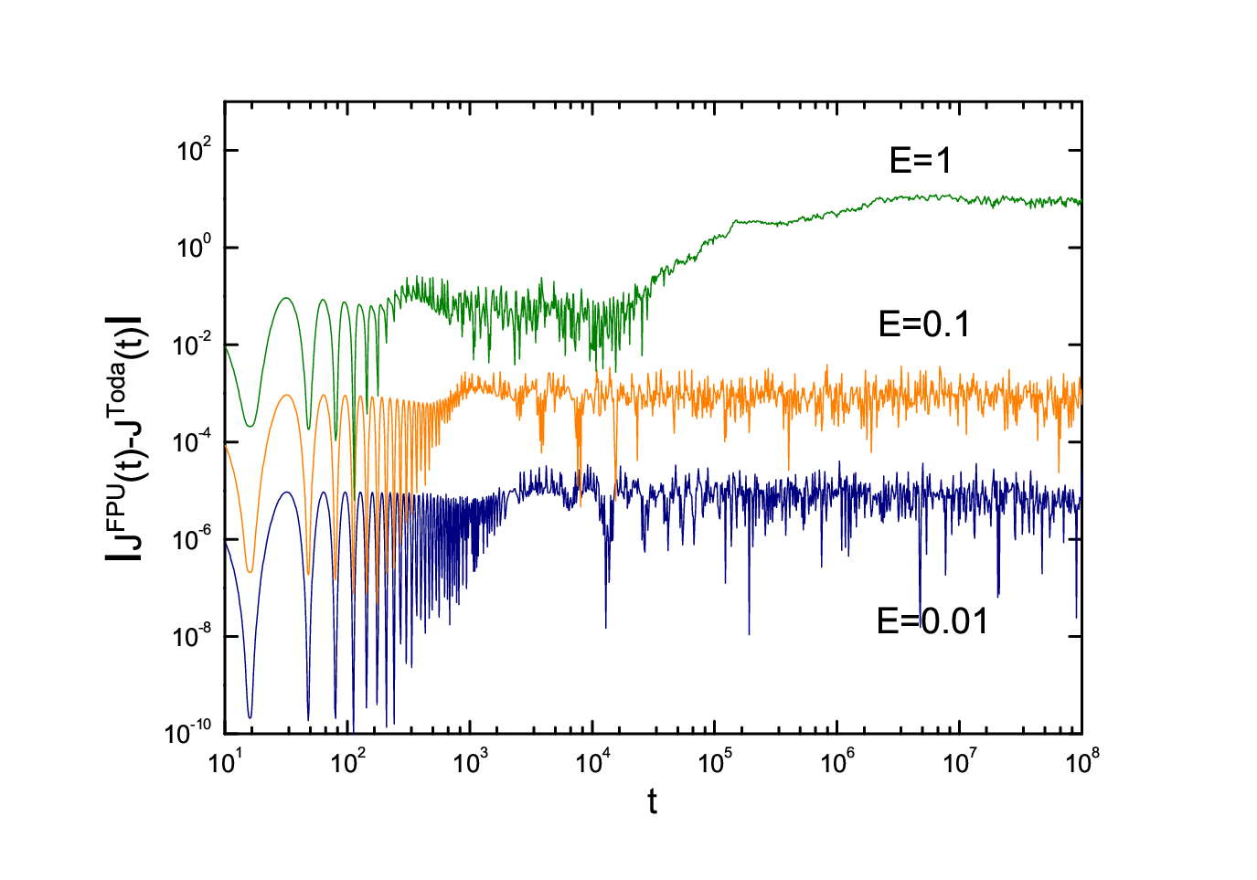
We have studied the evolution of one of the additional constants of motion of the Toda model. The integral we considered is [23]
| (22) |
where () are the Flaschka variables [24], with boundary conditions , , inherited by the restriction of the -periodic case to that of fixed ends. Since is an integral of the Toda model, along the Toda flow. Along the FPU flow the quantity is expected to be small in the perturbative regime where the two models can be considered to be close to each other. Let us denote by and by the evolution of the quantity (22) along the numerical FPU and Toda trajectories, respectively.
In Fig. 9 the absolute error vs. is reported, for the three different values of the energy (bottom to top), in log-log scale. After a transient time, the error stabilizes quickly at a practically constant value ranging from at to at . Thus the numerical algorithm reproduces the integrable Toda dynamics with very good accuracy.
In Fig. 10 we plot the evolution of , for the same three values of the energy (bottom to top), in log-log scale. For or this difference stays almost constant (up to the final observation time ), while for it starts to grow at about to eventually saturate at a constant value. Therefore at low energies the FPU system can be regarded as a perturbation of the Toda one, the exact integrals of the latter being adiabatic invariants, or quasi-integrals, of the former. Note that at and no effective tendency to equipartition was observed up to . On the other hand, for the tail of the FPU m.e.s. starts to effectively raise at , when the drift of the Toda integral starts up.
4 Theory
Our theoretical approach is based on Hamiltonian perturbation theory. We construct a resonant normal form Hamiltonian of the FPU and Toda systems. The laws (11)-(12) are then derived by solving the normal form equations, to leading order, for short times. The law (16) is instead obtained as the m.e.s. of a time-periodic solution of the normal form equations. The theoretical explanation of the diffusion law (20) goes beyond our present capabilities.
4.1 Complex modal variables
Let us consider the Hamiltonian (1) of the FPU -model. We first perform a change of variables passing from the real space coordinates to the complex modal variables . The complex modal variables are defined in terms of the real ones by
| (23) |
whose utility is self-explanatory. The FPU Hamiltonian (1), when expressed in the new complex variables , reads
| (24) |
where a superscript asterisk denotes complex conjugation, and the mode-coupling coefficient
| (25) |
has been introduced ( is the usual Kronecker symbol). We also recall that
| (26) |
denotes a small parameter in the theory. In (24) we have explicitly pointed out the quadratic part and the cubic part of the Hamiltonian. The Hamilton equations of motion associated to the Hamiltonian explicitly read
| (27) |
Finally, the initial condition (2) expressed in the new variables reads
| (28) |
4.2 Averaging
The initial condition (28), at low energy, is expected to excite an oscillation of the first mode at a frequency close to the unperturbed one, the difference vanishing as . Indeed, in the latter limit, equations (27) become linear and are solved by . Now, by substituting the leading order ansatz in the right hand side of equations (27), and making use of (25), one realizes by a direct inspection that the mode is forced, among others, by a term oscillating at a frequency . Thus, mode responds close to resonance and its amplitude grows, which requires to modify the starting ansatz to . Re-inserting the latter in the right hand side of (27) one finds that mode is almost resonantly pumped at a frequency , and so on. Such a process leads to an almost resonant transfer of energy from the fundamental mode to higher frequency modes, with mode oscillating at the frequency . For this reason, we perform the time-dependent change of variables
| (29) |
for . The above defined map is actually the -periodic flow of the Hamiltonian
| (30) |
Notice also that all the functions of the modal energies , such as and , are invariant under the flow , i.e. Poisson-commute with . The new variables evolve according to the Hamilton equations associated to the explicitly time-dependent, -periodic Hamiltonian :
| (31) |
According to the usual averaging theory [46, 47], we replace the explicitly time-dependent Hamiltonian with its time average . This amounts to replacing , on the right hand side of (31), with its time average
| (32) |
We then obtain an averaged system, whose solution stays close to that of the original system over times inverse proportional to the small parameter. The averaged Hamiltonian of the system then reads
| (33) |
and its associated Hamilton equations read
| (34) |
where, if or , the first or the second sum on the right hand side are respectively absent. Such equations must be solved, for , with the initial condition
| (35) |
4.3 Solution of the averaged system
The averaged equations (34) contain the small parameter . We set
| (37) |
the dependence on being left in the nonlinear frequency shift . We require that as , so that in absence of nonlinearity the initially excited mode will oscillate with its unperturbed frequency . It follows[48]
| (38) |
| (39) |
The initial condition implies
| (40) |
Upon substitution of (38)-(39) in (34) and balancing order by order one gets a nonlinear system of coupled equations at any order . The first two orders () explicitly read:
| (41) |
| (42) | |||||
Again, a sum is absent if the upper limit of summation is less than one. The latter two systems, in which the unknowns are , and , have a triangular structure, i.e. the equations can be solved one after the other starting from the first down to the last one, with the initial condition (40). The expansion of the frequency shift (39) (i.e. the coefficients ) is determined by requesting the vanishing of possible secular terms in the expansion of . One thus arrives at the following leading order expansions:
| (43) |
| (44) |
| (45) |
| (46) |
the dots standing for terms of higher order.

In Fig. 11 the first four modal energies of the -model are plotted vs. time , in log-log scale, at the energy value . The red curves represent the numerical values, while the four black lines correspond to the three analytic formulae (44)-(46) and to that of mode , which is not explicitly reported here, since it has a very long, uninteresting expression. Note that . Note how the agreement is excellent up to the final computation time .
Fig. 11 shows that the perturbative scheme used here works very well at low energies. The regime of validity of the perturbative solution can be estimated by requiring that in the expansions (43) and (44) of and of the , respectively, the leading order is dominant with respect to the correction proportional to . The latter condition turns out to be more restrictive than the former and, by taking into account that , yields
| (47) |
i.e. an upper bound to the energy which decreases with increasing . For and , one gets . Using (43), condition (47) can be transformed into
| (48) |
Thus the ratio of the nonlinear frequency shift to the resonance width must be smaller than a constant, which is akin to the so-called resonance overlap criterion first formulated in Ref. [49] (notice that in the latter paper, dealing with the FPU- model, the considered resonance width was different; see also Refs. [9] and [11] for comments on this point).
For values of the energy larger than about the agreement of the expressions (44)-(46) with the numerical data starts to worsen, and one would really need to include higher order corrections. However, some leading order analytic predictions concerning the behavior of the ’s can still be obtained, within the same perturbative scheme, either on very short times, or at saturation, as follows.
4.4 Secular avalanche
Since by the initial condition (40) all the are zero at if and is small for low modes (and exactly vanishes for ), the contribution to the short term dynamics coming from the linear term on the right hand side of the equations (41) is expected to be small on short time. By neglecting such a term the leading order equations (41) simplify to
| (49) |
where again the sum on the right hand side is absent for . Equations (49) with the initial condition admit the exact (unique) solution
| (50) |
where the coefficients are computed by solving the nonlinear map
| (51) |
for . Notice that to leading order, the first mode does not change from the initial condition: . The evolution equation for the first mode at second order can be obtained by solving the second order equations (42) for with the choice .[50] Taking into account that , and making use of (50) and (51) to get and , one gets a differential equation for , which can be integrated with the initial condition . The result is
| (52) |
Finally, the normalized modal energies can be computed:
| (53) |
| (54) |
which explains the derivation of the law (11)-(12) reported in Section II and tested in Fig. 2 of Section III.
4.5 Role of resonance detuning and energy conservation
Let us discuss the validity of the approximation obtained by neglecting the linear term on the right hand side of equations (41). This is done by substituting on the right hand side of the same equation the solution (50) and by checking whether and how long the linear term stays smaller than the quadratic term. One thus finds that a first necessary condition for the approximation to be valid is that
| (55) |
The detuning time is the characteristic time within which mode is resonantly pumped, the term proportional to the resonance amplitude being negligible. Now, is a monotonically decreasing function of , and for high mode numbers , whereas for low modes , which can be as large as for the first few modes, actually too large to be compatible with the observed time-scale of formation of the quasi-state. When checking the validity of the approximation made by neglecting the linear term in (41), one has to take into account that the quantity , defined in (36), is constant and equal to one. The latter condition implies that for any , yielding, when the (approximate) solution (50) is taken into account, a second necessary condition for the validity of the approximation made, namely
| (56) |
is the mode dependent characteristic time of the secular avalanche process, i.e. the time within which mode can grow, when resonantly pumped by the cascade process, without violating the conservation of the energy . We find that is a monotonically decreasing function of and, by direct inspection of the map (51), that , if is not too small. Note that from (53) it follows that if , while there is obviously no detuning time for the first mode.
Having two characteristic times for each mode , namely and , the actual characteristic time at which stops its secular growth is defined as the minimum of the two for each : . For small values of , for and for . An order of magnitude estimate of is obtained by observing that for almost all modes, whereas if (numerical factors are neglected). Then the crossover takes place at the critical mode number
| (57) |
valid if , i.e. if . The time-scale for the formation of the quasi-state is defined as the crossover time at :
| (58) |
which is the estimate (15).
From the above reasonings, it follows that modes with are always inside a resonance layer and their modal energies stop to grow due to energy conservation, whereas modal energies with stop to grow due to resonance detuning. We thus distinguish core modes with from those with . Core modes share most of the energy in the quasi-state, and the resonant transfer of energy among them is effective. Higher modes outside the core are resonantly pumped for a certain time and are tuned out of resonance rather quickly. The quasi-state is characterized by a few core modes sharing the energy and by an exponential localization of the m.e.s. for high modes. Notice that for and , equation (57) gives varying from to as the energy varies from to , in agreement with the number of modes that define the plateau of partial equipartition observable in the numerical spectra reported in the left column of Fig. 3.
4.6 Fixed point of the averaged system: quasi-state
Let us consider the averaged equations (34). In the limit one has , we require , and the equations simplify to
| (59) |
whose solution with initial condition (35) is . In other words, the system is placed at on a fixed point and stays there forever. Notice that system (59) admits a one-parameter family of fixed points
| (60) |
which is a unit circle in the -plane of . It can be easily checked that the set is the maximum of the Hamiltonian (limit of the Hamiltonian as ) constrained to the set . If but small enough, the set is slightly deformed to the set of stationary points of the full averaged system (34) on the set , i.e. the set of critical points of the Hamiltonian constrained to the set . Moreover, if is small enough, the critical set preserves its maximum property (i.e. is the maximum of on ) and turns out to be Lyapunov stable: if is initially close to it stays close to it forever. On the other hand, the initial condition means that one starts on , so that if and are close, i.e. if is small enough, the orbit of the averaged system stays forever close to . We make use of this qualitative (but exact) reasoning to identify the quasi-state orbit of the -model with the set .
The fixed points of system (34) can be perturbatively computed by means of the expansions (38)-(39). To leading order, one has to find the fixed point of system (41), setting , which yields
| (61) |
where , at this stage, is an arbitrary complex number such that , to leading order. Isolating the dependence of on one gets
| (62) |
where the real coefficients are found by solving the nonlinear map problem
| (63) |
for . Recalling that, to leading order, , one can compute the m.e.s.
| (64) |
Such a spectrum depends on the unknown , which is determined by the normalization condition , i.e.
| (65) |
The latter condition determines the modulus of , so that an overall phase remains undetermined. For this reason, the set is composed by a one-parameter family of stationary points of the averaged system.
We now observe that to a stationary solution of the averaged system, there corresponds a periodic orbit, or one-dimensional torus, of the original system: recall that, before averaging, we performed the change of variables . The fundamental frequency of the quasi-state periodic orbit is easily determined by means of equations (42). Setting there and , and making use of (62)-(63), one gets
| (66) |
which implies
| (67) |
Notice that in the regime of strong localization, when , the above expression for the corrected frequency coincides with that given in (43).
As already mentioned, the quasi-state m.e.s. (64) fits the numerically obtained one at low energy, when the exponential localization is so strong that only a few low modes contribute to the total energy. In this case, the map (63) can be approximately solved, as follows. First of all, notice that if only low (acoustic) modes are relevant, one can substitute the approximate expressions , in the numerator and denominator of (63), respectively. Second, we look for a solution of the map in the form , which fits the condition . Upon substitution of the latter expression into (63), and after some simple calculation, one gets . Thus, in the regime of strong localization, the approximate solution of the map (63) is given by . As a consequence, recalling that and that , for the spectrum (64) one gets the approximate expression
| (68) |
Under the same acoustic approximation () leading to the latter formula, condition (65) becomes
| (69) |
This explains formulas (16)-(18) given in Section II. We stress again that the m.e.s. (68) corresponds to the leading order spectrum of the Lyapunov continuation to the nonlinear case of the first mode, first reported in Ref. [5] and there named -breather. We also recall here that the normalization condition (69) can be simply solved. Indeed, by defining and , it is easily found that (69), in the limit of large and for , yields the simple implicit equation . This is explicitly solved, for (and ), to give , for a suitable function , which determines (and thus ) in terms of the total energy , of and of the number of particles . In particular, having determined , it turns out that, at any fixed , , which can then be used to finally determine the m.e.s. (68).
To conclude this subsection, we observe that all the above construction was performed to leading order, and applied to the Toda model, would give the same result. This is a consequence of the coincidence to third order of the FPU- and the Toda models expressed by relation (4).
4.7 Long term stability of the quasi-state
The argument used to guess that the one parameter family of stationary points of the Hamiltonian (33) constrained to the set is the candidate quasi-state orbit of the FPU- and Toda models, is a qualitative one. We did not specify how small the parameter has to be to ensure that is a maximum of the constrained averaged Hamiltonian and moreover the unperturbed orbit (which contains the initial datum) is in the domain of concavity of . In this respect, we do not provide any precise estimate on , which would require technical arguments that are beyond the aim of the present paper. We only mention that, from the discussion made in Section IV C above, one may expect that a condition of the form should hold to ensure the Lyapunov stability of .
Apart from the precise energy-size dependence of the stability domain of the one-dimensional torus , it is important to understand that the construction made above is a leading order one, which ensures, for the real system, confinement close to the set on a relatively short time-scale, typically an inverse power law of the small parameter . In order to explain the stability on much longer times observed numerically, one should go beyond the leading order construction, which modifies the averaged Hamiltonian (33) with the addition of higher order terms, and increases the length of the confinement time. Such an approach was used in Refs. [51, 52, 53] to prove that in the case of initial excitation of the first mode in a suitable class of string equations, the confinement time grows as the exponential of the inverse of the small parameter. However, it must be stressed that importing those techniques to the problem at hand is nontrivial at all, essentially due to the lack of complete resonance in the FPU problem (explicit reference to the FPU problem, in this perspective, has been made in Ref. [52]).
5 Concluding remarks
We have shown that the classical FPU paradox can be easily understood if one compares the behavior of the (presumably) nonintegrable FPU--model with that of the integrable Toda model, for the same initial condition, at the same energy. One thus finds that the dynamics of the -model on a short initial time interval is very close to that of the Toda model. The quasi-state guessed by FPU is nothing but the quasi-periodic Toda torus on which the dynamics is initiated for the same initial condition. At very low energy, such a torus becomes one-dimensional and the FPU- system evolves close to it up to extremely long times. As the energy increases, the dimension of the reference torus grows, while the time of confinement close to it (or stability time) for the FPU- system decreases. Finally, the approach to a state of energy equipartition of the FPU- model takes place through a diffusive-like detachment from the quasi-state, a phenomenon that is chaotic in character, and consequently, absent in the integrable model.
Regarding the FPU -model as a perturbation of the Toda one, as first suggested in Ref. [16], and strongly motivated here, seems to be quite promising. For example, in Ref. [54] it is shown that the Toda Hamiltonian fits the hypotheses requested to the unperturbed Hamiltonian in the Nekhoroshev theorem, with the purpose to explain the phenomenology of the FPU- model in terms of the exponential stability of all the Toda integrals (or actions). However, precise/optimal estimates of the regime of validity (energy-size domain) of such a conclusion are still lacking. Of course, if the energy is small enough, one cannot exclude the possibility to enter a KAM regime, i.e. to have stability over infinitely long times. Here also, we know that this is possible in principle[55], but again, precise/optimal estimates of the regime of validity are not available yet. We finally notice that it is not presently clear whether this approach (i.e. considering the FPU system as a perturbation of the Toda one) is valid for initial conditions involving also high frequency modes or even for generic excitations.
One interesting question is whether and how the energy region for the long-term stability of the quasi-state collapses or not to zero by increasing . In the light of the purely numerical results contained in Ref. [28], a first answer seems to be that exponentially long times to equipartition might be, for the -model, a finite-size effect, observable only in an unspecified regime as . In the same paper, it is shown that for particular low frequency initial data, the -model seems to exhibit exponentially long times to equipartition in the thermodynamic limit. On the other hand, in Ref. [56], an analytic lower bound to the canonical mixing time of a weakly coupled model is provided, showing that such time is longer than a stretched exponential of the inverse of the temperature. The full scenario is quite complicated and deserves a lot of further study.
acknowledgments
This work was initiated and in large part completed during a stay of A.P. and H.C. in the MPIPKS of Dresden, whose facilities were used to perform all the numerical calculations. The authors thank D. Bambusi, G. Benettin, A. Giorgilli and T. Penati for useful discussions on the subject, and are also indebted to D. Ryabov for important remarks on the Toda model.
References
- [1] E. Fermi, J. Pasta and S. Ulam, LA-1940 internal report, 1955. Reprinted in the Collect Papers of E. Fermi, Vol. II, University of Chicago Press and Accademia Nazionale dei Lincei, 1965, 978-988.
- [2] E. Fucito, F. Marchesoni, E. Marinari, G. Parisi, L. Peliti, S. Ruffo and A. Vulpiani, J. de Phys. 43, 707-713 (1982).
- [3] R. Livi, M. Pettini, S. Ruffo and A. Vulpiani, Phys. Rev. A 31, 2740-2742 (1985).
- [4] L. Berchialla, L. Galgani and A. Giorgilli, DCDS-A 11, 855-866 (2004).
- [5] S. Flach, M. V. Ivanchenko and O. I. Kanakov, Phys. Rev. Lett. 95, 064102/1-4 (2005).
- [6] S. Flach, M. V. Ivanchenko and O. I. Kanakov, Phys. Rev. E 73, 036618/1-14 (2006).
- [7] S. Flach, O. I. Kanakov, M. V. Ivanchenko and K. G. Mishagin, Int. J. Mod. Phys. B 21, 3925-3932 (2007).
- [8] T. Penati and S. Flach, Chaos 17, 023102/1-16 (2007).
- [9] S. Flach and A. Ponno, Physica D 237, 908-917 (2008).
- [10] N. J. Zabusky and M. D. Kruskal, Phys. Rev. Lett. 15, 240-243 (1965).
- [11] D. L. Shepelyansky, Nonlinearity 10, 1331-1338 (1997).
- [12] A. Ponno, Europhys. Lett. 64, 606-612 (2003).
- [13] A. Ponno, in Chaotic Dynamics and Transport in Classical and Quantum Systems, P. Collet et al. (eds.); Kluwer Academic Publishers, 431-440 (2005).
- [14] D. Bambusi and A. Ponno, Commun. Math. Phys. 264, 539-561 (2006).
- [15] G. Benettin, R. Livi and A. Ponno, J. Stat. Phys. 135, 873-893 (2009).
- [16] W. E. Ferguson Jr., H. Flaschka and D. W. McLaughlin, J. Comp. Phys. 45, 157-209 (1982).
- [17] S. Isola, R. Livi, S. Ruffo and A. Vulpiani, Phys. Rev. A 33, 1163-1170 (1986).
- [18] L. Casetti, M. Cerruti-Sola, M. Pettini and E. G. D. Cohen, Phys. Rev. E 55, 6566-6574 (1997).
- [19] A. Giorgilli, S. Paleari and T. Penati, DCDS-B 5, 991-1004 (2005).
- [20] N. J. Zabusky, Z. Sun and G. Peng, Chaos 16, 013130/1-12 (2006).
- [21] M. Toda, Phys. Rep. 18, 1-124 (1975).
- [22] J. Ford, S. D. Stoddard and J. S. Turner, Prog. Theor. Phys. 50, 1547-1560 (1973).
- [23] M. Hénon, Phys. Rev. B 9, 1921-1923 (1974).
- [24] H. Flaschka, Phys. Rev. B 9, 1924-1925 (1974).
- [25] M. Pettini and M. Landolfi, Phys. Rev. A 41, 768-783 (1990).
- [26] J. De Luca, A. J. Lichtenberg and S. Ruffo, Phys. Rev. E 60, 3781-3786 (1999).
- [27] L. Berchialla, A. Giorgilli and S. Paleari, Phys. Lett. A 321, 167-172 (2004).
- [28] G. Benettin and A. Ponno, J. Stat. Phys. 144, 793-812 (2011).
- [29] J. Ford, Phys. Rep. 213, 271-310 (1992).
- [30] Focus Issue The “Fermi-Pasta-Ulam”-problem: the first 50 years, Chaos 15 (2005).
- [31] The Fermi-Pasta-Ulam Problem: A Status Report, Lect. Notes Phys. 728, G. Gallavotti ed.; Springer-Verlag, 2008.
- [32] H. Yoshida, Phys. Lett. A 150, 262-268 (1990).
- [33] H. Yoshida, Cel. Mech. Dyn. Astron. 56, 27-43 (1993).
- [34] The time-step must be much smaller than , the latter being the minimum normal mode period (the maximum frequency is ). The fourth order algorithm ensures energy conservation with an absolute error of the order . For details on the numerical integration of FPU systems see e.g.: G. Benettin and A. Ponno, Physica D 240, 568-573 (2011).
- [35] The value of is irrelevant, since it can be set to one by the canonical transformation , which also shows that the actual parameter of nonlinearity in the problem is the product .
- [36] Formula (8) can be obtained by first computing for the initial condition (2), expanding the exponential in the Toda potential (3), and then summing first over .
- [37] M. Abramowitz and I. A. Stegun, Handbook of Mathematical Functions, Dover, 1965.
- [38] In the regime explored in the present paper , or, which is the same, . Indeed, since , from (7) and (8) it follows that , and the quantity is always small in our runs, being at most down to , and even lower in some cases.
- [39] Since the cubic potential is not lower bounded, the micro-canonical measure of the -model does not exist and the system breaks-down in a finite time when a sufficient amount of energy localizes on a few particles. As a matter of fact, in the quasi-linear regime considered here, the break-down takes place after equipartition has been reached, the latter state being well described by the micro-canonical measure of the harmonic chain. In all the numerical runs reported in the sequel the break-down was never reached.
- [40] J. Ford, J. Math. Phys. 2, 387-393 (1961).
- [41] R. Livi, S. Ruffo, M. Pettini and A. Vulpiani, Il Nuovo Cimento B 89, 120-130 (1985).
- [42] N. J. Zabusky, J. Math. Phys. 3, 1028-1039 (1962).
- [43] M. D. Kruskal and N. J. Zabusky, J. Math. Phys. 5, 231-244 (1964).
- [44] H. Christodoulidi, C. Efthymiopoulos and T. Bountis, Phys. Rev. E 81, 016210/1-16 (2010).
- [45] H. Christodoulidi, C. Efthymiopoulos and T. Bountis; preprint (2011).
- [46] N. N. Bogolyubov and Y. A. Mitropolsky, Asymptotic Methods in the Theory of Non-linear Oscillations, Gordon & Breach, NY, 1961.
- [47] J. A. Sanders, F. Verhulst and J. Murdock, Averaging Methods in Nonlinear Dynamical Systems, Springer, 2007.
- [48] As can be proved by induction, (38) and (39) are the only possible formal power series expansions compatible with the equations (34) and with the initial condition (35).
- [49] F.M. Izrailev and B.V. Chirikov, Sov. Phys. Dokl. 11, 30-34 (1966).
- [50] The quantity is an unknown of the problem and there is more than one way to determine its value; by setting the latter value to zero means giving up to control secular divergencies, which still yields an approximate solution, though valid over very short times.
- [51] D. Bambusi and N. N. Nekhoroshev, Physica D 122, 73-104 (1998).
- [52] N. N. Nekhoroshev, in the Proceedings of the Porquerolles School 2001 on Hamiltonian Systems and Fourier Analysis, ed. by D. Benest et al., Cambridge Scientific Publishers, 289-302 (2005).
- [53] N. N. Nekhoroshev, Trans. Moscow Math. Soc. of the year 2002, 151-217.
- [54] A. Henrici and T. Kappeler, Chaos 19, 033120/1-13 (2009).
- [55] B. Rink, Commun. Math. Phys. 261, 613-627 (2006).
- [56] A. Carati and A. Maiocchi; preprint (2010) on http://arxiv.org/abs/1011.5846