(In-)Stability of singular equivariant solutions to the Landau-Lifshitz-Gilbert equation
Abstract
In this paper we use formal asymptotic arguments to understand the stability properties of equivariant solutions to the Landau-Lifshitz-Gilbert model for ferromagnets. We also analyze both the harmonic map heatflow and Schrödinger map flow limit cases. All asymptotic results are verified by detailed numerical experiments, as well as a robust topological argument. The key result of this paper is that blowup solutions to these problems are co-dimension one and hence both unstable and non-generic.
Finite time blowup solutions are thus far only known to arise in the harmonic map heatflow in the special case of radial symmetry. Solutions permitted to deviate from this symmetry remain global for all time but may, for suitable initial data, approach arbitrarily close to blowup. A careful asymptotic analysis of solutions near blowup shows that finite-time blowup corresponds to a saddle fixed point in a low dimensional dynamical system. Radial symmetry precludes motion anywhere but on the stable manifold towards blowup.
The Landau-Lifshitz-Gilbert problem is not invariant under radial symmetry. Nevertheless, a similar scenario emerges in the equivariant setting: blowup is unstable. To be more precise, blowup is co-dimension one both within the equivariant symmetry class and in the unrestricted class of initial data. The value of the parameter in the Landau-Lifshitz-Gilbert equation plays a very subdued role in the analysis of equivariant blowup, leading to identical blowup rates and spatial scales for all parameter values. One notable exception is the angle between solution in inner scale (which bubbles off) and outer scale (which remains), which does depend on parameter values.
Analyzing near-blowup solutions, we find that in the inner scale these solution quickly rotate over an angle . As a consequence, for the blowup solution it is natural to consider a continuation scenario after blowup where one immediately re-attaches a sphere (thus restoring the energy lost in blowup), yet rotated over an angle . This continuation is natural since it leads to continuous dependence on initial data.
Keywords: Landau-Lifshitz-Gilbert, Harmonic map heatflow, Schrödinger map flow, asymptotic analysis, blowup, numerical simulations, adaptive numerical methods
1 Introduction
In this paper we are interested in the existence and stability of finite-time singularities of the Landau-Lifshitz-Gilbert equation for maps from the unit disk (in the plane) to the surface of the unit sphere, :
| (1) |
We will always require the damping term and take without loss of generality. This problem preserves the length of the vector , i.e., for all implies that for all positive time (for all ).
In the case this equation arises as a model for the exchange interaction between magnetic moments in a magnetic spin system on a square lattice [20, 21]. Taking recovers the harmonic map heatflow which is a model in nematic liquid crystal flow [8]. It is also of much fundamental interest in differential geometry [27]. Finally, the conservative case is the Schrödinger map from the disk to the sphere, which is a model of current study in geometry [12, 16, 17].
Stationary solutions in all these cases are harmonic maps. This allows us to analyze singularity formation in a unified manner for all parameter values. Traditionally, the Landau-Lifshitz-Gilbert equation is posed with Neumann boundary conditions, but this does not affect the local structure of singularities, should they arise. We note that in the harmonic map literature the second term on the right-hand side of the differential equation (1) is often rewritten using the identities
where denotes the inner product in and , with the components of .
As discussed in much greater detail in Sections 1.1 and 1.2, there are initial data for which the solution to (1) becomes singular in finite time. In this paper we analyze this blowup behaviour, in particular its stability properties under (small) perturbations of the initial data. Considering initial data that lead to blowup, the question is whether or not solutions starting from slightly different initial data also blowup. Our main conclusion is that blowup is an unstable co-dimension one scenario. With this in mind we also investigate the behavior of solutions in “near-miss” of blowup, and the consequences this has for the continuation of the blowup solution after its blowup time.
1.1 Problem formulation
We will consider two formulations for equation (1). The first is the so-called equivariant case: using polar coordinates on the unit disk , these are solutions of the form
| (2) |
which have the (intertwining) symmetry property for all and each fixed , where is a rotation over angle around the origin in the plane , while is a rotation over angle around the -axis in .
The components then satisfy the pointwise constraint , as well the differential equations
| (3) |
where
We will take in what follows, except in Section 6.
Alternatively, we can parametrize the solutions on the sphere via the Euler angles:
| (4) |
where the equations for and are given by
| (5) |
We note that due to the splitting in (4) the system (5) has one spatial variable. In this equivariant case the image of one radius in the disk thus fixes the entire map (through rotation) and we write .
In the special case and only, there are radially symmetric solutions of the form constant, reducing the system to a single equation
| (6) |
1.2 Previous results
It is well known that not all strong solutions to the radially symmetric harmonic map heatflow (6) are global in time. Equation (6) is -periodic in . Supplemented with the (finite energy) boundary condition , it only has stationary solutions of the form for . Hence with prescribed boundary data and there is no accessible stationary profile. However, there is an associated Lyapunov functional,
whose only stationary points are the family . It is this paradox that leads to blowup: there is a finite collection of (possibly finite) times at which “jumps” from to , losing of energy [27, 6]. The structure of the local solution close to the jumps (in time and space) is known, which allows us to analyze the stability of these solutions.
The fundamental result in this area is due to Struwe [27] who first showed that solutions of the harmonic map heatflow could exhibit the type of jumps described above and derived what the local structure of the blowup profile is. Chen, Ding and Ye [11] then used super- and sub-solution arguments, applicable only to (6), to show that finite-time blowup must occur when and . The blowup rate and additional structural details were determined through a careful matched asymptotic analysis in [29].
The analysis is based on the original result of Struwe who showed that any solution which blows up in finite time must look locally (near the blowup point) like a rescaled harmonic map at the so-called quasi-stationary scale. That is, there is a scale on which the solution takes the form
| (7) |
From [29] it is known that for generic initial data one has
| (8) |
for some and blowup time , which both depend on the initial data. This result is intriguing as the blowup rate is very far from the similarity rate of [3].
While the blowup rate (8) was derived in [29] for the harmonic map heatflow, i.e. , , in this paper we demonstrate that formal asymptotics imply that this rate is universal for all parameter values of and . Very recently, proofs of the blowup rate (8) have appeared for the harmonic map heatflow [24] as well as the Schrödinger map flow [23], i.e., the two limit cases of the Landau-Lifshitz-Gilbert problem.
It is common to consider radial symmetry when analyzing the blowup dynamics of many reaction-diffusion equations. Typically there one can show that there must be blowup using radially symmetric arguments. Moreover, numerical experiments generically show that rescaled solutions approach radial symmetry as the blowup time is approached.
For the harmonic map problem the proof of blowup solutions due to Cheng, Ding and Ye is completely dependent on the radial symmetry. Moreover, there are stationary solutions to the problem which are in the homotopy class of the initial data, but which are not reachable under the radial symmetry constraint. This begs the question: What happens when we relax the constraint of radially symmetric initial data?
The above description is mainly restricted to the harmonic map problem () which has received considerably more attention than the general Landau-Lifshitz-Gilbert equation. Before addressing the question of stability under non-radially symmetric constraints for the harmonic map heatflow problem, we first show that blowup solutions are still expected for the full Landau-Lifshitz-Gilbert equation with , see Section 2. We note that
is a Lyapunov functional for the equivariant problem (5) as long as , whereas it is a conserved quantity for the Schrödinger map flow ().
We discuss the question of stability for the full problem in a uniform manner. The topological argument in Section 2 suggests that blowup is co-dimension one, and this is indeed supported by the asymptotic analysis in Section 3 and the numerics in Section 4. The main quantitative and qualitative properties turn out to be independent of the parameter values, except for the angle between sphere that bubbles off and the remaining part of the solution. In Section 5 we analyze near-blowup solutions. These solution rotate quickly over an angle in the inner scale. For the blowup solution this implies a natural continuation scenario (leading to continuous dependence on initial data) after the time of blowup: the lost energy is restored immediately by re-attaching a sphere, rotated over an angle . Finally, in Section 6 we present the generalization to the case , followed by a succinct conclusion in Section 7.
2 The global topological picture
We present a topological argument to corroborate that blowup is co-dimension one. It does not distinguish between finite and infinite time blowup. Since the argument relies on dissipation, it works for , but since the algebra is essentially uniform in and , as we shall see in Section 3, we would argue that the situation for the Schrödinger map flow is the same.
Let us first consider the equivariant case, where, as explained in Section 1.1, the image of one radius in the disk fixes the entire map, and we write .
Let (the north pole) and . In the notation using Euler angles from Section 1.1, by rotational symmetry we may assume that , . The only equilibrium configuration satisfying these boundary conditions is , where . Note that for there is no equilibrium, hence blowup must occur for all initial data in that case [2].
For , i.e. , we shall construct a one parameter family of initial data , and we argue that at least one of the corresponding solutions blows up. Since the presented argument is topological, it is robust under perturbations, hence it proves that blowup is (at most) co-dimension one. The matched asymptotic analysis in Section 3 confirms this co-dimension one nature of blowup.
We choose one-parameter families of initial data as follows. The family of initial data will be parametrized by , or with the end points identified. Let be a continuous map from to , such that
| (9) |
We may then view as a map from by identifying and to points. Now choose any continuous family satisfying (9) such that it represent a degree 1 map from to itself. One such choice is obtained by using the stereographic projection
Let be such that , i.e. . Then we choose
see also Figure 1. For the special case that we choose
| (10) |
This is just one explicit choice; any homotopy of this family of initial data that obeys the boundary conditions (9) also represents a degree 1 map on . Let be the collection of initial data obtained by taking all such homotopies. It is not hard to see that is the space of continuous functions (with the usual supremum norm) satisfying the boundary conditions. Let be the subset of initial data in for which the solution to the equivariant equation (3) blows up in finite or infinite time. The following result states that the co-dimension of is at most one. In particular, each one parameter family of initial data that represent a degree 1 map from to itself has at least one member that blows up.
Proposition 1.
Let . The blowup set for the equivariant equation (3) has co-dimension at most 1.
Proof.
Let be any family of initial data that, via the above identification, represent a degree 1 map from to itself. Let correspond to the solution with initial data . As explained above, we see from (9) that we may view as a map from by identifying and to points. Since the boundary points are fixed in time, we may by the same argument view as a map from to itself along the entire evolution. Note that since the energy is a Lyapunov functional for , any solution tends to an equilibrium as . If none of the solutions in the family would blow up (in finite or infinite time) along the evolution, then all solutions converge smoothly to the unique equilibrium. In particular, for large the map has its image in a small neighborhood of this equilibrium, hence it is contractible and thus has degree 0. Moreover, if there is no blowup then is continuous in , i.e. a homotopy. This is clearly contradictory, and we conclude blowup must occur for at least one solution in the one-parameter family . This is a topologically robust property in the sense that any small perturbation of also represents a degree 1 map, and the preceding arguments thus apply to such small perturbations of as well. This proves that the co-dimension of is at most 1. ∎
One may wonder what happens when (equivariant) symmetry is lost. Although a priori the co-dimension could be higher in that case, we will show that this is not so. For convenience, we only deal with boundary conditions for all , which simplifies the geometric picture, but the argument can be extended to more general boundary conditions.
The only equilibrium solution in this situation is [22]. Let be the family of initial data for the equivariant case with boundary condition (see (10) and Figure 1). Consider now the following family of initial data for the general case:
We see that maps to , and , but also . We may thus identify to a point, and interpret as a map from to . In particular, represents an element in the homotopy group . Furthermore, upon inspection, represents the generator of the group, since it is (a deformation of) the Hopf map (see e.g. [18]). Let be the collection of initial data in one parameter families obtained from all homotopies of that obey the boundary conditions
| (11) |
Let be the subset of initial data in for which the solution to the differential equation (1) blows up in finite or infinite time. As before, the co-dimension of is at most 1, showing that dropping the equivariant symmetry does not further increase the instability of the blowup scenario.
Proposition 2.
Let and . The blowup set for the general equation (1) has co-dimension at most 1.
Proof.
The proof is analogous to the one of Proposition 1, but one uses instead of , i.e. the degree, to obtain the contradiction. ∎
As a final remark, even though blowup is co-dimension one, this does not mean it is irrelevant. Clearly, by changing the initial data slightly one may avoid blowup. On the other hand, the arguments above indicate that blowup is caused by the topology of the target manifold, and one can therefore not circumvent this type of singularity formation by simply adding additional terms to the equation (for example a physical effect that works on a smaller length scale), unless additional equilibria are introduced which reflect the pinning of a defect.
3 Asymptotic analysis
In this section we extend the results of [29], where the rate of blowup for radially symmetric solutions to the harmonic heat map problem (6) was determined. We will consider both the extension to the full Landau-Lifshitz-Gilbert equation (i.e. ), as well as allowing a particular class of non-radial perturbations. We find that blowup solutions are always unstable in the equivariant regime. It can be understood that the blowup solutions are separatrices between two distinct global behaviors.
3.1 The inner region
We will proceed with an expansion motivated by two facts: (i) blowup in the harmonic map heatflow is a quasi-static modulated stationary solution; (ii) the full LLG problem has the same stationary profiles as the harmonic map heatflow.
Without specifying the rescaling factor yet we introduce the rescaled variable
which transforms (5) to
| (12) | ||||
To solve this in the limit we pose the expansion
where
| (13) | ||||
| (14) |
represent slow movement along the two-parameter family of equilibria and .
At the next order we have
| (15) | ||||
| (16) |
These equations can both be solved exactly, but we omit the algebraic details since for the matching we only need the asymptotic behaviour as , viz.:
| (17) | ||||||
| (18) |

At this stage both and are unspecified functions. They will be determined through the matching of the inner () and outer regions (), cf. Figure 2.
3.2 The outer region
To make the mechanics of the linearization and matching as transparent as possible we shall now change variables by linearizing around the south pole in the formulation (3):
This recovers
| (19) | ||||
| (20) |
To solve this we introduce , whence
| (21) |
This is simply the projection of the flow from the sphere on to the tangent plane at the pole. Notice that in the respective limits we the recover modified linear heat equation () and Schrödinger equation ( on the tangent plane as appropriate.
To match the inner and outer regions we first define the similarity variables
| (22) |
To reduce confusion in what follows we shall denote
Under this change of variables equation (21) becomes
| (23) |
A solution for this equation is
for any — this is just in (21). This corresponds to the eigenfunction of the dominant eigenvalue of , which governs the generic long time behaviour of solutions of (23). When we allow to vary slowly with , we obtain a series expansion for the solution of the form
| (24) |
We now see that the introduction of non-zero does not affect the procedure for the expansion.
Denoting , we introduce
| (25) | ||||
We recover and through , and expand for small :
| (26) | ||||||
| (27) | ||||||
Here and in what follows one should be slightly careful interpreting all formulae involving the because of multi-valuedness. For future reference we note that
| (28) | ||||||
| (29) |
3.3 The matching
In order to match the inner region to the outer we first write the inner solution in the similarity variables:
| (30) | ||||
| (31) |
The matching procedure now involves setting and such that the expansions (30) and (31) agree with (26) and (27) respectively, to two orders in :
To solve this we set (with algebraic in ), and after rearranging terms we get
| (32) |
Since is defined not to change exponentially fast in , we neglect the terms of . Using the definition of we may simplify (32) to get
| (33) |
Finally, we introduce , so that
| (34) |
which is independent of and . This formulation strongly suggests that the case is not different from the dissipative case . Before solving and studying the system (34) let us recall what its solutions tell us: gives an algebraic correction to the blowup rate, determines the local behaviour of near blowup and describes the amplitude and orientation of the solution in self-similar coordinates, see (28),(29). In order to fully understand blowup, we need to solve for the blowup coordinates and determine their stability.
The blowup solution is represented by for some constant (or , i.e. ), with . In particular, equations (28),(29) show that there is an angle between the sphere bubbling off and the solution remaining at/after blowup, see Figure 3.
By rotating the sphere we may take without loss of generality, i.e. and (note the sign), see (34). The blowup dynamics is described by
| (35) |
and . This equation has general solutions of the form
We can immediately set as this “instability” reflects shifts in the blowup time and hence is not a real instability — this is common to all blowup problems [25]. We note that so that indeed as , and . This implies that , hence for large (cf. Figure 3).
At this stage we have an asymptotic description of the blowup rate and its local structure. Unfortunately, we do not have enough information to determine stability. To more carefully understand the dynamics of this system we need to linearize about this leading order solution to find the subsequent corrections , , and in , , and , respectively. Taking , , , , we get as the system for the next order
| (36) |
which separates into two systems. The first one is (using )
| (37) |
which, using that solves (35), reduces to
the same equation as for , and provides no additional information. The other system is
| (38) |
which can be rewritten as
or, again using that solves (35),
i.e., once again equation (35). The asymptotic behaviour of and is thus given by ()
where the exponentially growing terms show that blowup is unstable (the neutral mode corresponds to a (fixed, time-independent) rotation of the sphere).
4 Numerical computations
To supplement the formal analysis above we now present some numerical experiments in the radial, equivariant and fully two-dimensional cases.
4.1 Numerical methods
To reliably numerically simulate potentially singular solutions to (1) one needs to use adaptivity in both time and space as well satisfy the constraint . For the former, we use adaptive numerical methods as described in [10]. This approach is based on the moving mesh PDE approach of Huang and Russell [19] combined with scale-invariance and the Sundman transformation in time. The expository paper [10] provides many examples of this method being effective for computing blowup solutions to many different problems. For the latter we can either use formulation (3) and use a projection step or regularize the Euler angle formulation (5). We have implemented both and found little difference in efficiency or accuracy and hence will use formulation (3) for all but Example 1 as it directly follows the above asymptotic analysis.
Full two-dimensional calculations have only been performed in the case of formulation (1) and on the unit disk. This latter fact is for numerical convenience and in no way affects the structure of local singularities (should they arise). Here adaptivity was performed using the parabolic Monge-Ampere equation as described in [9]
4.2 Numerical results
In this Section we present a sequence of numerical experiments to validate the results above. For examples 1-3 we used spatial points, the monitor function
and took
as the rescaling between computational time and physical time . Example 4 was computed on a grid using the same monitor functions. Here we took when using form (3) in radial coordinates, when using form (6) and the Cartesian gradient when solving the problem in two dimensions. In one dimension and in two dimensions is the unit disk. In both cases the integral in the monitor function is computed in the physical variables.
Example 1 - the Radial harmonic map
The first example we will consider is equation (6) with initial data
| (39) |
This case has been proven to blowup with known structure [11, 27] and asymptotically calculated rate . Figures 4 and 5 demonstrate the method and show how the adaptive scheme follows the emerging similarity structure in the underlying evolution. Figure 6 shows excellent agreement with the analytical prediction of convergence to the profile with changing over twelve orders of magnitude.
Example 2 - Equivariant Harmonic map
First we reconsider the example above but using equation (3) with the harmonic map case , . We take the same initial as (39) and set
In Figures 7 and 8 we see the same behaviour as observed above. This is not surprising but a reassuring test of the numerics.
We now consider equation (3) with and for a family of initial data determined via stereographic projection
| (40) |
where
which covers the sphere as varies. From the discussion of Section 2 we would expect blowup for a single value of and decay to the stationary solution in all other cases. Figure 9 shows as a function of the parameter for a sequence of values of and initial data (40).
Example 3 - Full Landau-Lifshitz-Gilbert We now consider the full Landau-Lifshitz-Gilbert equation with and . Figure 10 shows snapshots in time for and as well as over time for a sequence of values of in (40). There is no qualitative difference to the case .
Example 4 - Full Landau-Lifshitz-Gilbert in 2 dimensions We now consider the full Landau-Lifshitz-Gilbert equation with and . Figure 11 shows snapshots in time for with initial data (40) and and a small non-radial perturbation. Figure 12 shows snapshots in time for but now we have taken a larger non-radial perturbation of (40) and varied until we had evidence of blowup. Here changes almost four orders of magnitude before the computation halts.
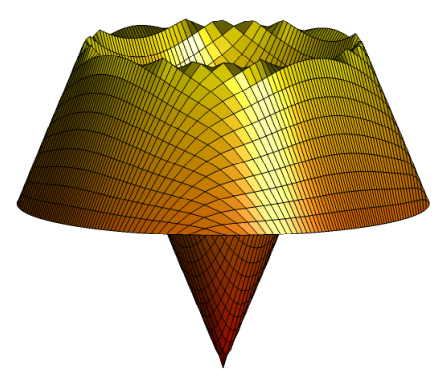
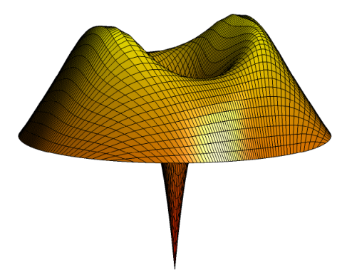
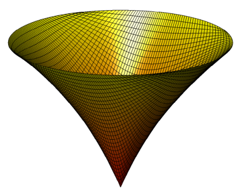
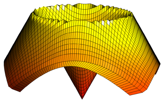
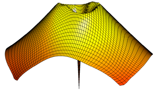
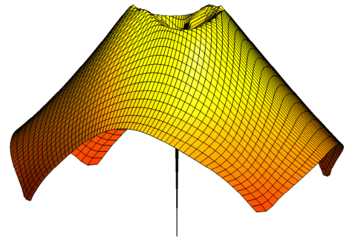
Even though the analysis above is for radial initial data we can find solutions that lead to blowup with carefully tuned parameters specific to given non-radial initial data. This is not necessarily a true blowup solution but rather a numerical one in the sense that it focusses to such a degree that we cannot continue the computation.
5 Behavior of near-blowup solutions
Instability leads to a reconfiguration described by a quick rotation of the sphere that had almost bubbled off. The derivation and asymptotics of this quick rotation are presented in Section 5.1 below. This is highly relevant for the problem of continuing the exceptional solution that does blowup after its blowup time, as explained in Section 5.3.
5.1 The quick rotation
Here we present the asymptotics of near-blowup solutions. The inner scale (in the domain; it describes a sphere in the image, or a semicircle in equivariant coordinates) is given by the usual with
and
For the outer scale (representing a small neighborhood of the south pole in the image) we introduce a fast time scale . On this time scale the dynamics takes place at a small spatial scale , but large compared to , i.e., , where the solution is described by ( representing coordinates in the tangent plane at the south pole as in Section 3.2)
with solution ( and )
Looking at the modulus and argument of we obtain for small
and
Matching to and to , the matching conditions read
In the remote region we have for small for some , where is small close to blowup, as explained in Section 3. And as before, by rotating the sphere we may assume that , with real. By matching it follows that for large , hence and .
Hence, by rearranging the terms we obtain
Let us again remove and from the formulas by setting and . In complex notation: . Furthermore, write . This leads to
Looking at the matching conditions, we write and , with , which we can neglect on this time scale. We are left with the dynamics of , determined by the remaining equation
We see that the correct time scale is , which is smaller the closer we are to blowup (and the larger is). Notice that indeed since near blowup as discussed before, demonstrating self-consistent separation of spatial scales. The angle thus approaches depending on the initial data, unless . The quick rotation due to the instability is described by , and the solution, in the original time variable, is , with . This shows that the blowup solution acts as a separatrix between rotations in two opposite directions, see Figure 13. The dependence on and in this scale is only through the fixed rotation .
5.2 Numerical investigation of near blowup
In the previous Section we saw solutions whose gradient grew dramatically and then decayed as well as those that show blowup. We can investigate the near blowup solutions in the context of the previous subsection by plotting in the region where the norm is large and also by plotting the dynamics in the -plane. Figure 14 shows the latter for three runs with and for three values of near the critical value . In the two cases with we see the initial motion towards the singularity followed by decay to a regular equilibrium whereas leads to the separatrix blowup behaviour.
5.3 Continuation after blowup
Starting from smooth initial data, solutions to (1) are unique as long as they are classical, and finite time blowup may indeed occur for the (radially symmetric) harmonic map heatflow [11]. At a blowup point (in time) the strong solution terminates (at least temporarily). On the other hand, it is known that weak solutions of (1) exist globally in time [26, 27, 1, 15, 7]. It is well established that such weak solutions are not unique [1, 13, 5, 28]. It is thus of interest to come up with criteria that select the “most appropriate” weak solution. In other words, how should one continue a solution after the blowup time?
For the harmonic map heatflow in two dimensions it has been shown [26, 14] that one uniqueness criterion is non-increasing energy
i.e., there is exactly one weak solution that has non-increasing energy for all . Furthermore, the energy of a solution jumps down by at least at a singularity.
The co-dimension one character of blowup and our analysis of near-blowup solutions in Section 5.1 leads us to propose a different scenario for continuation after blowup. It has the important advantage of continuous dependence on initial data for times after blowup. The scenario is identical for all parameter values and . Namely, consider an equivariant solution of (1) that blows up as . The blowup behaviour is characterized by a length scale as and
i.e., geometrically speaking a sphere bubbles off at . Based on the analysis of near-blowup solutions, we propose to continue the solution for by immediately re-attaching the sphere, rotated over an angle with respect to the bubbled-off sphere:
with for , and as . By rotating the re-attached sphere (also referred to as a reverse bubble [28]) over an angle , this continuation framework leads to continuous dependence on initial data, since nearby solution that avoid blowup undergo a rapid rotation over an angle , as derived in Section 5.1.
A solution that is continued past blowup through the re-attachment of a rotated sphere, does not have a monotonically decreasing energy . However, the renormalized energy
is continuous and decreases monotonically.
In the radially symmetric harmonic map heatflow case described by (6) this scenario corresponds to
For this particular case it has been proved [30] that such a re-attachment leads to a unique solution for . For general equivariant solutions of (1) such an assertion remains an open problem. Moreover, all conclusions in Sections 3 and 5, as they follows from formal matched asymptotics, require mathematically rigorous justification.
6 Other
We now summarize the calculations for , following the same methodology as for , but now the formulas are simpler (since only the first term in the expansion in the outer scale is needed). As analyzed in [29], for blowup is in infinite time. We shall only consider blowup with one sphere bubbling off (i.e. ) in the harmonic map flow case; the adaptation to the general case ) is analogous to Sections 3 and 5. The -component of the large asymptotics in the inner scale was already calculated in [29]:
with
With equation (16) for is now replaced by
Using the boundary condition , we find
which has asymptotic behaviour as . We thus find that
Since the blowup for occurs as , the outer variables are just the and (i.e. not self-similar), and the equation becomes
The solution is asymptotically given by (with and complex valued)
This solution needs to match into the remote region where , , with . Hence .
This leads to the matching conditions (see also Section 5.1)
As before, let us transform the equation to remove the explicit dependence on and by setting . Furthermore, write to obtain
Hence and and the remaining system is
from which we easily conclude that blowup is unstable, since the equilibria and are all unstable (in the direction if is even, and in the direction if is odd).
7 Conclusions
In this paper we have clearly demonstrated that blowup in the full Landau-Lifshitz-Gilbert equation is possible but that it is not generic. Instead, we have identified finite-time blowup as a co-dimension one phenomenon possible only for specially chosen initial data. It is analogous to a saddle point along whose unstable manifold the flow is much slower than on the stable one. This means that while actual finite time blowup occurs for initial data on a set of measure zero, there is a wide set of initial data for which the solution gradient does increase significantly and may appear to blow up in numerical simulation.
While we agree with the results in [4, 21] about discrete blowup in this equation, their computations do not indicate generic blowup in the continuous problem. Blowup in this problem corresponds to energy concentration at small scales and so will vanish on any fixed grid with limited resolution. The numerical results in [4] show changes in energy of little more than one order of magnitude and are resolution limited with . Instead of continuous blowup, growth in those results halt when the solution can no longer be resolved and the authors carefully chose to call that discrete blowup [4].
In many other problems this would not be an issue as blowup typically occurs only because some small scale physical effects (surface-tension, high-order diffusion, saturation, etc.) have been neglected. In those cases blowup means loss of model validity. However, in this problem, it is the geometry of the target manifold that leads to the singularity and it cannot be avoided by simply adding a regularizing term.
References
- [1] F. Alouges and A. Soyeur, On global weak solutions for Landau-Lifshitz equations: existence and nonuniqueness, Nonlinear Anal., 18 (1992), pp. 1071–1084.
- [2] S. Angenent and J. Hulshof, Singularities at in equivariant harmonic map flow, in Geometric evolution equations, vol. 367 of Contemp. Math., Amer. Math. Soc., Providence, RI, 2005, pp. 1–15.
- [3] S. B. Angenent, J. Hulshof, and H. Matano, The radius of vanishing bubbles in equivariant harmonic map flow from to , SIAM J. Math. Anal., 41 (2009), pp. 1121–1137.
- [4] S. Bartels, J. Ko, and A. Prohl, Numerical analysis of an explicit approximation scheme for the Landau-Lifshitz-Gilbert equation, Math. Comp., 77 (2008), pp. 773–788.
- [5] M. Bertsch, R. Dal Passo, and R. van der Hout, Nonuniqueness for the heat flow of harmonic maps on the disk, Arch. Ration. Mech. Anal., 161 (2002), pp. 93–112.
- [6] M. Bertsch, J. Hulshof, and R. van der Hout, Energy concentration for 2-dimensional radially symmetric equivariant harmonic map heat flows, 2010. Preprint.
- [7] M. Bertsch, P. Podio Guidugli, and V. Valente, On the dynamics of deformable ferromagnets. I. Global weak solutions for soft ferromagnets at rest, Ann. Mat. Pura Appl. (4), 179 (2001), pp. 331–360.
- [8] F. Bethuel, H. Brezis, B. D. Coleman, and F. Hélein, Bifurcation analysis of minimizing harmonic maps describing the equilibrium of nematic phases between cylinders, Arch. Rational Mech. Anal., 118 (1992), pp. 149–168.
- [9] C. J. Budd and J. F. Williams, Moving mesh generation using the parabolic monge-ampère equation, SIAM J. Sci. Comp., 31 (2009), pp. 3438–3465.
- [10] , How to adaptively resolve evolutionary singularities in differential equations with symmetry, J. Engrg. Math., 66 (2010), pp. 217–236.
- [11] K.-C. Chang, W. Y. Ding, and R. Ye, Finite-time blow-up of the heat flow of harmonic maps from surfaces, J. Differential Geom., 36 (1992), pp. 507–515.
- [12] N.-H. Chang, J. Shatah, and K. Uhlenbeck, Schrödinger maps, Comm. Pure Appl. Math., 53 (2000), pp. 590–602.
- [13] J.-M. Coron, Nonuniqueness for the heat flow of harmonic maps, Ann. Inst. H. Poincaré Anal. Non Linéaire, 7 (1990), pp. 335–344.
- [14] A. Freire, Uniqueness for the harmonic map flow in two dimensions, Calc. Var. Partial Differential Equations, 3 (1995), pp. 95–105.
- [15] B. L. Guo and M. C. Hong, The Landau-Lifshitz equation of the ferromagnetic spin chain and harmonic maps, Calc. Var. Partial Differential Equations, 1 (1993), pp. 311–334.
- [16] S. Gustafson, K. Kang, and T.-P. Tsai, Schrödinger flow near harmonic maps, Comm. Pure Appl. Math., 60 (2007), pp. 463–499.
- [17] , Asymptotic stability, concentration, and oscillation in harmonic map heat-flow, Landau-Lifshitz, and Schrödinger maps on , Comm. Math. Phys., 300 (2010), pp. 205–242.
- [18] A. Hatcher, Algebraic topology, Cambridge University Press, Cambridge, 2002.
- [19] W. Huang, Y. Ren, and R. D. Russell, Moving mesh partial differential equations (MMPDES) based on the equidistribution principle, SIAM J. Numer. Anal., 31 (1994), pp. 709–730.
- [20] A. Hubert and R. Schäfer, Magnetic Domains: The Analysis of Magnetic Microstructures, Springer, Berlin–Heidelberg–New York, 1998.
- [21] M. Kružík and A. Prohl, Recent developments in the modeling, analysis, and numerics of ferromagnetism, SIAM Rev., 48 (2006), pp. 439–483 (electronic).
- [22] L. Lemaire, Applications harmoniques de surfaces riemanniennes, J. Differential Geom., 13 (1978), pp. 51–78.
- [23] F. Merle, P. Raphaël, and I. Rodnianski, Blow up dynamics for smooth data equivariant solutions to the energy critical schrödinger map problem, 2011. Preprint, arXiv:1102.4308.
- [24] P. Raphaël and R. Schweyer, Stable blow up dynamics for the 1-corotational energy critical harmonic heat flow, 2011. Preprint, arXiv:1106.0914.
- [25] A. A. Samarskii, V. A. Galaktionov, S. P. Kurdyumov, and A. P. Mikhailov, Blow-up in quasilinear parabolic equations, vol. 19 of de Gruyter Expositions in Mathematics, Walter de Gruyter & Co., Berlin, 1995. Translated from the 1987 Russian original by Michael Grinfeld and revised by the authors.
- [26] M. Struwe, On the evolution of harmonic mappings of Riemannian surfaces, Comment. Math. Helv., 60 (1985), pp. 558–581.
- [27] , Geometric evolution problems, in Nonlinear partial differential equations in differential geometry (Park City, UT, 1992), vol. 2 of IAS/Park City Math. Ser., Amer. Math. Soc., Providence, RI, 1996, pp. 257–339.
- [28] P. Topping, Reverse bubbling and nonuniqueness in the harmonic map flow, Int. Math. Res. Not., (2002), pp. 505–520.
- [29] J. B. van den Berg, J. Hulshof, and J. R. King, Formal asymptotics of bubbling in the harmonic map heat flow, SIAM J. Appl. Math., 63 (2003), pp. 1682–1717 (electronic).
- [30] R. van der Hout, 2010. personal communication.