Epidemic Spread in Human Networks

Faryad Darabi Sahneh Affiliation: Electrical & Computer Engineering Department, Kansas State University, Manhattan, KS 66506, USA Caterina Scoglio Affiliation: email: {faryad,caterina}@ksu.edu

Abstract

One of the popular dynamics on complex networks is the epidemic spreading. An epidemic model describes how infections spread throughout a network. Among the compartmental models used to describe epidemics, the Susceptible-Infected-Susceptible (SIS) model has been widely used. In the SIS model, each node can be susceptible, become infected with a given infection rate, and become again susceptible with a given curing rate. In this paper, we add a new compartment to the classic SIS model to account for human response to epidemic spread. Each individual can be infected, susceptible, or alert. Susceptible individuals can become alert with an alerting rate if infected individuals exist in their neighborhood. An individual in the alert state is less probable to become infected than an individual in the susceptible state; due to a newly adopted cautious behavior. The problem is formulated as a continuous-time Markov process on a general static graph and then modeled into a set of ordinary differential equations using mean field approximation method and the corresponding Kolmogorov forward equations. The model is then studied using results from algebraic graph theory and center manifold theorem. We analytically show that our model exhibits two distinct thresholds in the dynamics of epidemic spread. Below the first threshold, infection dies out exponentially. Beyond the second threshold, infection persists in the steady state. Between the two thresholds, the infection spreads at the first stage but then dies out asymptotically as the result of increased alertness in the network. Finally, simulations are provided to support our findings. Our results suggest that alertness can be considered as a strategy of controlling the epidemics which propose multiple potential areas of applications, from infectious diseases mitigations to malware impact reduction.

I Introduction

Modeling human reactions to the spread of infectious disease is an important topic in current epidemiology [1, 2], and has recently attracted a substantial attention [3, 4, 5, 6, 7, 8, 9, 10]. However, few papers are available in the literature which consider the human response to the epidemic in a systematic framework and the contributions to the problem are still in an early stage. The challenges in this topic concern not only how to model human reactions to the presence of epidemics, but also how these reactions affect the spread of the disease itself. In a general view, human response to an epidemic spread can be categorized in the following three types: 1) Change in the system state. For example, in a vaccination scenario individuals go directly from susceptible state to recovered without going through infected state. 2) Change in system parameters. For example, as in [11], individuals might choose to use masks. Those who use masks have a smaller infection rate parameter, 3) Change in the contact topology. For example, due to the perception of a serious danger, individuals reduce their contacts with other people who can potentially be infectious [2].

Early results on epidemic modeling dates back to [12]. In [13] an epidemic model on a homogenous network was studied. Later on, results for heterogeneous networks were reported in [14]. Pastor-Satorras et. al. [15] studied epidemic spreading in scale free networks, showing that in these networks the epidemic threshold vanishes with consequent concerns for the robustness of many real complex systems. Wang et. al. [16] provided the first result for a non-synthetic contact topology, and studied the epidemic spread dynamic on a general static graph. Through a local analysis of a mean-field discrete model, it was shown that the epidemic threshold is directly related to the inverse of the spectral radius of the adjacency matrix of the contact graph. More detailed proof was provided in [17]. Ganash et. al. [18] proved the same result without any mean-field approximations. A continuous-time epidemic model was studied by Van Mieghem et. al. [19], where a set of ordinary differential equations was extracted through mean-field approximation of a continuous time Markov process. The relation between the epidemic threshold and the spectral radius was rigorously proved and further insights about the steady state infection probabilities were analytically derived. Preciado and Jadbabaie [20] studied the epidemic spread on geometric random networks and then in [21], they investigated the epidemic threshold on a general contact graph with respect to the network structural information.

A good review on existing results in the literature where the human behavior is taken into account for epidemic modeling can be found in [2]. Poletti et. al. [22] developed a population-based model where susceptible individuals could choose between two behaviors in response to presence of infection. Funk et. al. [8] showed that awareness of individuals about the presence of a disease can help reducing the size of the epidemic outbreak. In their paper, awareness and disease have interconnected dynamics. Theodorakopoulos et. al. [3] formulated the problem so that individuals could make decision based on the perception of the epidemic size. Most of the existing results are suitable for a society of well-mixed individuals, since the contact graph is usually considered to be homogeneous (i.e. all nodes have the same degree). To the authors’ knowledge, the study of the human response in a realistic network of individuals with a general contact graph has not been reported so far.

In this paper, we model the human response to epidemic in the following way. A new compartment is considered in addition to susceptible and infected states. A susceptible individual becomes alert with some probability rate if surrounded by infected individuals. An alert node gets infected with a lower rate compared to a susceptible node does with the same number of infected neighbors. The contribution of this paper is two-fold. 1) Unlike most of the previous results, no homogeneity assumption is made on the contact network and the human-disease interaction in this paper is modeled on a general contact graph. 2) We show through analytical approaches that two distinct thresholds exist. The two are explicitly computed. To the authors’ knowledge the existence of two distinct thresholds is reported for the first time in this paper, providing a fundamental progress on previous results. Additionally, this result has the potential to be applied to mitigate epidemics in several different complex systems, from human and animal infectious diseases, to malware propagation in computer and sensor networks.

The rest of the paper is organized as follows. In Section II, some backgrounds on graph theory, center manifold method, and the N-Intertwined SIS model (developed in [19]) are recalled. Section III is devoted to the problem formulation and model derivations. Stability analysis results of the model are provided in Section IV. Finally, results are examined through numerical simulations in Section V.

II Preliminarily and Background

II-A Graph Theory

Graph theory (see [23]) is widely used for representing the contact topology in an epidemic network. Let $\mathcal{G}=\left\{\mathcal{V},\mathcal{E}\right\}$ represent a directed graph, and $\mathcal{V=}\left\{1,...,N\right\}$ denote the set of vertices. Every individual is represented by a vertex. The set of edges is denoted as $\mathcal{E\subset V\times V}$ . An edge is an ordered pair $(i,j)\in\mathcal{E}$ if individual $j$ can be directly infected from individual $i$ . In this paper, we assume that there is no self loop in the graph, that is, $(i,i)\notin\mathcal{E}$ . $\mathcal{N}_{i}=\left\{j\in\mathcal{V\mid}(j,i)\in\mathcal{E}\right\}$ denotes the neighborhood set of vertex $i$ . Graph $\mathcal{G}$ is said to be undirected if for any edge $(i,j)\in\mathcal{E}$ , edge $(j,i)\in\mathcal{E}$ . A path is referred by the sequence of its vertices. A path $\mathcal{P}$ of length $k$ between $v_{0}$ , $v_{k}$ is the sequence $\left\{v_{0},...,v_{k}\right\}$ where $(v_{i-1},v_{i})\in\mathcal{E}$ for $i=1,...,k$ . Directed graph $\mathcal{G}$ is strongly connected if any two vertices are linked with a path in $\mathcal{G}$ . $\mathcal{A=}\left[a_{ij}\right]\in\mathbb{R}^{N\times N}$ denotes the adjacency matrix of $\mathcal{G}$ , where $a_{ij}=1$ if and only if $(i,j)\in\mathcal{E}$ else $a_{ij}=0$ . The largest magnitude of the eigenvalues of adjacency matrix $A$ is called spectral radius of $A$ and is denoted by $\rho(A)$ .

II-B Center Manifold Theory

Linearization is a useful technique for local stability analysis of nonlinear systems. However, in the cases where linearization results in a linear system with some negative real part and some zero real part eigenvalues, the linearization method fails. In these cases, the local stability analysis can be performed by analyzing a nonlinear system of the order exactly equal to the number of eigenvalues with zero real parts. This method is known as center manifold method. In this section, we have a quick review on center manifold theory. More details can be found in [24] and [25].

For $z_{s}\in\mathbb{R}^{n_{s}}$ and $z_{c}\in\mathbb{R}^{n_{c}}$ , consider the following system

	$\displaystyle\dot{z}_{s}$	$\displaystyle=$	$\displaystyle A_{s}z_{s}+g_{s}(z_{c},z_{s})$		(1)
	$\displaystyle\dot{z}_{c}$	$\displaystyle=$	$\displaystyle A_{c}z_{c}+g_{c}(z_{c},z_{s}),$		(2)

where the eigenvalues of $A_{s}\in\mathbb{R}^{n_{s}\times n_{s}}$ and $A_{c}\in\mathbb{R}^{n_{c}\times n_{c}}$ have negative and zero real parts, respectively. The functions $g_{c}$ and $g_{s}$ are twice continuously differentiable and satisfy the conditions

g_{i}(\mathbf{0},\mathbf{0})=\mathbf{0},~\nabla g_{i}(\mathbf{0},\mathbf{0})=\mathbf{0},~i\in\{s,c\},

(3)

where $\mathbf{0}$ is a vector or matrix of zeros with appropriate dimensions. There exists a function $h:\mathbb{R}^{n_{s}}\rightarrow\mathbb{R}^{n_{c}}$ satisfying

h(\mathbf{0})=\mathbf{0},~\nabla h(\mathbf{0})=\mathbf{0},

(4)

that $z_{s}=h(z_{c})$ is an invariant manifold (see [25] for the definition) for (1) and (2) near the origin. The dynamic system (1) and (2) can be studied through the reduced system

\overset{\cdot}{\hat{z}}_{c}=A_{c}\hat{z}_{c}+g_{c}(\hat{z}_{c},h(\hat{z}_{c})).

(5)

The invariant manifold $z_{s}=h(z_{c})$ is a center manifold for the system (1) and (2), i.e., every trajectory of (1) and (2) with the initial condition $z_{c}(0)=\hat{z}_{c}(0)$ and $z_{s}(0)=h(\hat{z}_{c}(0))$ satisfies $z_{c}(t)=\hat{z}_{c}(t)$ and $z_{s}(t)=h(\hat{z}_{c}(t))$ . In addition, small deviation from the center manifold is exponentially attracted, i.e., if $\left\|z_{s}(0)-h(\hat{z}_{c}(0))\right\|$ is small enough, then $\left\|z_{s}(t)-h(\hat{z}_{c}(t))\right\|$ will go to zero exponentially.

II-C N-Intertwined SIS Model for Epidemic Spread

We have built our modeling based on a newly proposed continuous-time model for epidemic spread on a graph. Van Mieghem et. al. [19] derived a set of ordinary differential equations, called the N-intertwined model, which represents the time evolution of the probability of infection for each individual. The only approximation for the N-intertwined model corresponds to the application of the mean-field theory.

Consider a network of $N$ individuals. Denote the infection probability of the $i$ -th individual by $p_{i}\in[0,1]$ . Assume that the disease is characterized by infection rate $\beta_{0}\in\mathbb{R}^{+}$ and cure rate $\delta\in\mathbb{R}^{+}$ . Furthermore, assume that the contact topology is represented by a static graph. The N-intertwined model proposed in [19] is

\dot{p}_{i}=\beta_{0}(1-p_{i})\sum_{j\in\mathcal{N}_{i}}a_{ij}p_{j}-\delta p_{i},~i\in\{1,...,N\},

(6)

where $a_{ij}=1$ if individual $j$ is a neighbor of individual $i$ , otherwise $a_{ij}=0$ .

Proposition 1

Consider the N-intertwined model (6). Initial infection will die out exponentially if the infection strength $\tau\triangleq\frac{\beta_{0}}{\delta}$ satisfies

\tau\triangleq\frac{\beta_{0}}{\delta}\leq\frac{1}{\rho(A)},

(7)

where $\rho(A)$ is the spectral radius of the adjacency matrix $A$ of the contact graph.

Remark 1

The value $\tau_{c}=\frac{1}{\rho(A)}$ is usually referred to as the epidemic threshold. For any infection strength $\tau>\tau_{c}$ , infection will persist in the steady state. The following result discusses the steady state values for infection probabilities.

Proposition 2

If the infection strength is above the epidemic threshold, the steady state values of the infection probabilities, denoted by $p_{i}^{ss}$ for the $i$ -th individual, is the non-trivial solution of the following set of equations

\frac{\beta_{0}}{\delta}\sum_{j\in\mathcal{N}_{i}}a_{ij}p_{j}^{ss}=\frac{p_{i}^{ss}}{1-p_{i}^{ss}},~~i\in\{1,...,N\}.

(8)

III Model Development

In this paper, we add a new compartment to the classic SIS model for epidemic spread modeling to propose a Susceptible-Alert-Infected-Susceptible (SAIS) model. The contact topology in this formulation is considered as a general static graph. Each node of the graph represents an individual and a link between two nodes determines the contact between the two individuals. Each node is allowed to be in one of the three states ”S: susceptible”, ”I: infected”, and ”A: alert”. A susceptible individual becomes infected by the infection rate $\beta_{0}$ times the number of its infected neighbors. An infected individual recovers back to the susceptible state by the curing rate $\delta$ . An individual can observe the states of its neighbors. A susceptible individual might go to the alert state if surrounded by infected individuals. Specifically, a susceptible node becomes alert with the alerting rate $\kappa\in\mathbb{R}^{+}$ times the number of infected neighbors. An alert individual can get infected in a process similar to a susceptible individual but with a reduced infection rate $0\leq\beta_{a}<\beta_{0}$ . We assume that transition from an alert individual to a susceptible state is much slower than other transitions. Hence, in our modeling setup, an alert individual never goes directly to the susceptible state. The compartmental transitions of a node with one single infected neighbor are depicted in Fig. 1.

Refer to caption — Fig. 1: The infected population fraction in Example. (a) SIS model. (b) SAIS model with. (c) SAIS model with . The Monte-Carlo simulation results are shown in blue.

The epidemic spread dynamic is modeled as a continuous-time Markov process. For each node $i\in\{1,...,N\}$ , define a random variable $X_{i}:\{S,I,A\}\rightarrow\{0,1,2\}$ . Denote $X_{i}^{t}$ a measure of the random variable at time $t$ for node $i$ . The epidemic spread dynamics is modeled as the following continuous-time Markov process:

$\displaystyle\Pr[X_{i}^{t+\Delta t}$	$\displaystyle=1\|X_{i}^{t}=0]=\beta_{0}\Delta t\sum_{j\in\mathcal{N}_{i}}1_{\{X_{j}^{t}=1\}}+o(\Delta t),$
$\displaystyle\Pr[X_{i}^{t+\Delta t}$	$\displaystyle=0\|X_{i}^{t}=1]=\delta\Delta t+o(\Delta t),$
$\displaystyle\Pr[X_{i}^{t+\Delta t}$	$\displaystyle=2\|X_{i}^{t}=0]=\kappa\Delta t\sum_{j\in\mathcal{N}_{i}}1_{\{X_{j}^{t}=1\}}+o(\Delta t),$
$\displaystyle\Pr[X_{i}^{t+\Delta t}$	$\displaystyle=1\|X_{i}^{t}=2]=\beta_{a}\Delta t\sum_{j\in\mathcal{N}_{i}}1_{\{X_{j}^{t}=1\}}+o(\Delta t),$	(9)

for $i\in\{1,...,N\}$ . In (9), $\Pr[\cdot]$ denotes probability, $\Delta t>0$ is a time step, and $1_{\{\mathcal{X}\}}$ is one if $\mathcal{X}$ is true and zero otherwise. A function $f(\Delta t)$ is said to be $o(\Delta t)$ if $\lim_{\Delta t\rightarrow 0}\frac{f(\Delta t)}{\Delta t}=0$ .

A common approach for studying a continuous-time Markov process is to derive the corresponding Kolmogorov forward (backward) differential equations (see [26] and [27]). As can be seen from the above equations, the conditional transition probabilities of a node are expressed in terms of the actual state of its neighboring nodes. Therefore, each state of the Kolmogorov differential equations corresponding to the Markov process (9) will be the probability of being in a specific configuration. In this case, we will end up with a set of first order ordinary differential equations of the order $3^{N}$ . Hence, the analysis will become dramatically complicated as the network size grows. In addition, it is more desirable to study the probability that each individual is susceptible, infected, or alert. Using a proper mean-field approximation, it is possible to express the transition probabilities in terms of infection probabilities of the neighbors. Specifically, the term $1_{\{X_{j}^{t}=1\}}$ is replaced with $\Pr[X_{j}^{t}=1]$ in (9). Hence, the following new stochastic process is obtained:

$\displaystyle\Pr[X_{i}^{t+\Delta t}$	$\displaystyle=1\|X_{i}^{t}=0]=\beta_{0}\Delta t\sum_{j\in\mathcal{N}_{i}}\Pr[X_{j}^{t}=1]+o(\Delta t),$
$\displaystyle\Pr[X_{i}^{t+\Delta t}$	$\displaystyle=0\|X_{i}^{t}=1]=\delta\Delta t+o(\Delta t),$
$\displaystyle\Pr[X_{i}^{t+\Delta t}$	$\displaystyle=2\|X_{i}^{t}=0]=\kappa\Delta t\sum_{j\in\mathcal{N}_{i}}\Pr[X_{j}^{t}=1]+o(\Delta t),$
$\displaystyle\Pr[X_{i}^{t+\Delta t}$	$\displaystyle=1\|X_{i}^{t}=2]=\beta_{a}\Delta t\sum_{j\in\mathcal{N}_{i}}\Pr[X_{j}^{t}=1]+o(\Delta t).$	(10)

Define a new state $x_{i}\triangleq[s_{i},p_{i},q_{i}]^{T}$ , where $s_{i}$ , $p_{i}$ , and $q_{i}$ denote the probabilities of individual $i$ to be susceptible, infected, and alert, respectively. The Kolmogorov forward differential equations of the stochastic process (10) can now be found as

\dot{x}_{i}=\Theta_{i}^{T}x_{i},~i\in\{1,...,N\},

(11)

where

\Theta_{i}\triangleq\begin{bmatrix}-\delta&0&\delta\\ \beta_{a}\sum\limits_{j\in\mathcal{N}_{i}}a_{ij}p_{j}&-\beta_{a}\sum\limits_{j\in\mathcal{N}_{i}}a_{ij}p_{j}&0\\ \beta_{0}\sum\limits_{j\in\mathcal{N}_{i}}a_{ij}p_{j}&\kappa\sum\limits_{j\in\mathcal{N}_{i}}a_{ij}p_{j}&-(\beta_{0}+\kappa)\sum\limits_{j\in\mathcal{N}_{i}}a_{ij}p_{j}\end{bmatrix}

(12)

is the infinitesimal transition matrix. One property of the dynamic system (11) is that $s_{i}+p_{i}+q_{i}$ is a preserved quantity. Hence, the states $s_{i}$ , $p_{i}$ , and $q_{i}$ are not independent. Omitting $s_{i}$ in (11), the following set of differential equations is obtained:

	$\displaystyle\dot{p}_{i}$	$\displaystyle=\beta_{0}(1-p_{i}-q_{i})\sum_{j\in\mathcal{N}_{i}}a_{ij}p_{j}+\beta_{a}q_{i}\sum_{j\in\mathcal{N}_{i}}a_{ij}p_{j}-\delta p_{i},$		(13)
	$\displaystyle\dot{q}_{i}$	$\displaystyle=\kappa(1-p_{i}-q_{i})\sum_{j\in\mathcal{N}_{i}}a_{ij}p_{j}-\beta_{a}q_{i}\sum_{j\in\mathcal{N}_{i}}a_{ij}p_{j},$		(14)

for $i\in\{1,...,N\}$ .

Remark 2

As can be seen using a mean-field approximation, the dimension of the differential equations is reduced from $3^{N}$ to $2N$ . However, some information is definitely lost and there is some error. For example, the Markov process (9) exhibits an absorbing state. However, no absorbing state can be observed based on the equations (13) and (14). In addition, as is discussed in [19], the solution from the mean field approximation is an upper-bound for the actual model.

IV Behavioral Study of SAIS Epidemic Spread Model

In this section, the dynamic system (13) and (14) derived in the previous section is analyzed. It is shown that alertness decreases the size of infection. In addition, in an SAIS epidemic model, the response of the system can be categorized in three separate regions. These three regions are identified with two distinct thresholds $\tau_{c}^{1}$ and $\tau_{c}^{2}$ . Below the first threshold, the epidemic dies out exponentially. Beyond the second threshold, the epidemic persists in the steady state. Between $\tau_{c}^{1}$ and $\tau_{c}^{2}$ , the epidemic spreads at the first stage but then dies out asymptotically as the result of increased alertness in the network.

IV-A Comparison between SAIS and SIS

In this section, the SAIS model and the SIS model are compared in the sense of infection probabilities of the individuals. Specifically, we are interested to compare $p_{i}(t)$ , the response of (13) and (14), with infection probability $p_{i}^{\prime}(t)$ in the N-intertwined SIS model, which is the solution of the system

\dot{p}_{i}^{\prime}=\beta_{0}(1-p_{i}^{\prime})\sum_{j\in\mathcal{N}_{i}}a_{ij}p_{j}^{\prime}-\delta p_{i}^{\prime}.

(15)

It is shown that alertness decreases the probability of infection for each individual. This result is stated as the following theorem.

Theorem 1

Starting with the same initial conditions $p_{i}(t_{0})=p_{i}^{\prime}(t_{0})$ , $i=\{1,...,N\}$ , the infection probabilities of individuals in SIS model (15) always dominate those of the SAIS model (13) and (14), i.e.,

p_{i}(t)\leq p_{i}^{\prime}(t),i=\{1,...,N\}~~\forall t\in[t_{0},\infty).

(16)

Proof:

Rewrite the equations (13) as

\dot{p}_{i}=\beta_{0}(1-p_{i})\sum_{j\in\mathcal{N}_{i}}a_{ij}p_{j}-(\beta_{0}-\beta_{a})q_{i}\sum_{j\in\mathcal{N}_{i}}a_{ij}p_{j}-\delta p_{i}.

(17)

Starting with the same initial conditions $p_{i}(t_{0})=p_{i}^{\prime}(t_{0})$ , it is concluded that

p_{i}(t_{0})=p_{i}^{\prime}(t_{0})\Rightarrow\dot{p}_{i}(t_{0})\leq\dot{p}_{i}^{\prime}(t_{0}),

(18)

since $\beta_{a}<\beta_{0}$ by definition and therefore $(\beta_{0}-\beta_{a})q_{i}(t_{0})\sum_{j\in\mathcal{N}_{i}}a_{ij}p_{j}(t_{0})$ is a non-negative term. According to (18), there exists $t_{f}>t_{0}$ so that

p_{i}(t)\leq p_{i}^{\prime}(t),i\in\{1,...,N\}~~\forall t\in[t_{0},t_{f}].

(19)

The theorem is proved if we show that inequality (19) holds for every $t_{f}\in(t_{0},\infty)$ . Assume that there exists $t_{1}>t_{0}$ , so that (19) holds for $t_{f}=t_{1}$ but it is not true for any $t_{f}>t_{1}$ . Obviously, at $t=t_{1}$ ,

\exists i\in\{1,...,N\}\text{ so that }p_{i}(t_{1})=p_{i}^{\prime}(t_{1})\text{ and }\dot{p}_{i}(t_{1})>\dot{p}_{i}^{\prime}(t_{1}).

(20)

In the subsequent arguments, it is shown that no such $t_{1}$ exists. From (17), $\dot{p}_{i}(t_{1})$ is found to satisfy

$\displaystyle\dot{p}_{i}(t_{1})$	$\displaystyle=$	$\displaystyle\beta_{0}(1-p_{i}(t_{1}))\sum_{j\in\mathcal{N}_{i}}a_{ij}p_{j}(t_{1})$	(21)
		$\displaystyle-(\beta_{0}-\beta_{a})q_{i}(t_{1})\sum_{j\in\mathcal{N}_{i}}a_{ij}p_{j}(t_{1})-\delta p_{i}(t_{1})$
	$\displaystyle\leq$	$\displaystyle\beta_{0}(1-p_{i}(t_{1}))\sum_{j\in\mathcal{N}_{i}}a_{ij}p_{j}(t_{1})-\delta p_{i}(t_{1})$
	$\displaystyle=$	$\displaystyle\beta_{0}(1-p_{i}^{\prime}(t_{1}))\sum_{j\in\mathcal{N}_{i}}a_{ij}p_{j}(t_{1})-\delta p_{i}^{\prime}(t_{1}),$

according to (20) and the fact that $(\beta_{0}-\beta_{a})q_{i}(t_{1})\sum a_{ij}p_{j}(t_{1})$ is a non-negative term. Based on (19), $\forall j\in\{1,...,N\}$ we have $p_{j}(t_{1})\leq p_{j}^{\prime}(t_{1})$ . Therefore, the inequality (21) is further simplified as

\dot{p}_{i}(t_{1})\leq\beta_{0}(1-p_{i}^{\prime}(t_{1}))\sum_{j\in\mathcal{N}_{i}}a_{ij}p_{j}^{\prime}(t_{1})-\delta p_{i}^{\prime}(t_{1})=\dot{p}_{i}^{\prime}(t_{1}).

(22)

Having $\dot{p}_{i}(t_{1})\leq\dot{p}_{i}^{\prime}(t_{1})$ contradicts with (20). Therefore, no such $t_{1}$ exists so that (20) is true. As a result the inequality (19) holds for every $t_{f}\in(t_{0},\infty)$ . This completes the proof.

IV-B Exponential Epidemic Die-Out

Theorem 2

Consider the SAIS epidemic spread model (13) and (14). Assume that the infection strength satisfies

\tau=\frac{\beta_{0}}{\delta}<\frac{1}{\rho(A)}.

(23)

Then, initial infections will die out exponentially.

Proof:

The solution of $p_{i}(t)$ was proved in Theorem 1 to be upper-bounded by $p_{i}^{\prime}(t)$ . As described in Section II-C and based on Proposition 1, the N-intertwined model (15) is exponentially stable if (23) is satisfied. As a consequence, $p_{i}(t)$ in (17) is also exponentially stable if (23) is satisfied.

Remark 3

In the proof of Theorem 1, $q_{i}$ is considered as a non-negative time-varying term. Under the conditions of Theorem 2, $q_{i}(t)$ will regulate at some value depending on the initial conditions.

Remark 4

Note that adding the alert compartment does not contribute to the epidemic threshold for exponential die out. This result is already concluded in [8] for a homogeneous network (i.e. all nodes have the same degree).

IV-C Asymptotically Epidemic Die-Out

According to (14),

q_{i}^{e}=\frac{1-p_{i}}{1+\frac{\beta_{a}}{\kappa}},~i\in\{1,...,N\},

(24)

is an equilibrium for (14). To facilitate the subsequent analysis, define a new state $r_{i}$ as

r_{i}\triangleq q_{i}-q_{i}^{e}=q_{i}-\frac{1-p_{i}}{1+\frac{\beta_{a}}{\kappa}}.

(25)

The derivatives $\dot{p}_{i}$ and $\dot{r}_{i}$ in the new coordinate can be found by substituting $q_{i}=r_{i}+\frac{1}{1+\frac{\beta_{a}}{\kappa}}-\frac{p_{i}}{1+\frac{\beta_{a}}{\kappa}}$ from (25) in (13) and (14) as

$\displaystyle\dot{p}_{i}$	$\displaystyle=$	$\displaystyle\beta_{0}(1-p_{i}-\{r_{i}+\frac{1}{1+\frac{\beta_{a}}{\kappa}}-\frac{p_{i}}{1+\frac{\beta_{a}}{\kappa}}\})\sum_{j\in\mathcal{N}_{i}}a_{ij}p_{j}$	(26)
		$\displaystyle+\beta_{a}\{r_{i}+\frac{1}{1+\frac{\beta_{a}}{\kappa}}-\frac{p_{i}}{1+\frac{\beta_{a}}{\kappa}}\}\sum_{j\in\mathcal{N}_{i}}a_{ij}p_{j}-\delta p_{i}$
	$\displaystyle=$	$\displaystyle\{\beta_{0}\frac{\frac{\beta_{a}}{\kappa}}{1+\frac{\beta_{a}}{\kappa}}+\beta_{a}\frac{1}{1+\frac{\beta_{a}}{\kappa}}\}\sum_{j\in\mathcal{N}_{i}}a_{ij}p_{j}$
		$\displaystyle-\{\beta_{0}+\frac{\beta_{0}+\beta_{a}}{1+\frac{\beta_{a}}{\kappa}}\}p_{i}\sum_{j\in\mathcal{N}_{i}}a_{ij}p_{j}$
		$\displaystyle-(\beta_{0}-\beta_{a})r_{i}\sum_{j\in\mathcal{N}_{i}}a_{ij}p_{j}-\delta p_{i},$

and

$\displaystyle\dot{r}_{i}$	$\displaystyle=$	$\displaystyle\kappa(1-p_{i}-\{r_{i}+\frac{1}{1+\frac{\beta_{a}}{\kappa}}-\frac{p_{i}}{1+\frac{\beta_{a}}{\kappa}}\})\sum_{j\in\mathcal{N}_{i}}a_{ij}p_{j}$	(27)
		$\displaystyle-\beta_{a}\{r_{i}+\frac{1}{1+\frac{\beta_{a}}{\kappa}}-\frac{p_{i}}{1+\frac{\beta_{a}}{\kappa}}\}\sum_{j\in\mathcal{N}_{i}}a_{ij}p_{j}$
	$\displaystyle=$	$\displaystyle-\kappa(1+\frac{\beta_{a}}{\kappa})r_{i}\sum_{j\in\mathcal{N}_{i}}a_{ij}p_{j}.$

To facilitate the subsequent analysis, define

	$\displaystyle\mathbf{p}$	$\displaystyle\triangleq$	$\displaystyle[p_{1},...,p_{N}]^{T}\in\mathbb{R}^{N},$		(28)
	$\displaystyle\mathbf{r}$	$\displaystyle\triangleq$	$\displaystyle[r_{1},...,r_{N}]^{T}\in\mathbb{R}^{N}.$		(29)

According to (26) and (27) and the definitions (28) and (29), the followings are true

	$\displaystyle\mathbf{\dot{p}}$	$\displaystyle=$	$\displaystyle(\beta_{eq}A-\delta I)\mathbf{p}+G_{1}(\mathbf{p},\mathbf{r}),$		(30)
	$\displaystyle\mathbf{\dot{r}}$	$\displaystyle=$	$\displaystyle\mathbf{0r}+G_{2}(\mathbf{p},\mathbf{r}),$		(31)

where

\beta_{eq}\triangleq\beta_{0}\frac{\frac{\beta_{a}}{\kappa}}{1+\frac{\beta_{a}}{\kappa}}+\beta_{a}\frac{1}{1+\frac{\beta_{a}}{\kappa}},

(32)

and

	$\displaystyle G_{1}(\cdot)$	$\displaystyle\triangleq$	$\displaystyle[g_{1,1}(\cdot),...,g_{1,N}(\cdot)]^{T},$		(33)
	$\displaystyle G_{2}(\cdot)$	$\displaystyle\triangleq$	$\displaystyle[g_{2,1}(\cdot),...,g_{2,N}(\cdot)]^{T},$		(34)

with

$\displaystyle g_{1,i}(\mathbf{p},\mathbf{r})$	$\displaystyle\triangleq$	$\displaystyle-\{\beta_{0}+\frac{\beta_{0}+\beta_{a}}{1+\frac{\beta_{a}}{\kappa}}\}p_{i}\sum_{j\in\mathcal{N}_{i}}a_{ij}p_{j}$	(35)
		$\displaystyle-(\beta_{0}-\beta_{a})r_{i}\sum_{j\in\mathcal{N}_{i}}a_{ij}p_{j},$	(35)
$\displaystyle g_{2,i}(\mathbf{p},\mathbf{r})$	$\displaystyle\triangleq$	$\displaystyle-\kappa(1+\frac{\beta_{a}}{\kappa})r_{i}\sum_{j\in\mathcal{N}_{i}}a_{ij}p_{j}.$	(36)

If we linearize the system (30) and (31), the resulting system has $N$ zero eigenvalues. Therefore, linearization technique fails to investigate the stability properties of (30) and (31). In the following arguments, we show that center manifold theory can be employed to study the stability of (30) and (31).

The eigenvalues of matrix $(\beta_{eq}A-\delta I)$ are $\beta_{eq}\lambda_{i}-\delta,i\in\{1,...N\}$ , where $\lambda_{i}$ ’s are the eigenvalues of the adjacency matrix $A$ . Therefore, assuming that

\frac{\beta_{eq}}{\delta}<\frac{1}{\rho(A)},

(37)

the matrix $(\beta_{eq}A-\delta I)$ is Hurwitz (i.e., a matrix that all of its eigenvalues have negative real parts). In addition, the two nonlinear functions $G_{1}$ and $G_{2}$ defined in (33) and (34) satisfy

G_{j}(\mathbf{0},\mathbf{0})=\mathbf{0},~\nabla G_{j}(\mathbf{0},\mathbf{0})=\mathbf{0,}

(38)

for $j\in\{1,2\}$ . Hence, the center manifold theory reviewed in Section II-B may apply. The center manifold theorem suggests that there exists a function $H(\cdot):\mathbb{R}^{N}\rightarrow\mathbb{R}^{N}$ where the dynamics (30) and (31) can be determined by

\overset{\cdot}{\mathbf{\hat{r}}}=G_{2}(H(\mathbf{\hat{r}}),\mathbf{\hat{r}}).

(39)

Differential equation (39) can be written in terms of its entries as

\overset{\cdot}{\hat{r}}_{i}=-\kappa(1+\frac{\beta_{a}}{\kappa})\hat{r}_{i}\sum_{j\in\mathcal{N}_{i}}a_{ij}h_{j}(\mathbf{\hat{r}}),

(40)

for $i\in\{1,...,N\}$ , where $h_{i}(\cdot)$ is the $i$ -th component of $H(\cdot)\triangleq[h_{1}(\cdot),...,h_{N}(\cdot)]^{T}.$

Remark 5

Usually, it is not feasible to find $h_{i}(\cdot)$ explicitly. In the subsequent analysis, instead of explicit calculations, we make use of the following property of $h_{i}(\cdot)$ : Since the probability $p_{i}$ is non-negative, each function $h_{i}(\cdot)$ is necessarily non-negative.

Lemma 1

The trajectories of (40) will asymptotically converge to the set defined by

\Omega=\{\mathbf{\hat{r}\in\mathbb{R}}^{N}\mathbf{|}\hat{r}_{i}\sum_{j\in\mathcal{N}_{i}}a_{ij}h_{j}(\mathbf{\hat{r}})=0\}.

(41)

Proof:

Define a continuously differentiable function $V$ as

V\triangleq\frac{1}{2}\mathbf{\hat{r}}^{T}\mathbf{\hat{r}}.

(42)

Taking the derivative of $V$ with respect to time, we have

\dot{V}=\sum_{i=1}^{N}\hat{r}_{i}\overset{\cdot}{\hat{r}}_{i}=-\kappa(1+\frac{\beta_{a}}{\kappa})\sum_{i=1}^{N}\left(\hat{r}_{i}^{2}\sum_{j\in\mathcal{N}_{i}}a_{ij}h_{j}(\mathbf{\hat{r}})\right).

(43)

It can be seen that the time derivative $\dot{V}$ is negative semi-definite according to Remark 5. According to the LaSalle’s invariance theorem (see [25]) the trajectories of (40) will asymptotically converge to the set $\dot{V}\equiv 0$ , i.e.,

\Omega\triangleq\{\mathbf{\hat{r}\in\mathbb{R}}^{N}\mathbf{|}\hat{r}_{i}\sum_{j\in\mathcal{N}_{i}}a_{ij}h_{j}(\mathbf{\hat{r}})=0\}.

(44)

Theorem 3

Consider the SAIS epidemic model (13) and (14). Assume that the infection strength satisfies (37) where $\beta_{eq}$ is defined in (32). Small initial infections die out asymptotically as $t\rightarrow\infty$ .

Proof:

Since the infection strength satisfies (37), the matrix $(\beta_{eq}A-\delta I)$ is Hurwitz. According to the property (38) of $G_{1}(\mathbf{p},\mathbf{r})$ , the system

\mathbf{\dot{p}}=(\beta_{eq}A-\delta I)\mathbf{p}+G_{1}(\mathbf{p},\mathbf{0}),

which is system (30) with $\mathbf{r}=\mathbf{0}$ , is exponentially stable. In addition, according to Lemma 1, $\hat{r}_{i}\sum_{j\in\mathcal{N}_{i}}a_{ij}h_{j}(\mathbf{\hat{r}})\rightarrow\infty$ as $t\rightarrow\infty$ . Therefore, the term $r_{i}\sum a_{ij}p_{j}$ in (26) can be considered as a decaying disturbance for (30). Therefore, $p_{i}\rightarrow 0$ asymptotically as $t\rightarrow\infty$ .

Remark 6

From Theorem 2, the first epidemic threshold is

\tau_{c}^{1}=\frac{1}{\rho(A)},

(45)

which is equal to the epidemic threshold in the classic SIS epidemic network. If the infection rate $\beta_{a}$ is such that

\frac{\beta_{a}}{\delta}<\frac{1}{\rho(A)},

(46)

the ratio $\frac{\beta_{eq}}{\delta}$ can be larger or smaller than $\frac{1}{\rho(A)}$ , depending on the value of $\beta_{0}$ . Therefore, if (46) holds, Theorem 3 suggests that there exists another epidemic threshold $\tau_{c}^{2}$ . Using the definition of $\beta_{eq}$ in (32), the condition (37) in Theorem 3 can be expressed as

\frac{\beta_{eq}}{\delta}=\frac{\beta_{0}}{\delta}\frac{\frac{\beta_{a}}{\kappa}}{1+\frac{\beta_{a}}{\kappa}}+\frac{\beta_{a}}{\delta}\frac{1}{1+\frac{\beta_{a}}{\kappa}}\leq\frac{1}{\rho(A)},

(47)

which is equivalent to

	$\displaystyle\frac{\beta_{0}}{\delta}$	$\displaystyle\leq$	$\displaystyle\frac{\frac{1}{\rho(A)}-\frac{\beta_{a}}{\delta}\frac{1}{1+\frac{\beta_{a}}{\kappa}}}{\frac{\frac{\beta_{a}}{\kappa}}{1+\frac{\beta_{a}}{\kappa}}}=\frac{\frac{\beta_{a}}{\kappa}+1}{\frac{\beta_{a}}{\kappa}}\frac{1}{\rho(A)}-\frac{\beta_{a}}{\delta}\frac{\kappa}{\beta_{a}}$		(48)
		$\displaystyle=$	$\displaystyle\frac{1}{\rho(A)}+\frac{\kappa}{\beta_{a}}(\frac{1}{\rho(A)}-\frac{\beta_{a}}{\delta}).$		(48)

The second epidemic threshold $\tau_{c}^{2}$ can now be obtained from inequality (48) as

\tau_{c}^{2}=\tau_{c}^{1}+\frac{\kappa}{\beta_{a}}(\frac{1}{\rho(A)}-\frac{\beta_{a}}{\delta}).

(49)

Notice that, according to (46), $\tau_{c}^{2}>\tau_{c}^{1}$ .

IV-D Epidemic Persistence in the Steady State

The steady state is studied by letting the time derivatives $\dot{p}_{i}$ and $\dot{q}_{i}$ equal to zero, i.e.,

$\displaystyle 0$	$\displaystyle=\beta_{0}(1-p_{i}^{ss}-q_{i}^{ss})\sum_{j\in\mathcal{N}_{i}}a_{ij}p_{j}^{ss}$
	$\displaystyle\qquad\qquad+\beta_{a}q_{i}^{ss}\sum_{j\in\mathcal{N}_{i}}a_{ij}p_{j}^{ss}-\delta p_{i}^{ss},$	(50)
$\displaystyle 0$	$\displaystyle=\kappa(1-p_{i}^{ss}-q_{i}^{ss})\sum_{j\in\mathcal{N}_{i}}a_{ij}p_{j}^{ss}-\beta_{a}q_{i}^{ss}\sum_{j\in\mathcal{N}_{i}}a_{ij}p_{j}^{ss}.$	(51)

From (51), it is inferred that

q_{i}^{ss}=\frac{1-p_{i}^{ss}}{1+\frac{\beta_{a}}{\kappa}}\text{ or }\sum a_{ij}p_{j}^{ss}=0.

(52)

Equivalently, according to (52), the following is true

q_{i}^{ss}\sum a_{ij}p_{j}^{ss}=\frac{1-p_{i}^{ss}}{1+\frac{\beta_{a}}{\kappa}}\sum a_{ij}p_{j}^{ss}.

(53)

Now, substitute for $q_{i}^{ss}\sum a_{ij}p_{j}^{ss}$ terms in (50) using (53) to get

		$\displaystyle\beta_{0}\frac{\frac{\beta_{a}}{\kappa}}{1+\frac{\beta_{a}}{\kappa}}(1-p_{i}^{ss})\sum a_{ij}p_{j}^{ss}$
		$\displaystyle\qquad+\beta_{a}\frac{1-p_{i}^{ss}}{1+\frac{\beta_{a}}{\kappa}}\sum a_{ij}p_{j}^{ss}-\delta p_{i}^{ss}=$
		$\displaystyle\left(\beta_{0}\frac{\frac{\beta_{a}}{\kappa}}{1+\frac{\beta_{a}}{\kappa}}+\beta_{a}\frac{1}{1+\frac{\beta_{a}}{\kappa}}\right)(1-p_{i}^{ss})\sum a_{ij}p_{j}^{ss}-\delta p_{i}^{ss}=0.$		(54)

Theorem 4

Consider the SAIS epidemic model (13) and (14). The steady state values of the infection probabilities of each individual in the SAIS model is similar to those of the N-intertwined SIS epidemic model (6) with a reduced infection rate $\beta_{eq}$ .

Proof:

Based on the definition of $\beta_{eq}$ in (32), the equation (54) is simplified to

\beta_{eq}(1-p_{i}^{ss})\sum a_{ij}p_{j}^{ss}-\delta p_{i}^{ss}=0,

which can be expressed as

\frac{\beta_{eq}}{\delta}\sum a_{ij}p_{j}^{ss}=\frac{p_{i}^{ss}}{1-p_{i}^{ss}}.

(55)

Comparing (55) with (8) from the Proposition 2, it is observed that the steady state values of the infection probabilities in an SAIS epidemic network is similar to those of a SIS epidemic network with reduced infection rate $\beta_{eq}.$

Remark 7

The expression (32) for $\beta_{eq}$ can be rewritten as

\beta_{eq}=\beta_{0}-\frac{\beta_{0}-\beta_{a}}{1+\frac{\beta_{a}}{\kappa}}.

(56)

The above expression suggests that $\beta_{eq}$ is always less than $\beta_{0}$ since $\beta_{a}<\beta_{0}$ . It is insightful to look at the extreme cases for the values of $\beta_{eq}$ . Particularly, when the alerting rate $\kappa$ is very small, $\beta_{eq}\rightarrow\beta_{0}$ , indicating that alertness plays a trivial role in the epidemic spread dynamics. When the alerting rate is very large, the reduced infection rate $\beta_{eq}\rightarrow\beta_{a}$ . Another case, which is more important from the epidemiology point of view, is that if $\beta_{a}$ is very small, the epidemic spread can be completely controlled.

V Simulation Results

Three examples are provided in this section. In all of the simulations, the curing rate is fixed at $\delta=1$ so that the dimensionless time $\bar{t}=\delta t$ is the same as the simulation time.

Example 1

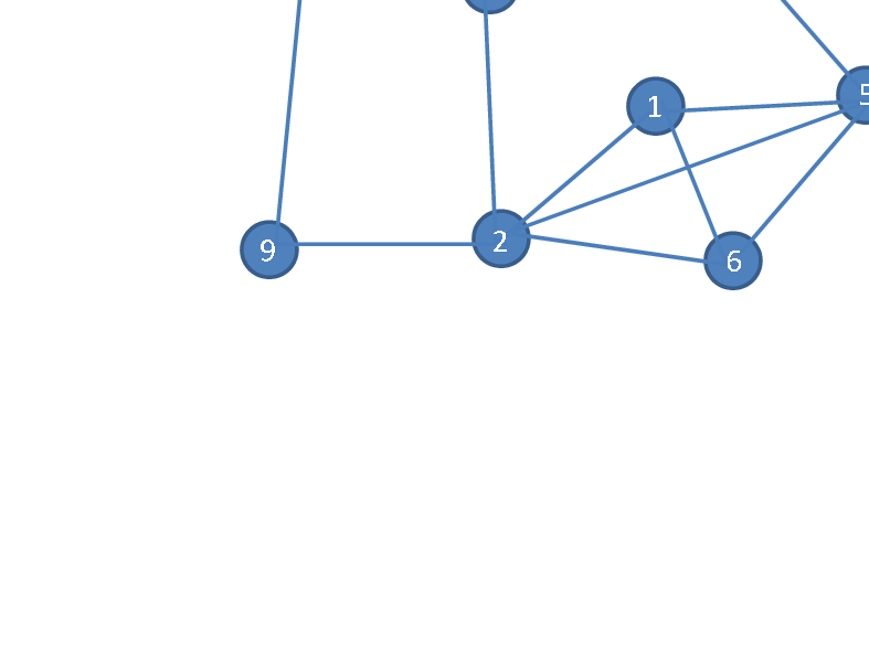
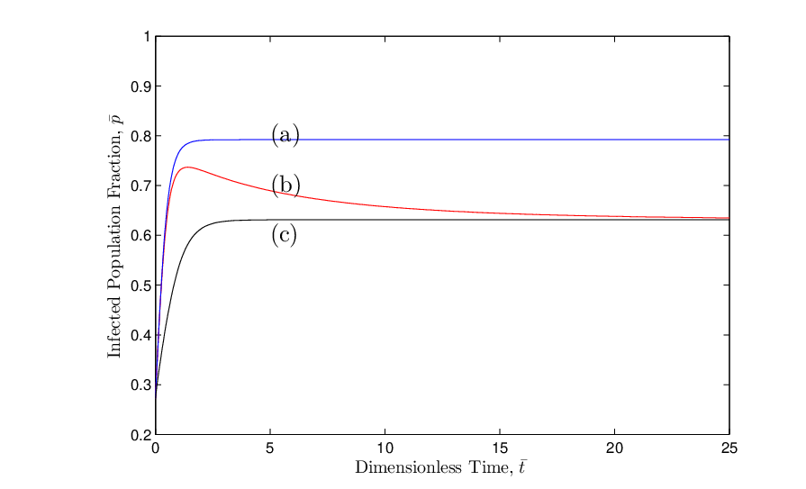
Consider a contact graph as represented in Fig. 2. For this network, the spectral radius is found to be $\rho(A)=3.1385$ . The alerting rate is arbitrarily selected as $\kappa=0.1$ . The infection rate of an alert individual $\beta_{a}$ is chosen $\beta_{a}=0.1$ . For the simulation purpose, nodes $1$ , $5$ , and $10$ are initially in the infected state. Other nodes are initialized in the susceptible state. In each simulation, the total infection fraction $\bar{p}(t)=\frac{1}{N}\sum_{i=1}^{N}p_{i}(t)$ is computed. In Fig. 3, three trajectories are plotted. The trajectory (a) corresponds to the N-intertwined SIS model, with $\beta_{0}=2$ . Trajectory (b) is the solution of the SAIS model (13) and (14) developed in Section III. Trajectory (c) is the solution of the SIS model but with the reduced infection rate $\beta_{eq}$ defined in (32). As is expected from Theorem 1, the infected fraction in the SAIS model is always less than that of the SIS model. In addition, as proved in Theorem 4, the steady state infection fraction in the SAIS in equal to that of the SIS model with the reduced infection rate $\beta_{eq}$ .

Example 2

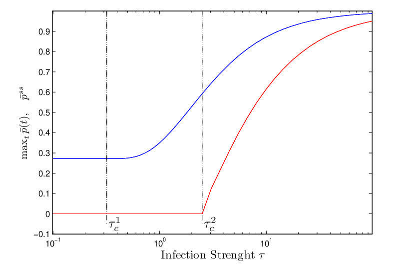
In Fig. 3, it can be observed that in the SAIS model the infection spreads similar to the SIS model at the first stage. Then, the size of the epidemics is reduced due to increased alertness in the network. In this example, for the same network in the previous example, the steady state value of the infected fraction and the maximum value of the infected fraction are presented as a function of the infection strength $\tau=\beta_{0}/\delta$ . The simulation parameters are chosen as $\kappa=1,$ $\beta_{a}=0.1$ . Note that $\beta_{a}/\delta=0.1<1/\rho(A)=0.3186$ . Therefore, as discussed in Remark 6, there exists two distinct thresholds $\tau_{c}^{1}$ and $\tau_{c}^{2}$ presented in (45) and (49), respectively. Simulation results for this example are shown in Fig. 4.

Example 3

As is observed in Fig. 4, the steady state values of the infected fraction $\bar{p}$ is zero before the second epidemic threshold $\tau_{c}^{2}$ . In addition, the maximum of the infected fraction is equal to the initial infected fraction before $\tau_{c}^{1}$ . The reason for this observation is that before the first threshold $\tau_{c}^{1}$ , the epidemics dies out exponentially; as stated in Theorem 2. Between the two thresholds, $\max_{t}\bar{p}(t)$ is greater than $\bar{p}(0)$ but steady state value $\bar{p}^{ss}=0$ . In other words, in this region the epidemic spreads at the first stage but then is completely controlled as a result of increased alertness. After the second threshold, $\bar{p}^{ss}<\max_{t}\bar{p}(t)$ , i.e., alertness reduced the size of the epidemic.

Example 4

Consider an epidemic network where the contact graph is an Erdos-Reyni random graph with $N=320$ nodes and connection probability $p=0.2$ . The initial infected population is $\%2$ of the whole population. The simulation parameters are $\beta_{0}=0.03$ , $\kappa=0.05$ . Three trajectories are presented in Fig. 5. The trajectory (a) is for the SIS model, i.e., no alertness exists. Trajectory (b) is for $\beta_{a}=0.02$ . In this case, the epidemic size is reduced in the steady state. Trajectory (c) corresponds to $\beta_{a}=0.01$ , for which the epidemic dies out asymptotically. For the sake of evaluating the model development in Section III, a Monte-Carlo simulation is also provided for each trajectory and shown in the figure in blue. As can be seen, there is a reasonable agreement between the proposed model (13) and (14) and the Markov process (9).

VI Acknowledgement

This research is supported by National Agricultural Biosecurity Center at Kansas State University. Authors would also like to thank Dr. Fahmida N. Chowdhury for her constructive feedbacks on this manuscript.

VII Conclusion

In this paper, we add a new compartment to the classic SIS model to account for human response to epidemic spread. Each individual can be infected, susceptible, or alert. Susceptible individuals can become alert with an alerting rate if infected individuals exist in their neighborhood. An individual in the alert state is less probable to become infected than an individual in the susceptible state; due to a newly adopted cautious behavior. The problem is formulated as a continuous time Markov process on a general static graph and then modeled into a set of ordinary differential equations using mean field approximation method and the corresponding Kolmogorov forward equations. The model is then studied using results from algebraic graph theory and center manifold theorem. We analytically show that our model exhibits two distinct thresholds in the dynamics of epidemic spread. Below the first threshold, infection dies out exponentially. Beyond the second threshold, infection persists in the steady state. Between the two thresholds, the infection spreads at the first stage but then dies out asymptotically as the result of increased alertness in the network. Finally, simulations are provided to support our findings. Our results suggest that alertness can be considered as a strategy of controlling the epidemics which propose multiple potential areas of applications, from infectious diseases mitigations to malware impact reduction. Generalizing the current results to time-varying weighted topologies is a promising extension.

References

[1] N. Ferguson, “Capturing human behaviour,” Nature, vol. 446, no. 7137, p. 733, 2007.
[2] S. Funk, M. Salath, and V. A. A. Jansen, “Modelling the influence of human behaviour on the spread of infectious diseases: a review,” Journal of The Royal Society Interface, vol. 7, pp. 1247–1256, 2010.
[3] G. Theodorakopoulos, J.-Y. L. Boudec, and J. S. Baras, “Selfish response to epidemic propagation,” in American Control Conference, 2011, to apear.
[4] S. Kitchovitch and P. Lio, “Risk perception and disease spread on social networks,” Procedia Computer Science, vol. 1, no. 1, pp. 2339–2348, 2010.
[5] X. Zeng and M. Wagner, “Modeling the effects of epidemics on routinely collected data,” Journal of the American Medical Informatics Association, vol. 9, no. Suppl 6, p. S17, 2002.
[6] C. Bauch and D. Earn, “Vaccination and the theory of games,” Proceedings of the National Academy of Sciences of the United States of America, vol. 101, no. 36, pp. 13 391–4, 2004.
[7] F. Chen, “A susceptible-infected epidemic model with voluntary vaccinations,” Journal of mathematical biology, vol. 53, no. 2, pp. 253–272, 2006.
[8] S. Funk, E. Gilad, C. Watkins, and V. Jansen, “The spread of awareness and its impact on epidemic outbreaks,” Proceedings of the National Academy of Sciences, vol. 106, no. 16, pp. 6872–6877, 2009.
[9] S. Funk, E. Gilad, and V. Jansen, “Endemic disease, awareness, and local behavioural response,” Journal of Theoretical Biology, vol. 264, no. 2, pp. 501–509, 2010.
[10] I. Kiss, J. Cassell, M. Recker, and P. Simon, “The impact of information transmission on epidemic outbreaks,” Mathematical biosciences, vol. 225, no. 1, pp. 1–10, 2010.
[11] S. Tracht, S. Del Valle, J. Hyman, and D. Carter, “Mathematical modeling of the effectiveness of facemasks in reducing the spread of novel influenza a (h1n1),” PloS one, vol. 5, no. 2, p. e9018, 2010.
[12] A. McKendrick, “Applications of mathematics to medical problems,” Proceedings of the Edinburgh Mathematical Society, vol. 44, pp. 98–130, 1925.
[13] N. Bailey, The mathematical theory of infectious diseases and its applications. London, 1975.
[14] Y. Moreno, R. Pastor-Satorras, and A. Vespignani, “Epidemic outbreaks in complex heterogeneous networks,” The European Physical Journal B - Condensed Matter and Complex Systems, vol. 26, pp. 521–529, 2002.
[15] R. Pastor-Satorras and A. Vespignani, “Epidemic dynamics and endemic states in complex networks,” Phys. Rev. E, vol. 63, no. 6, p. 066117, May 2001.
[16] Y. Wang, D. Chakrabarti, C. Wang, and C. Faloutsos, “Epidemic spreading in real networks: An eigenvalue viewpoint,” Proc. 22nd Int. Symp. Reliable Distributed Systems (SRDS03), p. 2534, 2003.
[17] D. Chakrabarti, Y. Wang, C. Wang, J. Leskovec, and C. Faloutsos, “Epidemic thresholds in real networks,” ACM Transactions on Information and System Security (TISSEC), vol. 10, no. 4, pp. 1–26, 2008.
[18] A. Ganesh, L. Massoulie, and D. Towsley, “The effect of network topology on the spread of epidemics,” in INFOCOM 2005. 24th Annual Joint Conference of the IEEE Computer and Communications Societies. Proceedings IEEE, vol. 2, 2005, pp. 1455–1466, 1/rho.
[19] P. Van Mieghem, J. Omic, and R. Kooij, “Virus spread in networks,” Networking, IEEE/ACM Transactions on, vol. 17, no. 1, pp. 1–14, 2009.
[20] V. Preciado and A. Jadbabaie, “Spectral analysis of virus spreading in random geometric networks,” in Decision and Control, Proc. of the 48th IEEE Conference on. IEEE, 2010, pp. 4802–4807.
[21] ——, “Moment-based analysis of spreading processes from network structural information,” Arxiv preprint arXiv:1011.4324, 2010.
[22] P. Poletti, B. Caprile, M. Ajelli, A. Pugliese, and S. Merler, “Spontaneous behavioural changes in response to epidemics,” Journal of Theoretical Biology, vol. 260, no. 1, pp. 31–40, 2009.
[23] R. Diestel, “Graph theory, volume 173 of graduate texts in mathematics,” Springer, Heidelberg, vol. 91, p. 92, 2005.
[24] J. Carr, Applications of Center Manifold Theory. Springer-Verlag, 1981.
[25] H. Khalil and J. Grizzle, Nonlinear systems. Prentice hall Englewood Cliffs, NJ, 2002, vol. 3.
[26] D. Stroock, An introduction to Markov processes. Springer Verlag, 2005.
[27] P. Van Mieghem, Performance analysis of communications networks and systems. Cambridge Univ Pr, 2006.