Constraints on Enhanced Dark Matter Annihilation from IceCube Results
Abstract
Excesses on positron and electron fluxes measured by ATIC, and the PAMELA and Fermi–LAT telescopes can be explained by dark matter annihilation in our Galaxy. However, this requires large boosts on the dark matter annihilation rate. There are many possible enhancement mechanisms, such as the Sommerfeld effect or the existence of dark matter clumps in our halo. If enhancements on the dark matter annihilation cross section are taking place, the dark matter annihilation in the core of the Earth should also be enhanced. Here we use recent results from the IceCube 40–string configuration to probe generic enhancement scenarios. We present results as a function of the dark matter–proton interaction cross section, weighted by the branching fraction into neutrinos, , as a function of a generic boost factor, , which parametrizes the expected enhancement of the annihilation rate. We find that dark matter models which require annihilation enhancements of or more and that annihilate significantly into neutrinos are excluded as the explanation for these excesses. We also determine the boost range that can be probed by the full IceCube telescope.
Keywords:
Dark matter, Sommerfeld enhancement, Neutrinos, Neutrino Telescopespacs
95.35.+d, 95.30.Cq, 11.30.PbI Introduction
Several recent observations in our galaxy have found an excess on the electron and/or positron fluxes [1, 2, 3]. However the origin of these events is yet not clear. If they are produced accordingly to standard physics, pulsars [4] might be their sources as well as they could be secondary particles created by shock accelerated hadrons [5]. Another exciting possibility is that they can be a signature of new physics. It was shown that dark matter annihilation in the galaxy can describe the data [6]. However most of these models require an enhancement on its annihilation rate. An enhancement mechanism can be found from a variety of possible phenomena, such as the Sommerfeld effect, the existence of dark matter substructures in the galactic halo, or a combination of both [7, 8].
Constraints on a boost factor on the dark matter annihilation rate have been recently derived from the Fermi–LAT diffuse gamma–ray measurement [9] and from their analysis of Milky Way satellite galaxies [28]. An independent and neat analysis has been performed by the authors of Ref [10], using the fact that dark matter annihilations at recombination time, redshift 1000, would have injected secondary particles that would have affected the recombination processes. The measured power spectrum of the cosmic microwave background (CMB) can thus be used to set limits on the strength of the dark matter self–annihilation cross section. The IceCube collaboration has also performed an analysis searching for dark matter annihilations in the galactic halo by searching from an excess diffuse neutrino flux over the expected atmospheric flux [11]. The results can also be used to set limits on a boost in the annihilation cross section.
These methods show some degree of complementarity since each one provides better sensitivity to a different range of the mass of the dark matter particles or to different annihilation channels. They also rest on different assumptions and approximations. Fermi and the CMB method are competitive in the low mass range (dark matter massed 1 TeV), while IceCube reaches 10 TeV, and can also probe annihilation directly into neutrinos. There is some halo-model dependency when setting limits on the annihilation cross section from the observations of satellite galaxies: the expected signal depends on the degree of cuspiness of the assumed halo. On the other hand, the CMB analysis does not depend on the shape of dark matter haloes, since there are no gravitationally bound structures at the redshift considered, but it depends on assumptions about the fraction of the energy released by the annihilating dark matter particles and how it is absorbed by the surrounding medium.
In this paper we follow the alternative approach proposed in Ref. [12]. The authors argue that an enhancement of the dark matter annihilation rate should also boost the neutrino flux from dark matter annihilations in the center of the Earth. A thermal annihilation cross section implies that dark matter capture and annihilation has not yet reached equilibrium in the Earth. However it is not necessary that the annihilation cross section has to remain the same as during the freeze–out period. If the annihilation rate is somehow enhanced in the post freeze–out period, the equilibrium might already have been achieved. As it will be shown in the next Section, the annihilation rate reaches its maximum at the equilibrium, and then depends only in the capture rate. A boost in the annihilation rate increases the flux of annihilation products until it reaches its maximum. In this case the neutrino flux from the center of the Earth will be large enough to be detected by telescopes such as IceCube. In short, if the dark matter annihilation rate is enhanced, the timescale for equilibrium diminishes and the flux of annihilation products is expected to be much larger than the one away from equilibrium.
We use the recently published IceCube results on a search for a diffuse flux of muon neutrinos [13] to set limits on a boost factor in the dark matter annihilation cross section. IceCube has measured neutrinos coming from near or below the horizon in the energy range 332 GeV and 84 TeV using data taken with the 40–string detector configuration (IceCube–40). The analysis includes all events coming from near or below the horizon, and the result is compatible with the expected atmospheric neutrino flux (see also Ref. [14]). It is also generic enough to allow comparison with our prediction of the flux of muon neutrinos produced in dark matter annihilations in the center of the Earth. We determine this flux by simulating the annihilation of WIMP–type particles in the center of the Earth and propagating the neutrinos to the detector. A significant neutrino flux from dark matter annihilation should be seen above the expected atmospheric neutrino flux. If not, limits can be set on the model used to determine the dark matter signal. Our analysis shows that models which require very large boosts on the dark matter annihilation rate in order to explain the excess seen in the galactic positron and electron flux, and have an annihilation channel into neutrinos, are ruled out.
In the next Section we describe dark matter capture and annihilation in the Earth. In Sections III and IV we describe the signal simulation and calculate the expected number of events in the IceCube–40 detector. We then compare our results with the IceCube–40 published results, showing the boost factor range that is excluded. Finally, in Section V we estimate the sensitivity region for the full 86–string detector.
II Dark matter annihilation in the Earth
Dark matter interactions in the Earth will be dominated by spin–independent elastic scattering, since the most abundant isotopes of the Earth core and mantle are spin 0 nuclei. The time evolution of the number of dark matter particles will result from a balance between the capture () and annihilation rate ():
| (1) |
| (2) |
here is the spin–independent dark matter cross section off protons, and are the dark matter velocity and density in the halo and is the dark matter particle mass. In deriving the above equation it has been assumed that for masses mχ much larger than the nucleus mass, the dark matter interaction cross section off a proton is the same as off a neutron. In this case, the spin–independent cross section off a nucleus with mass number A is given by , where is the proton mass.
The annihilation rate depends both on the relative velocity scaled cross section as well as on the dark matter distribution in the Earth [16]. The latter can be given in terms of the parameter , where , and cm3 represents the dark matter effective volume in the core of the Earth, assuming an isothermal distribution [17, 15].
The solution to the dark matter time evolution in the Earth (Equation 1) is then,
| (3) |
where is the age of the solar system and is the timescale for equilibrium between capture and annihilation. An enhancement on the annihilation rate will only be effective if it can accelerate equilibrium within the Earth. When the equilibrium stage is reached, the annihilation is maximum and depends entirely on the capture rate (). Thermal relic dark matter candidates typically have cm3s-1, which makes s-1 and for these values the Earth is today far from equilibrium.
In our analysis we consider scenarios where the annihilation cross section is enhanced by boosting the thermal relic annihilation rate by a generic factor which affects the non–equilibrium rate through . Such parametrization, though adequate to probe enhancements due to Sommerfeld effect or to new interaction mechanisms, cannot probe enhancements due to a possible dark matter halo substructure. In this latter case, a standard annihilation cross section could well account for any possible signal, which would be just due to the increased local dark matter density, and not due to any new feature of the annihilation process itself.
III Neutrino Production
The escape velocity at the Earth core is km/s and dark matter moves very slowly inside the Earth. The annihilation products will therefore be monochromatic, and produced with the same energy as the dark matter mass. Here we consider the annihilation into a muon neutrino pair (which we call primary neutrinos). “Secondary” neutrinos are also produced in the decay of other primary annihilation particles, such as ’s, t’s, W’s and b’s. Since the explanation of the observed leptonic excess in terms of dark matter has also to account for the fact that no antiproton excess was found by PAMELA [18], annihilation into leptons is preferred when compared to hadrons. Secondary neutrinos from annihilation into charged lepton states, specifically on were analyzed in Ref. [12]. The energies of these secondary neutrinos will be spread at relatively low values ( GeV) compared to the primary neutrino flux, and detection in neutrino telescopes is then disfavored (unreasonably large boost factors would be needed to bring such flux over the atmospheric neutrino background to a detectable level). We will therefore not take into account the secondary neutrino flux in our calculations, and concentrate in the easily detectable monochromatic flux from direct annihilations.
The primary neutrino flux, produced from dark matter annihilations in the Earth’s center is given by:
| (4) |
where is the annihilation branching ratio into , is the radius of the Earth, and is the energy distribution of the neutrinos produced in the annihilations. We show our results for two generic cases, GeV and GeV, which are representative of the models which fit the observed positron and electron excess, and later on for GeV when comparing our results to others. Since at these energies neutrinos practically do not lose energy in their way from the center of the Earth to the detector, the term will then be a delta function at the dark matter masses considered.
IV Constraints on the annihilation boost factor from IceCube–40
In order to predict the muon flux from dark matter annihilation in the Earth at the IceCube detector in the South Pole, we use the publicly available WimpSim code [19]. We simulate a monochromatic muon neutrino beam at the center of the Earth, with energy equal to the dark matter mass, by selecting the muon neutrino channel. WimpSim simulates the propagation of these neutrinos, including energy losses and charged and neutral current interactions as well as oscillations through the Earth. The muon neutrino flux at the detector is given as an output. Although we have chosen to simulate the flux specifically for the location of the IceCube detector, the detector site is not relevant in this case, and the results and sensitivities presented in the next sections can easily be interpreted for any neutrino telescope of similar size.
The number of muons from dark matter annihilation from a given angular region and during an exposure in IceCube–40, is then:
| (5) |
We proceed then by convoluting the muon neutrino flux with the IceCube–40 effective area published in Ref. [13]. The effective area accounts for the detector efficiency including the neutrino–nucleon interaction probability, the muon energy loss from its production point to the detector, and the detector trigger and analysis efficiency. As the neutrino beam is monochromatic, we use the corresponding value of for each dark matter mass considered. The muon–neutrino angular distribution is the main parameter for background reduction in our analysis. Figure 1 shows the angular distribution from neutrinos from dark matter annihilation in the center of the Earth. It is collimated in a angle of less than approximately around the vertical direction, . This figure also shows the smearing effect due to the angular resolution of the detector, taken here conservatively to be 2∘ for up–going vertical events. We use therefore the effective area for the zenith range from Ref. [13]. Even though such angular range is much wider than that from the expected signal, the effective area does not vary considerably with zenith angle below about 10 TeV, where Earth absorption effects start to be important.
For our analysis, we choose an angular window from the vertical direction that contains 90% of the expected signal (() for 500(1000) GeV dark matter respectively, where the angular experimental resolution has been taken into account), and use the calculated number of events with Eq. 5 as signal. We have not used any energy information in this analysis, just using the total number of events predicted and detected to derive our exclusion regions. We will however present a study on the effect of the detector energy resolution in the sensitivity study for the complete IceCube detector in the next section. Figure 2 shows the predicted number of in IceCube–40, with days as a function of the dark matter nucleon cross section scaled by the branching ratio for different boosts factors. As can be seen, larger enhancements on the annihilation rate result in a shorter time for equilibrium among capture and annihilation.
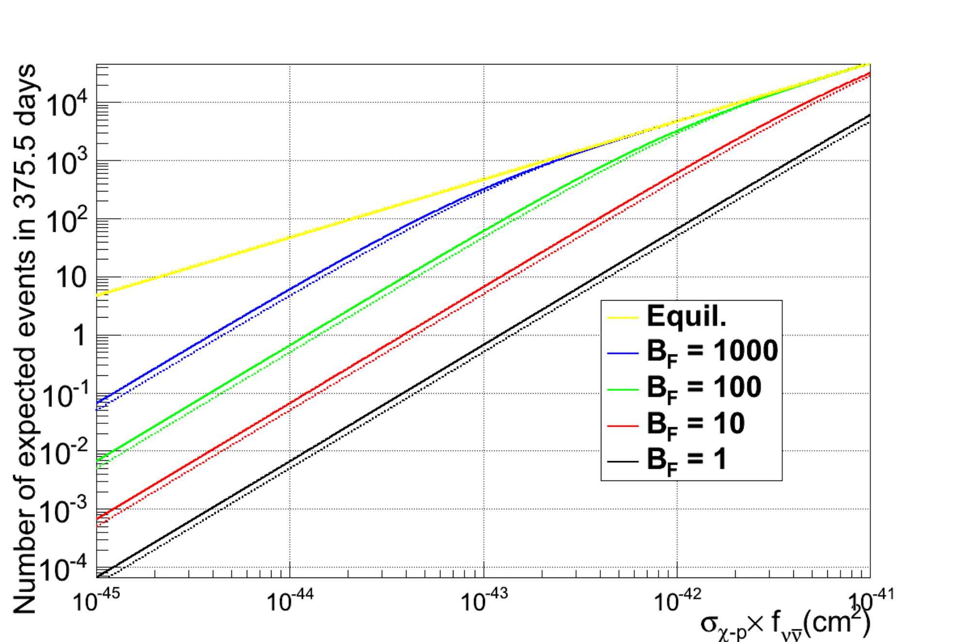
In order to study the model rejection power of our analysis in a quantitative way, we determine the statistical significance of the predicted dark matter signal, , as a function of boost factor, where is the number of signal events predicted in the given angular cone. As background, , we use the measured number of events in IceCube–40 in the same angular regions.
Two recent IceCube publications, a measurement of the atmospheric neutrino flux [14] and a search for a diffuse flux of cosmic origin [13], give results that are consistent with the expected atmospheric neutrino flux. We use the publicly available data from the diffuse analysis which is available at Ref. [20]. This analysis selects events coming from near or below the horizon and their background is composed by atmospheric muons arriving from above the detector and misreconstructed as an event coming from below. The rejection of these events is described in Ref. [13] and the background contamination in the data sample is estimated to be less than 1%. The final data sample contains 13K events and it is given as a function of the zenith angle. This allows us to select events which come in the same direction as expected signal dark matter annihilations. The data is then reduced to 14 (9) events when considering the angular regions expected for 500 (1000) GeV dark matter neutrinos. We compare this number to the predicted number of events from our signal choices and for different boost factors.

The result is presented in Fig. 3, which shows the boost factor versus scaled by the branching ratio region which was probed in this analysis. The plot to the left is for 500 GeV dark matter and the one to the right is for 1 TeV. The light green full line shows a exclusion and above this line the exclusion is more strict according to the color coded bar on the right side. This bar indicates the level of statistical significance. The best limit on comes from the Xenon100 collaboration [23]. At 90% CL 500 GeV dark matter models are constrained above cm2 and 1 TeV dark matter above cm2. We draw this limit on Fig. 3 just as a reference, since direct detection results do not depend on neither on any boost factor. For such limit, boost factors above 215 and 58 respectively are excluded at a level. This exclusion requires, however, that , ie., annihilation exclusively into neutrinos, which may be difficult to justify phenomenologically. But it should be noted that the excluded region in Fig. 3 does not require necessarily a 100% annihilation into neutrinos. One can lower the branching factor by increasing the required boost factor limit. As one moves down along the green 5 limit line, larger boost factors are disfavored, as the quantity becomes lower. Lower values of can be achieved either by models with relatively high cross sections but a lower branching ratio to neutrinos, or by lower cross sections but a higher annihilation probability to neutrinos. In either case, the expected signal in IceCube would decrease and a higher boost factor would be needed to bring it to the current sensitivity of the detector. Higher boost factors to the right of the green line would then be disfavored at a higher significance.
The degeneracy of the product can be broken when considering specific dark matter models with known branching ratio to neutrinos and cross section with protons. Fig. 3 can then be used to determine the minimum boost factor which is disfavored at a 5 level.
V Prediction for full IceCube detector
The full IceCube detector with 86 strings (IceCube–86) is now completed and taking data since May 2011. In order to estimate the full detector sensitivity, we can use the fact that the atmospheric neutrino flux measured by IceCube–40 [13, 14] is consistent with model expectations as, for example, the one proposed by Ref. [21]. We will also go one step further than in the calculations of the previous Section, and assume that IceCube will be able to estimate the neutrino energy with a given resolution . We assume three benchmark energy resolutions, and which go from the very optimistic to the more conservative situation in a neutrino telescope. The 40–string configuration has its energy resolution between 50% and 80%. We assume here that the complete detector can reach a better resolution in any case. We note that energy estimation in neutrino telescopes is a difficult task since muon tracks above a few hunderd GeV will cross the detector volume, and the neutrino energy can only be estimated through model–dependent deconvolution methods.
An effective area at trigger level for the complete IceCube–86 detector has been published in Ref. [25]. However the effective area at final analysis level can differ significantly from trigger level, since data quality cuts are applied to the data sample to reduce background, but also inevitably reducing signal efficiency. In practice, one can just rescale the IceCube–40 effective area by 2.15 (which factors 40 to 86 strings), since at the energies considered in our analysis, and for vertical events, each string is practically an independent detector and therefore, in a first approximation, the effective area scales proportionally to just the number of strings. We expect, though, dedicated analysis with IceCube–86 to be more efficient at lower energies than the IceCube–40 analysis we have used in the previous Section and, since we will be integrating A in a range of energies, we need to be careful with the behavior of the effective area with energy. We have therefore normalized the IceCube–86 effective area from Ref. [25] with the rescaled IceCube–40 area at 10 TeV, where the IceCube–40 analysis is optimal. The shape of the IceCube–86 effective area at lower energies takes automatically into account the improved capabilities of the full detector at energies below 1 TeV.
We have then all the ingredients we need to estimate the sensitivity of the IceCube–86 detector. We calculate the number of atmospheric neutrino events from within a vertical cone of 4.1∘ and 3.7∘ aperture by convoluting the detector effective area with the parametrization of the atmospheric neutrino flux taken from Ref. [21]. Instead of choosing a delta function for the spectrum as in the previous case, we introduce a smearing in the energy according to the assumed energy resolution. In practice, this translates into that we perform the A integral between m and m. We assume that the measurement of IceCube will be compatible with the calculated number of background events and calculate the sensitivity to an excess neutrino flux from the center of the Earth under this assumption. The result of this exercise is shown in Fig. 3. The dashed black (red,blue) lines in both plots represent sensitivity that can be achieved in one year live time of IceCube–86 ( d) assuming a 50 (30,10)% energy resolution.
VI Conclusions
If dark matter annihilation in our galaxy is responsible for the excesses seen by ATIC [1], PAMELA [2] and Fermi–LAT [3], an enhancement on the dark matter annihilation rate in the Earth should also be foreseen. This enhancement might bring the equilibrium among the dark matter capture and annihilation rates to occur much earlier than the timescale expected from a purely thermal annihilation rate. In this case the neutrino flux from dark matter captured in the Earth can be quite large. We present results as a function of the dark matter–proton interaction cross section, weighted by the branching fraction into neutrinos, , as a function of a generic boost factor, , which parametrizes the expected enhancement of the annihilation rate. In this sense, it is important to note that our results do not depend on the details of the mechanism which enhances the annihilation cross section. We have used two benchmark models, a 500 GeV and 1 TeV generic WIMP annihilating in the center of the Earth to scan the (, ) parameter space and set constrains on this 2-dimensional space using current IceCube results. Our calculations assume that the dark matter velocity distribution is Gaussian as well as that dark matter collected in the Earth’s core follows an isothermal distribution.
In order to explain the positron and electron excesses that are seen, models also have to cope with the fact that the antiproton spectrum measured by PAMELA [18] is in full agreement with the expectation from secondary production of antiprotons from propagation of cosmic rays in the galaxy. This rules out as an explanation of the excess many dark matter models with preferred annihilation into heavy products, producing many antiprotons. Therefore leptophilic models, which propose dark matter annihilation exclusively into leptons, are favored as an explanation to the excesses found. We have shown that, when 500 (1000) GeV dark matter annihilates into a large fraction of neutrinos, annihilation boost factors of the and above are already constrained by our analysis at a 5 level, or higher, depending on the interaction cross section assumed. Thus, leptophilic models [26] which favor primary neutrino production are constrained by our results.
In order to compare this analysis to others, we show in Figure 4 limits on as a function of from Fermi [28], CMB [10] and IceCube [29]. Our bounds as a function of , can be determined from equation 3. It can also easily be visualized in Figure 3, where a significance is shown as the edge of the shaded area: the limit on the annihilation cross section is determined from each boost factor value on this curve. In Figure 4 these are shown for two choices of , cm2 (blue stars) and cm2 (blue solid squares), which are below the current Xenon limit [23].
Our results and IceCube’s, are the only ones to probe annihilation into neutrinos. Other limits coming from searches with gammas from satellite galaxies by Fermi [28] or from the analysis based on the CMB [10] imprint at high redshifts, are complementary, since not only they probe different annihilation channels, but also rest on different underlying assumptions.
We also investigated the reach of the completed IceCube 86-string detector, and we present results of its sensitivity in the (, ) parameter space. We have estimated how using neutrino energy information could improve the analysis, and in Fig. 3 we show the expected sensitivity for three different assumptions of the detector energy resolution.
Acknowledgements.
We thank P. Fox and P. Gouffon for fruitful discussions. IA was partially funded by the Brazilian National Counsel for Scientific Research (CNPq), and L.J.B.S. was partially funded by the State of São Paulo Research Foundation (FAPESP) and by CNPq.References
- [1] J. Chang et al,, Nature 456 (2008) 362.
- [2] O. Adriani et al,, PAMELA Collaboration, [arXiv:1103.2880]; Astropart. Phys. 34, 1-11 (2010). [arXiv:1001.3522]; O. Adriani et al,, PAMELA Collaboration, Phys. Rev. Lett. 102, 051101 (2009). [arXiv:0810.4994].
- [3] A. A. Abdo et al,, Fermi–LAT Collaboration, Phys. Rev. Lett. 102, 1811101 (2009).
- [4] S. Profumo, Central Eur. J. Phys. 10, 1 (2011) [arXiv:0812.4457 [astro-ph]].
- [5] P. Blasi, Phys. Rev. Lett. 103, 051104 (2009). [arXiv:0903.2794].
- [6] M. Cirelli and A. Strumia, PoS IDM2008, 089 (2008). [arXiv:0808.3867]; I. Cholis, L. Goodenough, D. Hooper, M. Simet and N. Weiner, Phys. Rev. D80, 123511 (2009). [arXiv:0809.1683]; I. Cholis, L. Goodenough, D. Hooper, M. Simet and N. Weiner, Phys. Rev. D80, 123511 (2009). [arXiv:0809.1683]. D. P. Finkbeiner, L. Goodenough, T. R. Slatyer, M. Vogelsberger and N. Weiner, JCAP 1105, 002 (2011). [arXiv:1011.3082].
- [7] I. Cholis and L. Goodenough, JCAP 1009, 010 (2010).
- [8] M. Lattanzi and J. Silk, Phys. Rev. D79, 083523 (2009).
- [9] A. A. Abdo et al,, Fermi–LAT Collaboration, JCAP 1004, 014 (2010), [arXiv:1002.4415];
- [10] S. Galli, F. Iocco, G. Bertone and A. Melchiorri, Phys. Rev. D 84, 027302 (2011). [arXiv:1106.1528 [astro-ph.CO]]; G. Hütsi, J. Chluba, A. Hektor and M. Raidal, Astron. & Astrophys. 535, A26 (2011).
- [11] R. Abbasi et al, IceCube Collaboration, Phys. Rev. D84, 022004 (2011).
- [12] C. Delaunay, P. J. Fox and G. Perez, JHEP 0905, 099 (2009). [arXiv:0812.3331].
- [13] R. Abbasi et al,, IceCube Collaboration, Phys. Rev. D84, 082001 (2011). [arXiv:1104.5187].
- [14] R. Abbasi et al, IceCube Collaboration, Phys. Rev. D83, 012001 (2011). [arXiv:1010.3980].
- [15] G. Jungman, M. Kamionkowski and K. Griest, Phys. Rept. 267, 195-373 (1996). [hep-ph/9506380].
- [16] K. Griest and D. Seckel, Nucl. Phys. B283, 681 (1987).
- [17] A. Gould, Astrophys. J. 321, 571 (1987).
- [18] O. Adriani et al,, PAMELA Collaboration, Phys. Rev. Lett. 105, 121101 (2010). [arXiv:1007.0821].
- [19] M. Blennow, J. Edsjö and T. Ohlsson, JCAP 0801, 021 (2008). [arXiv:0709.3898].
- [20] http://www.icecube.wisc.edu/science/data/.
- [21] M. Honda et al, Phys. Rev. D75, 043006 (2007). [astro-ph/0611418].
- [22] G. Feldman and R. D. Cousins, Phys. Rev. D57, 3873 (1998).
- [23] E. Aprile et al,, XENON100 Collaboration, Phys. Rev. Lett. 107, 131302, (2011). [arXiv:1104.2549].
- [24] Z. Ahmed et al,, CDMS–II Collaboration, Science 327, 1619-1621 (2010). [arXiv:0912.3592].
- [25] C. Wiebusch, for the IceCube Collaboration, Procc. of the 31st ICRC, Lodz, Poland, July 2009 [arXiv:0907.2263].
- [26] P. J. Fox and E. Poppitz, Phys. Rev. D79, 083528 (2009). [arXiv:0811.0399].
- [27] R. Abbasi et al, [IceCube Collaboration], Phys. Rev. D 84, 022004 (2011) [arXiv:1101.3349 [astro-ph.HE]].
- [28] A. Ackermann et al,, Fermi–LAT Collaboration, Phys. Rev. Lett. 107, 241302 (2011).
- [29] A. Abbasi et al,, IceCube Collaboration, Phys. Rev. D84, 022004, (2011); see also [arXiv:1111.2738]