ON MODELING OF STATISTICAL PROPERTIES OF CLASSICAL 3 SPIN GLASSES
Abstract
ABSTRACT
We study statistical properties of 3 classical spin glass layer
of certain width and infinite length. The 3 spin glass is
represented as an ensemble of disordered 1 spatial spin-chains
(SSC) where interactions are random between spin-chains (nonideal
ensemble of 1 SSCs). It is proved that at the limit of Birkhoff’s
ergodic hypothesis performance 3 spin glasses can be generated by
Hamiltonian of disordered 1 SSC with random environment.
Disordered 1 SSC is defined on a regular lattice where one
randomly oriented spin is put on each node of lattice. Also it is
supposed that each spin randomly interacts with six
nearest-neighboring spins (two spins on lattice and four in the
environment). The recurrent transcendental equations are obtained on
the nodes of spin-chain lattice. These equations combined with the
Silvester conditions allow step by step construct spin-chain in the
ground state of energy where all spins are in minimal energy of
classical Hamiltonian. On the basis of these equations an original
high-performance parallel algorithm is developed for 3 spin
glasses simulation. Distributions of different parameters of
unperturbed spin glass are calculated. In particular, it is
analytically proved and by numerical calculations shown that the
distribution of spin-spin interaction constant in Heisenberg
nearest-neighboring Hamiltonian model as opposed to widely used
Gauss-Edwards-Anderson distribution satisfies Lévy alpha-stable
distribution law which does not have variance. A new formula is
proposed for construction of partition function in kind of
one-dimensional integral on energy distribution of 1 SSCs.
pacs
71.45.-d, 75.10.Hk, 75.10.Nr, 81.5Kfkeywords: Spin-glass Hamiltonian, random network, Birkhoff ergodic hypothesis, statistic distributions, parallel algorithm, numerical simulation.
I Introduction
The wide class of phenomena and structures in
physics, chemistry, material science, biology, nanoscience,
evolution, organization dynamics, hard-optimization, environmental
and social structures, human logic systems, financial mathematics,
etc. are mathematically well described in the framework of spin
glass models [1, 2, 3, 5, 6, 4, 7, 8, 9].
The considered mean-field models of spin glasses as a rule are
divided into two types. The first consists of the true random-bond
models where the coupling between interacting spins are taken to be
independent random variables [10, 11, 12].
The solution of these models is obtained by -replica trick
[10, 12] and requires invention of sophisticated
schemes of replica-symmetry breaking [12, 13]. In the
models of second type the bond-randomness is expressed in terms of
some underlining hidden site-randomness and is thus of a superficial
nature. It has been pointed out in the works
[14, 15, 16], however, this feature retains an
important physical aspect of true spin glasses, viz. they are random
with respect to the positions of magnetic impurities.
Note that all mentioned investigations as a rule conduct at
equilibrium’s conditions of medium. This fact plays a key role both
in analytical and numerical simulation by Monte Carlo
method.
Recently, as authors have shown [17] some type of dielectrics
can be studied by model of quantum 3 spin glass. In particular,
it was proved that the initial 3 quantum problem on scales of
space-time periods of an external fields can be reduced to two
conditionally separable 1 problems where one of them describes an
ensemble of disordered 1 spatial spin-chains between which are
random interactions (further will be called nonideal
ensemble).
In this paper we discuss in detail statistical properties of
classical 3 spin glass with suggestion that interactions between
spins have short-range character. We prove that nonideal ensemble
of 1 SSCs exactly describes the statistical properties of
classical 3 spin glasses in the limit of Birkhoff’s ergodic
hypothesis performance. In the work a new high performance algorithm
for simulation of this traditionally difficult calculated problem is
developed.

In section II the classical spin glass problem on 3 lattice is formulated. Equations for stationary points and corresponding Silvester conditions are obtained for definition of energy minimum on lattice nodes (local minimum of energy). The formula for computation of different parameters distributions of spin glass is defined.
In section III a theorem on reduction of 3 spin glass problem to the problem of nonideal ensemble of 1 SSCs is proved.
In section IV numerical experiments are adduced for unperturbed 1 SSCs ensemble with spin-chain’s length . In particular, distributions of energy, polarization and spin-spin interaction constants of nonideal ensemble are investigated in detail.
In section V partition function is investigated in detail in the configuration integral’s representation. A new representation is suggested for partition function in kind of one dimensional integral on energy distribution of nonideal ensemble.
In section VI the obtained theoretical and computational results are analyzed. It is very important to note that it has been proved that in the framework of the developed method it is always possible to exactly compute the ground state energy of 3 spin glasses.
II Formulation of Problem
The objects of our investigation are solid-state dielectrics, type of glass (amorphous silicon dioxide). According to the numerical simulations [7], the structure of this type compound can be well described by random network (Fig. 1a). The red and brown lattice points on this figure correspond to different atoms, while the links between them correspond to covalent bounds. As a result of charges redistribution in outer electronic shells, atoms of acquire the positive charge and atoms of correspondingly the negative charge. Thus, we can consider compounds of this type as a disordered system of similar rigid dipoles (hereinafter termed as a system of disordered spins, Fig. 1b). Let us remind that under the similar rigid dipoles are meant the dipoles for which the absolute values are equal (, where and are two arbitrary dipoles), and they don’t vary under the influence of an external field.
The Hamiltonian of 3 classical spin glass system reads:
where indices and run over all nodes of 3 lattice, correspondingly denotes the coordinates of -th spin (see Fig. 1b). For further investigation we will consider a spin glass layer of certain width and infinite length (see Fig. 2). We will consider 3 compound in the framework of nearest-neighboring Hamiltonian model. Let us note that even for this relatively simplest model numerical simulations of spin glasses are extremely hard to solve NP problems.
At first we will consider an auxiliary Heisenberg Hamiltonian of the form:
| (1) |
where the first term :
describes the disordered 1 spatial spins chain (SSC) while the second term :
correspondingly describes the random surroundings of 1 SSC (see Fig. 2). In (1) and are correspondingly random interaction constants between arbitrary and spins and between and spins, and are spins (vectors) of unit length, which are randomly orientated in O(3) space. From the general reasons it follows that with the help of (1) Hamiltonian and by way of successive constructing we can restore the Hamiltonian of 3 problem. Recall that the meaning of the construction is as follows. On the first step the central spin-chain on the -axis with its surroundings from four random spin-chains is considered (see Fig. 2). On the second step as central spin-chains are considered corresponding spin-chains from the random surroundings each of which are surrounded by new four neighboring spin-chains. Thus, repeating this cycle periodically we can construct the Hamiltonian of 3 problem. This idea will be rigorously proved below.

For further investigation of spin glass problem it is useful to write Hamiltonian (1) in spherical coordinates system:
| (2) |
Now the main problem is to find the angular configurations and spin-spin interaction constants which can make the Hamiltonian minimal on each node of lattice.
Let us consider the equations of stationary point:
| (3) |
where defines the orientation of -th spin ( are correspondingly the polar and the azimuthal angles). In addition, describes the angular configuration of spin-chain consisting of spins.
In order to satisfy the conditions of local minimum (Silvester conditions) for , it is necessary that the following inequalities are carried out:
| (5) |
where and , in addition:
Recall that designates the angular configuration of the spin in case when the condition of local minimum for is satisfied.
Thus, it is obvious that the classical 3 spin glass system (see Fig. 1b) can be considered as an nonideal ensemble of 1 SSCs (see Fig. 2) and there are random interactions between spin-chains.
Now we can construct distribution functions of different parameters of 1 SSCs nonideal ensemble. To this effect it is useful to divide the nondimensional energy axis into regions , where and is the real energy axis. The number of stable 1 SSC configurations with length in the range of energy will be denoted by while the number of all stable 1 SSC configurations - correspondingly by symbol . Accordingly, the energy distribution function can be defined by the expression:
| (6) |
where distribution function is normalized to unit:
By similar way we can construct also distribution functions for polarizations, spin-spin interaction constant, etc.
III Reduction of 3 spin glass problem to 1 SSCs ensemble problem
Modeling of 3 spin glasses is a typical NP hard problem. This type of problems are hard-to-solve even on modern supercomputers if the number of spins in the system are more or less significant. In connection with told, the significance of new mathematical approaches development is obvious and on the basis of which an effective parallel algorithms for numerical simulation of spin glasses can be elaborated.
Theorem: The classical 3 spin glass problem at the limit of isotropy and homogeneity (ergodicity) of superspins distribution (sum of spins in chain) in 3 configuration space is equivalent to the problem of disordered 1 SSCs ensemble.
It is obvious that the theorem will be proved if we can prove that
in case when the distribution of superspins in 3
configuration space is homogeneous and isotropic, the following two
propositions take place:
a) In any random environment which consists of four
arbitrary spin-chains it is always possible to find at least one
physically admissible solution for spin-chain (the direct problem), and
b) It is possible to surround an arbitrary
spin-chain from the given environment with such environment which
can make it physically admissible spin-chain solution (the reverse
problem).
The direct Problem.
Using the following notation:
| (7) |
equations system (6) can be transformed to the following form:
| (8) |
where parameters and are defined by expressions:
From the system (8) we can find the equation for the unknown variable :
| (9) |
We have transformed the equation (9) to the equation of fourth order which is exactly solved further:
| (10) |
where
Note that from the condition of nonnegativity of the value under the root we can find the following nonequality:
| (11) |
In consideration of (7), we can write following conditions:
As it follows from equations (10), if the solutions in previous two nodes and are known, then the solutions in the node can be defined only by constant . In this connection a natural question arises - are there solutions for spin-chain in arbitrarily given environment?
Let us consider Silvester conditions (5) which can be written in the form of the following inequalities:
| (12) |
where constants and are defined by expressions:
So, the problem leads to the answer of the following question - are inequality (11) and (12) compatible or not. Taking into account solutions (10) it is easy to prove that conditions (12) are automatically compatible at large absolute values of . On the other hand, there is no any contradiction with condition (11).

Thus the direct problem or the proposition a) is
proved.
Now our aim is to prove the reverse problem or the proposition
b) which consists of the following. We choose a
spin-chain from the environment (see Fig. 2), for example
. In this spin-chain all angular
configurations of spins are
known but the constants that define spin-spin interactions in
spin-chain and interactions between spin-chain and its environment
still are not defined. We will prove that it is always possible to
surround each spin-chain by such environment that the selected
spin-chain will be the correct solution from the main physical laws
point of view (see conditions (4)-(5)). In the
considered case spin-chain is surrounded
by four neighbors, one of which is fully
determined while three spin-chains and
should be still specified (see Fig. 3). Recall that
the mark ”” designates a new environment with three
spin-chains. However, for simplicity we will omit or more clearly
make change them in the subsequent calculations
. The proof of
the proposition should be conducted as follows. We will suppose
that the constants of spin-spin interactions in considered chain and
corresponding parameters of two spin-chains of environment are
known. We will show that by special choosing of parameters of the
third spin-chain it is possible to ensure the condition of
local minimum energy is satisfied in the considered spin-chain.
Let us define the following denotations for constants:
| (13) |
Using (13) we can transform equations (4) to the following form:
which are equivalent to the following relations:
| (14) |
After excluding from (14) we find the following equation:
| (15) |
Having made the following designation:
we can transform equation (15) to the following form:
| (16) |
Now substituting:
| (17) |
in (16) we find the equation:
| (18) |
From (18) the following square equation can be found :
| (19) |
where the following designations are made:
Discriminant of the square equation (19) has the form:
| (20) |
which on some set of can be positive, i.e. -th spin in spin-chain will satisfy the local minimum conditions.
Let us define:
| (21) |
Substituting (21) in (16) we will find that:
After squaring we will have the following equation:
| (22) |
where the following designations are made:
The discriminant of the square equation (22) has the form:
| (23) |
Obviously there are some set of constants on which . However, it is more important to find the region of the interaction constant values for which both determinants and are positive.
In particular as the analysis of the following condition shows:
| (24) |
discriminant is always nonnegative. From the other side:
| (25) |
which will assure that discriminant is always nonnegative. A simple analysis of conditions (24) and (25) shows that they are compatible. In other words the set of constants which satisfies the energy local minimum condition is not empty and therefore the proposition b) is proved.
So, we have proved the validity of a) and b) propositions. It is obvious that at the simulation of 1 SSC problem we can by this way fill up 3 space by 1 SSC which is equivalent to obtaining 3 spin glass. In case when the number of 1 SSCs is so much that the directions of spins in 3 space are distributed isotropically and homogeneous, the statistical properties of both problems (3 spin glass and 1 SSCs nonideal ensemble) will be obviously identic.
The theorem is proved.
IV Results of Parallel Simulations


One important consequence of the theorem is that for the numerical simulation of the problem we can use the algorithm for solving the direct problem. Obviously, a large number of independent computations of 1 SSC which can be carried out in parallel and in statistical sense make it equivalent to the problem of 3 spin-glass. This approach considerably reduces the amount of needed computations and helps us effortlessly simulate statistical parameters of 3 spin glasses of large size.
The strategy of simulation consists of the following steps (see Fig. 4). At first, the angular configurations of four spin-chains are randomly generated which form random environment of the spin-chain which we plan to construct later. On a following step a set of random constants are generated, which characterizes the interactions between the random environment and the spin-chain. The interaction constants are generated by Log-normal distribution. The angular configurations of the random environment are generated the same way as it is described in [18]. Now when the environment and its influence on disordered 1 SSC are defined, we can go over to the computation of spin-chain which must satisfy the condition of local energy minimum. Note that the scheme of further computation of nonideal ensemble of 1 SSCs (see Fig. 2) is identical to the scheme of the computation of an ideal ensemble of disordered 1 SSCs (see [18]). Note that all calculations of 1 SSCs nonideal ensemble are done for spin-chains with length which require huge computational resources.
As the simulations show, for the ensemble which consists of spin-chains, the dimensional effects practically disappear (see Figs. 5a, 5b and 6) and the energy distribution has one global maximum and is precisely approximated by Gaussian distribution (see Fig. 5a).

Mean values of polarizations on coordinates are not very small, especially when it comes to coordinate (thickness of spin glass layer): and correspondingly the average energy of SSC is equal to , where , , and is the distribution function. As our numerical investigations have shown on the example of systems where thickness of spin glass layer is not so large , for a full self-averaging of superspin it is necessary to make simulations. In other words, the system can be fully ergodic in considered case if we continue the numerical simulations of the spin-chains up to times.
It is analytically proved and also the parallel simulation results show that the spin-spin interaction constant cannot be described by Gauss-Edwards-Anderson distribution (see Fig. 5b). It essentially differs from the normal Gaussian distribution model and can be approximated precisely by Lévy skew alpha-stable distribution function. Let us recall that Lévy skew alpha-stable distribution is a continuous probability and a limit of certain random process , where the parameters correspondingly describe an index of stability or characteristic exponent , a skewness parameter , a scale parameter , a location parameter and an integer which shows the certain parametrization (see [19, 20]). Let us note, that the mean of distribution and its variance are infinite. However, taking into account that spin-spin interaction constant has limited value in real physical systems, it is possible to calculate distribution mean and its variance. In particular if then and .
In the work are also presented polarization distributions on different coordinates (see Fig. 6). As for the polarization distributions, they are obviously very symmetric by coordinates in the considered case (see Fig. 6).
One of the advantages of the developed algorithm is that we are able to take into account the branching solutions at the successive constructing of the spin-chain (see Fig. 7). As calculations show, the number of branching solutions for spin-chains of length is not more than 25. At the simulation process only those spin-chains are considered for which Silvester conditions are satisfied on each node. If on some node the conditions are not satisfied we try to regenerate in order to obtain a new solution. However, if the solution is not found after large quantity simulations it means that the weight of these solutions all are extremely small and further simulations of these spin-chains are unpractical.

Thus, in case when the ensemble consists of a large number of spin-chains, the self-averaging of superspin (sum vector of spin-chain) in 3 space occurs with high accuracy. It is important to note, that the summation procedure on the number of spins in chain or on the number of spin-chains in ensemble, is similar to the procedure of averaging by the natural parameter or ”timing” in the dynamical system. The latter means that at defined space scales of spin glasses it is possible to introduce the concept of ergodicity for both separate spin-chains and ensemble as a whole.
V Partition function
The main object of investigation of statistical mechanics, information science, probability theory and etc., is the partition function which is defined for classical many particle case in configuration space as follows [21]:
| (26) |
where is the Boltzmann constant and is the thermodynamic temperature. Obviously, when the number of spins or spin-chains in the system are large we can consider integral (26) as a functional integral. In any case the number of integration in expression (26) as a rule is very large for many tasks and the main problem lies in the correct calculation of this integral. However, in the representation of (26) configurations of spin-chains that are not physically realizable obviously make a contribution. Moreover, the weight of these configurations is not known in general scenario and it is unclear how to define it. With this in mind and also taking into account the ergodicity of the spin glass in the above mentioned sense, we can define the partition function as:
| (27) |
where is the energy distribution function in nonideal ensemble of 1 SSCs with certain length (see also definition (6)).
Now we can define the Helmholtz free energy for ensemble of 1 SSCs by two different ways. Using standard definition for Helmholtz free energy we can write:
| (28) |
Note that the dependence on of the expressions in (28) arises due to the finite layer width. In particular, using the expression of partition function (26) we can find the average value of free energy coming on one spin in the chain (see also [22]):
| (29) |
where designates averaging by 1 SSCs ensemble. Now the main problem is the investigation of behavior of free energy subject to the parameter . Correspondingly we can define two forms of free energy derivatives:
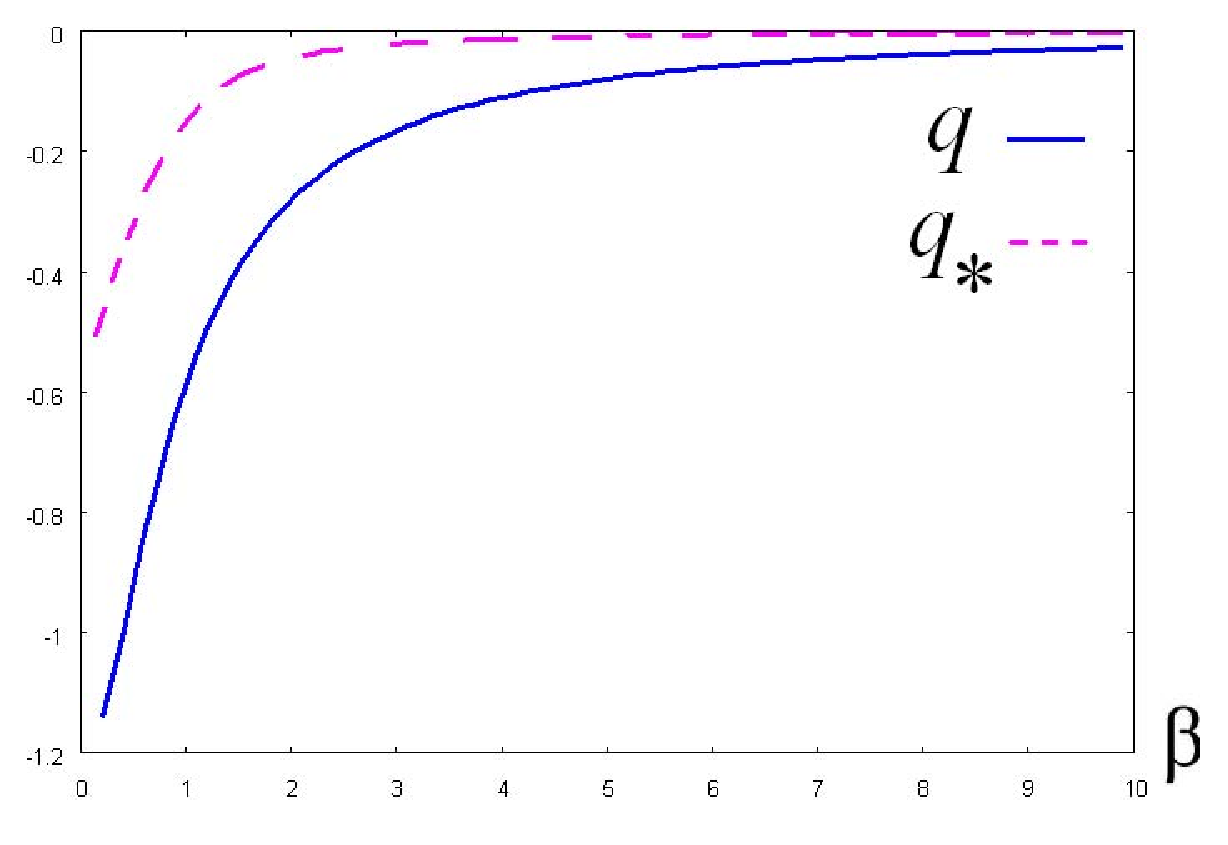
| (30) |
where .
VI Conclusion
A new parallel algorithm is developed for the simulation of the classical 3 spin glasses. It is shown that 3 spin glasses can be investigated by the help of an auxiliary Heisenberg Hamiltonian (1). The system of recurrent transcendental equations (3) and Silvester conditions (4) are obtained by using this Hamiltonian. Let us note that exactly similar equations of stationary points (3) also can be obtained if the full 3 Hamiltonian (see the first unnumbered formula) is used in the framework of short-range interaction model. That allows us step by step construct spin-chain of the specified length with taking into account the random surroundings. It is proved that at the limit of Birkhoff’s ergodic hypothesis performance, 3 spin glass can be generated by Hamiltonian of disordered 1 SSC with random environment. We have proved that it is always possible to construct spin-chain in any given random environment which will be in ground state energy (direct problem). We have also proved the inverse problem, namely, every spin-chain of the random environment can be surrounded by an environment so that it will be the solution in the ground state. In the work all the necessary numerical data were obtained by way of large number of parallel simulations of the auxiliary problem in order to construct all the statistical parameters of 3 spin glass at the limit of ergodicity of 1 SSCs nonideal ensemble. As numerical simulations show, the distributions of all statistical parameters become stable after independent calculations which are realized in parallel. The idea of 1 spin-chains parallel simulations, based on this simple and clear logic, greatly simplifies the calculations of 3 spin glasses which are still considered as a subset of difficult simulation problems. Let us note that computation of spin-spin interactions distribution function from the first principals of the classical mechanics is very important result of this work. As analysis show, the distribution is not an analytic function. It is from the class of Lévy functions which does not have variance and mean value .
Despite the absence of calculations by other methods, it is obvious that the developed scheme of calculations should differ from other algorithms, including the algorithms which are based on Monte Carlo simulation method [23], by the accuracy and efficiency. We were once again convinced in the accuracy and efficiency of the algorithm after analyzing the results of different numerical experiments by modeling the statistical parameters of 3 spin-glass system which are presented in figures 5 a, b and 6.
In the work a new way of partition function construction (configuration integral) is proposed in the form of one-dimensional integral of the energy distribution, which unlike the usual definitions does not include physically unrealizable spin-chains configurations (see difference of free energy derivatives on Fig. 8). It is obvious that the new definition of partition function is more correct and in addition it is very simple for computation.
Finally, the developed method can be generalized for the cases of external fields which will allow us investigate a large number of dynamical problems including critical properties of 3 classical spin glasses.
VII Acknowledgment
The work is partially supported by RFBR grants 10-01-00467-a, 11-01-0027-a.
References
References
- [1] Binder K and Young A 1986 Spin glasses: Experimental facts, theoretical concepts and open questions (Reviews of Modern Physics)
- [2] Mézard M, Parisi G and Virasoro M 1987 Spin Glass Theory and Beyond (World Scientific)
- [3] Young A 1998 Spin Glasses and Random Fields (World Scientific)
- [4] Fisch R and Harris A 1981 Spin-glass model in continuous dimensionality (Physical Review Letters)
- [5] Ancona-Torres C, Silevitch D, Aeppli G and Rosenbaum T 2008 Quantum and Classical Glass Transitions in LiHoxY1-xF4 (Physical Review Letters)
- [6] Bovier A 2006 Statistical Mechanics of Disordered Systems: A Mathematical Perspective (Cambridge Series in Statistical and Probabilistic Mathematics)
- [7] Tu Y, Tersoff J and Grinstein G 1998 Properties of a Continuous-Random-Network Model for Amorphous Systems (Physical Review Letters)
- [8] Chary K and Govil G 2008 NMR in Biological Systems: From Molecules to Human (Springer)
- [9] Baake E, Baake M and Wagner H 1997 Ising Quantum Chain is a Equivalent to a Model of Biological Evolution (Physical Review Letters)
- [10] Sherrington D and Kirkpatrick S 1975 A solvable model of a spin-glass (Physical Review Letters)
- [11] Derrida B 1981 Random-energy model: An exactly solvable model of disordered systems (Physical Review B)
- [12] Parisi G 1979 Infinite Number of Order Parameters for Spin-Glasses (Physical Review Letters)
- [13] Bray A and Moore M 1978 Replica-Symmetry Breaking in Spin-Glass Theories (Physical Review Letters)
- [14] Fernandez J and Sherrington D 1978 Randomly located spins with oscillatory interactions (Physical Review B)
- [15] Benamira F, Provost J and Valle G 1985 Separable and non-separable spin glass models (Journal de Physique)
- [16] Grensing D and Kühn R 1987 On classical spin-glass models (Journal de Physique)
- [17] Gevorkyan A et al. 2010 New Mathematical Conception and Computation Algorithm for Study of Quantum 3D Disordered Spin System Under the Influence of External Field (Transactions on computational science VII)
- [18] Gevorkyan A, Abajyan H and Sukiasyan H 2010 cond-mat.dis-nn1010.1623v1 (ArXiv)
- [19] Ibragimov I and Linnik Yu 1971 Independent and Stationary Sequences of Random Variebles (Wolters-Noordhoff Publishing Groningen)
- [20] Nolan J 2009 Stable Distributions: Models for Heavy Tailed Data (Birkhauser)
- [21] Wannier G 1987 Statistical Physics (Dover Publications)
- [22] Ziman J 1979 Models of Disorder: The Theoretical Physics of Homogeneously Disordered Systems (Cambridge Univ. Press)
- [23] Metropolis N, Rosenbluth A, Rosenbluth M, Teller A and Teller E 1953 Equation of State Calculations by Fast Computing Machines (J. Chem. Phys)