Next-to-leading order QCD predictions for the signal of Dark Matter and photon associated production at the LHC
Abstract
We study the potential of the LHC to discover the signal of Dark Matter associated production with a photon induced by a dimension six effective operator, including NLO QCD corrections. We investigate the main backgrounds from SM, i.e. boson and a photon associated production with invisible decay of boson, and boson and a jet production with the jet misidentified as a photon. We find that the distributions of the backgrounds decrease faster than that of the signal with increasing of the transverse momentum of the photon. The distributions of the backgrounds are almost flat in the full range of . In contrast, the signal lies mainly in the central region of . These characteristics may help to select the events in experiments. We show that in the parameter space allowed by the relic abundance constraint, which we have calculated at the NLO QCD level, the LHC with may discover this signal at the level after collecting an integrated luminosity of . On the other hand, if this signal is not observed at the LHC, we can set a lower limit on the new physics scale at the level.
pacs
12.38.Bx, 95.35.+d, 14.70.Bh, 14.65.JkI Introduction
Astrophysical and cosmological observations have confirmed the existence of Dark Matter (DM) in our universe[1] and the density of DM is much larger than that of the visible matter[2]. The relic abundance of DM favours a weakly interacting massive particles (WIMP). This kind of DM has been extensively studied in the literatures. Since there are no candidates of this kind of DM in the Standard Model (SM), any discovery of the signal of DM imply new physics.
In the region of DM accumulating, DM can annihilate into SM particles, such as photons, electrons and positrons. These produced particles can propagate through the interstellar space and be detected by experiments on the earth, such as PAMELA[3], ATIC[4], HESS[5] and Fermi LAT[6]. The detection of these signals is not conclusive evidence for DM, since it depends on the assumptions of the distribution of DM and the propagator model. Besides, other astrophysical interpretation can not be excluded. Another way to look for the signal of DM is to measure the recoil energy of nuclei caused by the elastic scattering of a WIMP off a nucleon, such as the experiments of DAMA[7], CDMS[8], CoGeNT[9] and XENON[10]. The DAMA and CoGeNT experiments favour a light DM with a mass around GeV. The CDMS and XENON experiments set upper limits on the WIMP and nucleon spin-dependent and spin-independent cross sections if the mass of the WIMP ranges from GeV to GeV. These experiments are passive and much time was spent in waiting for the collision with the DM. More active approach is to produce the DM in the laboratory directly, such as the Large Hadron Collider (LHC) if DM exists and has interactions with the SM particles. There are a lot of studies to search for DM at the LHC in varies of DM models[11, 12, 13, 14, 15, 16, 17, 18, 19, 20, 21, 22, 23, 24, 25, 26, 27, 28].
Because the LHC is a proton-proton collider, the QCD correction should be considered for any process if people want to make a reliable prediction. In this work, using model independent method, we investigate the possibility of discovering the DM in associated production with a photon induced by a dimension six effective operator at the next-to-leading (NLO) order QCD level, since this signal is clear and suffer from little backgrounds from the SM.
This paper is organized as follows. In section II, we describe the dimension six effective operator for this process. In section III, we calculate the relic abundance induced by this effective operator and find the allowed region for the mass and couplings of the DM. In section IV, we present the details of the NLO QCD corrections to the associated production of the DM and photon and discuss the dependence of the K-factor on the mass and couplings of the DM. In section V, we calculate the backgrounds in SM and analyze the discovery potential at the LHC. Conclusion will be given in section VI.
II Effective Operator
The DM studied in this work is a Dirac fermion, denoted by . It is a singlet under the SM gauge group . As a result, this kind of DM does not participate in any strong or electroweak interactions. In addition, we assume it couples with the SM quarks in the form
| (1) |
where is the new physics scale above which new particles should appear. This four-fermion operator has been considered in Refs.[29, 30, 21, 31] in discussing DM interactions. However, we will focus on the signal of DM and photon associated production at the LHC which has not been carefully investigated before. Moreover, we calculated the NLO QCD corrections for this process whose effects are important for research at the LHC. Note that the new physics scale can be viewed as the remnant of integrating the propagator between the SM particles and DM. Therefore, this operator is valid only if , where is the mass of DM and the center of mass energy of the collision. Generally, it is possible that at the LHC. However, the luminosity for the process drops very fast with the increasing of at the LHC with , which can be seen in Fig.1. Thus, we relax this limit in practical numerical calculation, where we set the default value of =500 GeV.


III Relic Abundance
The DM relic abundance is a precision observable in cosmology. The DM we choose to study can contribute to the relic abundance of cold Dark Matter (CDM). Combining WMAP data with the latest distance measurements from Baryon Acoustic Oscillations in the distribution of galaxies and Hubble constant measurements gives the constrain[32]
| (2) |
where is the CDM energy density of the Universe normalized by the critical density and is the scaled Hubble parameter.
The relic abundance can be calculated from the total annihilation cross section of DM. First, we give the LO total annihilation cross section as
| (3) |
where is the relative velocity between the DM. and are the numbers of color and flavor of quarks, respectively. This result agrees with that in Ref.[29].
The NLO corrections to the total annihilation cross section comprise of two parts: the one-loop virtual corrections and real gluon emission corrections. The results of virtual corrections are
| (4) |
where and is the n-dimensional LO total annihilation cross section
| (5) |
In obtaining the above results, we have renormalized the effective operator in the scheme. The results of real corrections are
| (6) |
Combining the two parts we get the NLO total annihilation cross section
| (7) |
The DM is moving at nonrelativistic velocities() when freezing out. Thus we can expand
| (8) |
where
| (9) |
in which is the K-factor of the DM annihilation cross section
| (10) |
The freezeout epoch is determined by[33]
| (11) |
where is the Planck mass. and is the number of relativistic degrees of freedom and effective number of relativistic degrees of freedom at the freeze-out temperature , respectively. The result for the relic abundance is
| (12) |
For most of the history of the universe all particle species had a common temperature, and can be replaced by . Requiring the DM relic abundance is in the region around the observed central value, the new physics scale of the effective operator is determined by the mass of the DM. We show this relation in Fig.2. When the parameters satisfy this relation, the NLO QCD K-factor is nearly 1.4. Comparing the LO result (blue band) and the NLO result (red band), we find that the NLO QCD correction increases the new physics scale by about 10%. Since we do not hold the point of view that the abundance of the WIMP is determined only by this one kind of DM, the regions below the red band are all allowed.

IV NLO QCD Corrections to DM and photon associated production
According to the operator in (1), the DM can be pair produced at hadron colliders. However, because DM can not decay into SM particles, such processes give just missing energy and no observable signals. As a result, we have to consider the process of DM associated production with a photon or a jet[30, 21, 31]. Though the cross section of associated production with a photon is less than that of associated production with a jet, the signal of this process is characteristic and bring with less backgrounds.
IV.1 LO calculation
We start from the leading order (LO) calculation. The LO Feynman diagrams for this process
| (13) |
are shown in Fig.3.

Because the DM does not interact with SM particles except for the quark fields in the operator (1), their contributions to the cross section can be factorized as
| (14) |
where . Therefore, the born matrix element can be written as
| (15) |
where the represent the standard matrix elements in our calculation which are defined as
| (16) |
The spin and color summed and averaged Born matrix element squared is
| (17) |
where and . Then the LO partonic cross section is
| (18) |
in which is the three particle final states phase space. After convoluting with the parton distribution functions (PDFs) , we obtain the LO cross section
| (19) |
.
IV.2 NLO results
The NLO QCD corrections involve the one-loop virtual gluon effects and contributions of real gluon and quark or antiquark emissions to leading order processes. To deal with ultraviolet (UV) and infrared (IR) (soft and collinear) divergences in our computation, we use dimensional regularization to regulate these divergences, and all divergences appear as with .

The virtual gluon corrections to DM and photon associated production consist of the self-energy, vertex and box diagrams, as shown in Fig.4. The UV divergences are canceled between the loop diagrams and counterterms which are determined in on-shell renormalization scheme for external fields and in scheme for coupling constants. The final virtual gluon corrections to the partonic cross section are
| (20) |
in which
where and
| (22) | |||||
We can also write Eq. (20) as
| (23) |
with
| (24) |
The first term in results from the renormalization of the four-fermion operator. The IR divergences remain after renormalization and have a structure predicted by other methods. They will cancel the IR divergences coming from real corrections.
A further contribution at hadron colliders arises from the process
| (25) |
which is illustrated in Fig.5. The effects of these loop-induced gg diagrams are one order of higher than that of diagrams, but they may be still important due to the large gluon PDFs at the LHC. However, the triangle and box diagrams in Fig.5 are both vanishing because of the color structure and charge conjugation symmetry, respectively.


The Feynman diagrams for the real gluon emission process
| (26) |
are shown in Fig.6. When performing the final states phase space integration, one encounters the soft and collinear singularities. We use the two cutoff phase space slicing method to separate the singular regions and perform the integration analytically in these regions[34]. Therefore, the real corrections are divided into three parts, i.e.,
| (27) |
where and denote the contributions from soft and hard collinear regions, respectively. The soft regions are defined by the energy of the emitted gluon , where is the soft cutoff parameter. The collinear regions are determined according to whether the Mandelstam variables , with , satisfy the collinear condition , where is the collinear cutoff parameter. The hard non-collinear part is finite and can be computed numerically.
The partonic cross section in soft regions can be factorized as
| (28) |
where is the integration over the phase space of the soft gluon
| (29) |
and the Eikonal factor is the amplitude squared in the soft limit apart from , expressed as
| (30) |
After integration over the soft gluon phase space, we get
| (31) |
where
| (32) |
In hard collinear regions of this process, the momentum of the gluon emitted from initial partons become collinear to the beam line. In this limit, the four-body matrix elements are approximated as follows:
| (33) |
in which, represents the fraction of initial partons’ momentum carried by . are the unregulated splitting functions in -dimensions which can be related to the usual Altarelli-Parisi splitting kernels as . In our case,
| (34) |
At the same limit, the four-body phase space can be written as
| (35) |
Therefore, we obtain
| (36) | |||||
To factorize the collinear singularity into the PDFs, we use scale dependent PDFs in the convention:
| (37) |
Now, we replace in the LO hadronic cross section (19) and combine the result with the hard collinear contribution (36). The resulting expression for the initial state collinear contribution is
| (38) | |||||
with
| (39) |
The functions are given by
| (40) |
with
| (41) |

A complete real correction includes also the (anti)quark emitted processes, as shown in Fig.7, such as
| (42) |
Their contribution can be obtained from the results of processes in (26) by crossing symmetry. Note that, when separating the singular phase space regions for these processes, one only needs to deal with the collinear divergences which can be totally absorbed into the redefinition of the PDFs in (37).
Finally, the NLO cross section for the process is
| (43) | |||||
where in suggests that the phase space integration is performed in the non-collinear regions. We have checked that
| (44) |
Therefore there are no singularities left now.
IV.3 Numerical results
In this subsection, we give the numerical results for the cross sections for DM and photon associated production at the LHC. In numerical calculation, we choose the CTEQ6L1 (CTEQ6M) PDF sets[35] and the corresponding strong coupling for the LO (NLO) calculations. The default factorization and renormalization scales, and , are set as . We choose the input parameters and unless otherwise specified which are allowed by the relic abundance constraint. The kinematic cuts
| (45) |
are applied in our numerical calculation. Here is the missing transverse momentum, defined as
| (46) |
where is the transverse momentum of the system of the DMs. Jets are defined by the requirements and . In order to avoid QED collinear divergences, we also require the photon to be isolated by the prescription[36]
| (47) |
where and .

In Fig.8 we show the cutoff parameter dependence of the NLO cross sections. The contribution of three-body final states includes the Born cross section, one-loop virtual corrections, soft and collinear limits of the cross section of four-body final states. The contribution of four-body final states consists in the cross section of four-body final states with the singular regions of the phase space sliced. The change of the NLO result is very slow, especially in the region , which indicates that it is reasonable to use the two cutoff phase space slicing method.

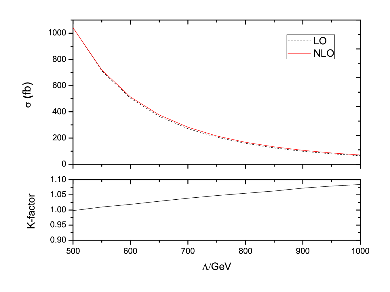
In Fig.9 we show the and dependence of the LO and NLO cross sections. The LO (NLO) cross sections decrease from to as increases from to . The corresponding K-factor, defined as the ratio of the NLO cross sections to the LO ones, varies from 0.99 to 1.02. The LO (NLO) cross sections decrease from to as increases from to . The corresponding K-factor varies from 1.00 to 1.08. The NLO QCD corrections are modest. However, the dependence of the NLO cross section on the factorization scale and renormalization scale is significantly reduced, as shown in Fig.10. This makes the theoretical prediction much more reliable.


V Backgrounds and discovery potential
The dominant SM backgrounds for this process include the processes and with the jet misidentified as a photon. The NLO QCD corrections to these processes are significant. We use the parton-level Monte Carlo program MCFM[37, 38, 39, 40] to estimate these backgrounds at NLO level. At the Tevatron, the probability that a jet fakes a photon is almost vanishing if the transverse momentum of the photon is larger then because in this situation the hits in the central preradiator chambers are counted and the prompt photon is distinguished from meson decays[41]. However, at the LHC, to remain on the safe side, we set , as suggested in Ref.[42].
Fig.11 shows the differential cross sections of both the signal and backgrounds as a function of and . It can be seen that the production is the main background. The distribution of the backgrounds decrease faster than that of the signal as the transverse momentum of the photon increases. Thus, the ratio of signal and background will increase if we set a larger cut.
Fig.12 shows the differential cross section of both the signal and backgrounds as a function of . The main background is the production, and it is almost flat in the full range of . In contrast, the signal concentrates in the central region of . This is a result of the scalar nature of the effective operator. These characteristics may help to select the events in experiments.


Fig.13 shows the integrated luminosity needed at the LHC with for a discovery () of the signal. For and , the integrated luminosities needed are around and , respectively. The situation at the LHC with is also shown in Fig.13. We find that the LHC may detect this signal once it collects an integrated luminosity of , which means that we may expect the observation of this signal at the early stage of the LHC. From an experimental point of view, if we discover this signal then we can set an upper limit for the new physics scale, which has been illustrated in Fig.14.


On the other hand, the LHC may not detect this signal at all. Thus we also present the exclusion limits of the new physics scale at the () level in Fig.14. We can see that the new physics scale is constrained to be larger than if the LHC with does not detect this signal after collecting an integrated luminosity of .
VI Conclusion
We have investigated DM annihilation and signal of DM and a photon associated production at the LHC induced by a dimension six effective operator at the NLO QCD level. We also study the main backgrounds from SM to this signal, i.e. boson and a photon associated production with invisible decay of boson, and boson and a jet production with the jet misidentified as a photon. We find that the distributions of the backgrounds decrease faster than that of the signal with increasing of the transverse momentum of the photon. The distributions of the backgrounds are almost flat in the full range of . In contrast, the signal lies mainly in the central region of . These characteristics may help to select the events in experiments. We show that in the parameter space allowed by the relic abundance constraint, which we have calculated at the NLO QCD level, the LHC with may discovery this signal at the level after collecting an integrated luminosity of . On the other hand, if this signal is not observed at the LHC, we set a lower limit on the new physics scale at the level.
Acknowledgements.
We would like to thank Qing-Hong Cao for useful discussion. This work was supported in part by the National Natural Science Foundation of China, under Grants No. 11021092 and No. 10975004.References
- [1] G. Jungman, M. Kamionkowski, and K. Griest, Phys. Rept. 267, 195 (1996), eprint hep-ph/9506380.
- [2] E. Komatsu et al. (WMAP), Astrophys. J. Suppl. 180, 330 (2009), eprint 0803.0547.
- [3] O. Adriani et al. (PAMELA), Phys. Rev. Lett. 105, 121101 (2010), eprint 1007.0821.
- [4] J. Chang et al., Nature 456, 362 (2008).
- [5] F. Aharonian et al. (H.E.S.S.), Phys. Rev. Lett. 101, 261104 (2008), eprint 0811.3894.
- [6] A. A. Abdo et al. (The Fermi LAT), Phys. Rev. Lett. 102, 181101 (2009), eprint 0905.0025.
- [7] R. Bernabei et al. (DAMA), Eur. Phys. J. C56, 333 (2008), eprint 0804.2741.
- [8] Z. Ahmed et al. (CDMS), Phys. Rev. Lett. 102, 011301 (2009), eprint 0802.3530.
- [9] C. E. Aalseth et al. (CoGeNT), Phys. Rev. Lett. 106, 131301 (2011), eprint 1002.4703.
- [10] E. Aprile et al. (XENON100), Phys. Rev. Lett. 105, 131302 (2010), eprint 1005.0380.
- [11] O. Buchmueller et al. (2011), eprint 1106.2529.
- [12] T. Li, J. A. Maxin, D. V. Nanopoulos, and J. W. Walker (2011), eprint 1106.1165.
- [13] S. Profumo (2011), eprint 1105.5162.
- [14] G. Belanger, S. Kraml, and A. Lessa (2011), eprint 1105.4878.
- [15] J. Kile and A. Soni (2011), eprint 1104.5239.
- [16] S. Akula, D. Feldman, Z. Liu, P. Nath, and G. Peim (2011), eprint 1103.5061.
- [17] D. Feldman, K. Freese, P. Nath, B. D. Nelson, and G. Peim (2011), eprint 1102.2548.
- [18] Y. Bai and H.-C. Cheng, JHEP 06, 021 (2011), eprint 1012.1863.
- [19] I. Gogoladze, R. Khalid, Y. Mimura, and Q. Shafi, Phys. Rev. D83, 095007 (2011), eprint 1012.1613.
- [20] K. Cheung, K. Mawatari, E. Senaha, P.-Y. Tseng, and T.-C. Yuan, JHEP 10, 081 (2010), eprint 1009.0618.
- [21] J. Goodman et al., Phys. Rev. D82, 116010 (2010), eprint 1008.1783.
- [22] G. Bertone, D. G. Cerdeno, M. Fornasa, R. Ruiz de Austri, and R. Trotta, Phys. Rev. D82, 055008 (2010), eprint 1005.4280.
- [23] G. F. Giudice, T. Han, K. Wang, and L.-T. Wang, Phys. Rev. D81, 115011 (2010), eprint 1004.4902.
- [24] T. Li and W. Chao, Nucl. Phys. B843, 396 (2011), eprint 1004.0296.
- [25] M. Beltran, D. Hooper, E. W. Kolb, Z. A. C. Krusberg, and T. M. P. Tait, JHEP 09, 037 (2010), eprint 1002.4137.
- [26] H. Zhang, C. S. Li, Q.-H. Cao, and Z. Li, Phys. Rev. D82, 075003 (2010), eprint 0910.2831.
- [27] N. Arkani-Hamed and N. Weiner, JHEP 12, 104 (2008), eprint 0810.0714.
- [28] D. Fargion, M. Y. Khlopov, R. V. Konoplich, and R. Mignani, Phys. Rev. D54, 4684 (1996).
- [29] M. Beltran, D. Hooper, E. W. Kolb, and Z. A. C. Krusberg, Phys. Rev. D80, 043509 (2009), eprint 0808.3384.
- [30] Q.-H. Cao, C.-R. Chen, C. S. Li, and H. Zhang (2009), eprint 0912.4511.
- [31] Y. Bai, P. J. Fox, and R. Harnik, JHEP 12, 048 (2010), eprint 1005.3797.
- [32] N. Jarosik et al., Astrophys. J. Suppl. 192, 14 (2011), eprint 1001.4744.
- [33] E. W. Kolb and M. S. Turner, Front.Phys. 69, 1 (1990).
- [34] B. W. Harris and J. F. Owens, Phys. Rev. D65, 094032 (2002), eprint hep-ph/0102128.
- [35] J. Pumplin et al., JHEP 07, 012 (2002), eprint hep-ph/0201195.
- [36] S. Frixione, Phys. Lett. B429, 369 (1998), eprint hep-ph/9801442.
- [37] J. M. Campbell, R. K. Ellis, and C. Williams (2011), eprint 1105.0020.
- [38] U. Baur, T. Han, and J. Ohnemus, Phys. Rev. D57, 2823 (1998), eprint hep-ph/9710416.
- [39] J. Ohnemus, Phys. Rev. D47, 940 (1993).
- [40] W. T. Giele, E. W. N. Glover, and D. A. Kosower, Nucl. Phys. B403, 633 (1993), eprint hep-ph/9302225.
- [41] D. E. Acosta et al. (CDF II), Phys. Rev. Lett. 94, 041803 (2005), eprint hep-ex/0410008.
- [42] U. Baur and E. L. Berger, Phys. Rev. D47, 4889 (1993).