Stochastic convex optimization with bandit feedback

Alekh Agarwal^†

Dean P. Foster^⋆

Daniel Hsu^‡

Sham M. Kakade^⋆,‡

Alexander Rakhlin^⋆

Department of EECS^†	Department of Statistics^⋆	Microsoft Research^‡
University of California, Berkeley	University of Pennsylvania	New England
Berkeley, CA 94720	Philadelphia, PA 19104	Cambridge, MA 02142

Abstract

This paper addresses the problem of minimizing a convex, Lipschitz function $f$ over a convex, compact set $\mathcal{X}$ under a stochastic bandit feedback model. In this model, the algorithm is allowed to observe noisy realizations of the function value $f(x)$ at any query point $x\in\mathcal{X}$ . The quantity of interest is the regret of the algorithm, which is the sum of the function values at algorithm’s query points minus the optimal function value. We demonstrate a generalization of the ellipsoid algorithm that incurs $\widetilde{\mathcal{O}}(\poly(d)\sqrt{T})$ regret. Since any algorithm has regret at least $\Omega(\sqrt{T})$ on this problem, our algorithm is optimal in terms of the scaling with $T$ .

1 Introduction

The classical multi-armed bandit problem, formulated by Robbins in 1952, is arguably the most basic setting of sequential decision-making under uncertainty. Upon choosing one of $k$ available actions (“arms”), the decision-maker observes an i.i.d. realization of the arm’s cost drawn according to a distribution associated with the arm. The performance of an allocation rule (algorithm) in sequentially choosing the arms is measured by regret, that is the difference between the expected costs of the chosen actions as compared to the expected cost of the best action. Various extensions of the classical formulation have received much attention in recent years. In particular, research has focused on the development of optimal and efficient algorithms for multi-armed bandits with large or even infinite action spaces, relying on various assumptions on the structure of costs (rewards) over the action space. When such a structure is present, the information about the cost of one arm propagates to other arms as well, making the problem tractable. For instance, the mean cost function is assumed to be linear in the paper [9], facilitating global “sharing of information” over a compact convex set of actions in a $d$ -dimensional space. A Lipschitz condition on the mean cost function allows a local propagation of information about the arms, as costs cannot change rapidly in a neighborhood of an action. This has been exploited in a number of works, notably [2, 13, 14]. Instead of the Lipschitz condition, Srinivas et al. [18] exploit the structure of Gaussian processes, focusing on the notion of the effective dimension. These various “non-parametric” bandit problems typically suffer from the curse of dimensionality, that is, the best possible convergence rates (after $T$ queries) are typically of the form $T^{\alpha}$ , with the exponent $\alpha$ approaching $1$ for large dimension $d$ .

The question addressed in the present paper is: How can we leverage convexity of the mean cost function as a structural assumption? The main contribution of the paper is an algorithm which achieves, with high probability, an $\tilde{O}(\text{poly}(d)\sqrt{T})$ regret after $T$ requests. This result holds for all convex Lipschitz mean cost functions. We remark that the rate does not deteriorate with $d$ (except in the multiplicative term) implying that convexity is a strong structural assumption which turns “non-parametric” Lipschitz problems into “parametric”. Nevertheless, convexity is a very natural and basic assumption, and applications of our method are, therefore, abundant. Let us also remark that $\Omega(\sqrt{dT})$ lower bounds have been shown for linear mean cost functions [9], making our algorithm optimal up to factors polynomial in the dimension $d$ and logarithmic in the number of iterations $T$ .

We note that our work focuses on the so-called stochastic bandits setting, where the observed costs of an action are i.i.d. draws from a fixed distribution. A parallel line of literature focuses on the more difficult adversarial setting where the costs of actions change arbitrarily from round to round. Leveraging structure in non-stochastic bandit settings is more complex, and is not a goal of this paper.

We start by defining some notation and the problem setup below. The next section will survey related prior works and describe their connections with our work in Section 3. Section 4 gives the algorithm and analysis for the special case of univariate optimization. The algorithm for higher dimensions and its analysis are given in Section 5.

Notation and setup:

Let $\mathcal{X}$ be a compact and convex subset of $\mathbb{R}^{d}$ , and let $f\colon\mathcal{X}\to\mathbb{R}$ be a $1$ -Lipschitz convex function on $\mathcal{X}$ , so $f(x)-f(x^{\prime})\leq\|x-x^{\prime}\|$ for all $x,x^{\prime}\in\mathcal{X}$ . We assume that $\mathcal{X}$ is specified in a way so that an algorithm can efficiently construct the smallest Euclidean ball containing the set. Furthermore, we assume the algorithm has noisy black-box access to $f$ . Specifically, the algorithm is allowed to query the value of $f$ at any $x\in\mathcal{X}$ , and the response to the query $x$ is

y=f(x)+\varepsilon

where $\varepsilon$ is an independent $\sigma$ -subgaussian random variable with mean zero: ${\mathbb{E}}[\exp(\lambda\varepsilon)]\leq\exp(\lambda^{2}\sigma^{2}/2)$ for all $\lambda\in\mathbb{R}$ . The algorithm incurs a cost $f(x)$ for each query $x$ . The goal of the algorithm is to minimize its regret: after making $T$ queries $x_{1},\dotsc,x_{T}\in\mathcal{X}$ , the regret of the algorithm is

R_{T}=\sum_{t=1}^{T}\bigl(f(x_{t})-f(x^{*})\bigr)

where $x^{*}$ is the minimizer of $f$ over $\mathcal{X}$ (we do not require uniqueness of $x^{*}$ ).

Since we observe noisy function values, our algorithms will make multiple queries of $f$ at the same point. We will construct an average and confidence interval (henceforth CI) around the average for the function values at points queried by the algorithm. We will use the notation $\operatorname{LB}_{\gamma_{i}}(x)$ and $\operatorname{UB}_{\gamma_{i}}(x)$ to denote the lower and upper bounds of a CI of width $\gamma_{i}$ for the function estimate of a point $x$ . We will say that CI’s at two points are $\gamma$ -separated if $\operatorname{LB}_{\gamma_{i}}(x)\geq\operatorname{UB}_{\gamma_{i}}(y)+\gamma$ or $\operatorname{LB}_{\gamma_{i}}(y)\geq\operatorname{UB}_{\gamma_{i}}(x)+\gamma$ .

2 Related work

Asymptotic rates of $\mathcal{O}(\sqrt{T})$ have been previously achieved by Cope [8] for unimodal functions under stringent conditions (smoothness and strong convexity of the mean cost function, in addition to the unconstrained optimum being achieved inside the constraint set). The method employed by the author is a variant of the classical Kiefer-Wolfowitz procedure [12] for estimation of an optimum point. Further, the rate $\tilde{O}(\sqrt{T})$ has been achieved in Auer et al. [3] for a one-dimensional non-convex problem with finite number of optima. The result assumes continuous second derivatives of the mean function, not vanishing at the optimum, while the first derivative is assumed to be zero at the optima. The method is based on discretizing the interval and does not exploit convexity. Yu and Mannor [19] recently studied unimodal bandits, but they only consider one-dimensional and graph-structured settings. Bubeck et al. [6] consider the general setup of $\mathcal{X}$ -armed bandits with Lipschitz mean cost functions and their algorithm does give $\mathcal{O}(c(d)\sqrt{T})$ regret for a dimension dependent constant $c(d)$ in some cases when the problem has a near-optimality dimension of 0. However, not all convex, Lipschitz functions satisfy this condition, and $c(d)$ can grow exponentially in $d$ even in these special cases.

The case of convex, Lipschitz cost functions has been looked at in the harder adversarial model [10, 13] by constructing one-point gradient estimators. However, the best-known regret bounds for these algorithms are $\mathcal{O}(T^{3/4})$ . Agarwal et al. [1] show a regret bound of $\mathcal{O}(\sqrt{T})$ in the adversarial setup, when two evaluations of the same function are allowed, instead of just one. However, this does not include the stochastic bandit optimization setting since each function evaluation in the stochastic case is corrupted with independent noise, violating the critical requirement of a bounded gradient estimator that their algorithm exploits. Indeed, applying their result in our setup yields a regret bound of $\mathcal{O}(T^{3/4})$ .

A related line of work attempts to solve convex optimization problems by instead posing the problem of finding a feasible point from a convex set. Different oracle models of specifying the convex set correspond to different optimization settings. The bandit setting is identical to finding a feasible point, given only a membership oracle for the convex set. Since we get only noisy function evaluations, we in fact only have access to a noisy membership oracle. While there are elegant solutions based on random walks in the easier separation oracle model [5], the membership oracle setting has been mostly studied in the noiseless setting only and uses much more complex techniques building on the seminal work of Nemirovski and Yudin [15]. The techniques have the additional drawback that they do not guarantee a low regret since the methods often explore aggressively.

We observe that the problem addressed in this paper is closely related to noisy zero-th order (also called derivative-free) convex optimization, whereby the algorithm queries a point of the domain and receives a noisy value of the function. Given $\epsilon>0$ , such algorithms are guaranteed to produce an $\epsilon$ -minimizer at the end of $T$ iterations. While the literature on stochastic optimization is vast, we emphasize that an optimization guarantee does not necessarily imply a bound on regret. We explain this point in more detail below.

Since $f$ is convex by assumption, the average $\bar{x}_{T}=\frac{1}{T}\sum_{t=1}^{T}x_{t}$ must satisfy $f(\bar{x}_{T})-f(x^{*})\leq R_{T}/T$ (by Jensen’s inequality). That is, a method guaranteeing small regret is also an optimization algorithm. The converse, however, is not necessarily true. Suppose an optimization algorithm queries $T$ points of the domain and then outputs a candidate minimizer $x^{*}_{T}$ . Without any assumption on the behavior of the optimization method nothing can be said about the regret it suffers over $T$ iterations. In fact, depending on the particular setup, an optimization method might prefer to spend time querying far from the minimum of the function (that is, explore) and then output the solution at the last step. Guaranteeing a small regret typically involves a more careful balancing of exploration and exploitation. This distinction between arbitrary optimization schemes and anytime methods is discussed further in the paper [17].

We note that most of the existing approaches to derivative-free optimization outlined in the recent book [7] typically search for a descent or sufficient descent direction and then take a step in this direction. However, most convergence results are asymptotic and do not provide concrete rates even in an optimization error setting. The main emphasis is often on global optimization of non-convex functions, while we are mainly interested in convex functions in this work. Nesterov [16] recently analyzes schemes similar to that of Agarwal et al. [1] with access to noiseless function evaluations, showing $\mathcal{O}(\sqrt{dT})$ convergence for non-smooth functions and accelerated schemes for smooth mean cost functions. However, when analyzed in a noisy evaluation setting, his rates suffer from the degradation as those of Agarwal et al. [1].

3 Outline of our approach

The close relationship between convex optimization and the regret-minimization problem suggests a plan of attack: Check whether existing stochastic zeroth order optimization methods (that is, methods that only query the oracle for function values), in fact, minimize regret. Two types of methods for stochastic zeroth order convex optimization are outlined in Nemirovski and Yudin [15, Chapter 9]. The first approach uses the noisy function values to estimate a gradient direction at every step, and then passes this information to a stochastic first-order method. The second approach is to use the zeroth order information to estimate function values and pass this information to a noiseless zeroth order method. Nemirovski and Yudin argue that the latter approach has greater stability when compared to the former. Indeed, for a gradient estimate to be meaningful, function values should be sampled close to the point of interest, which, in turn, results in a poor quality of the estimate. This tension is also the source of difficulty in minimizing regret with a convex mean cost function.

Owing to the insights of Nemirovski and Yudin [15], we opt for the second approach, giving up the idea of estimating the first-order information. The main novel tool of the paper is a “center-point device” that allows to quickly detect that the optimization method might be paying high regret and to act on this information. Unlike discretization-based methods, the proposed algorithm uses convexity in a crucial way. We first demonstrate the device on one-dimensional problems, where the solution is clean and intuitive. We then develop a version of the algorithm for higher dimensions, basing our construction on the beautiful zero-th order optimization method of Nemirovski and Yudin [15]. Their method does not guarantee vanishing regret by itself, and a careful fusion of this algorithm with our center-point device is required. The overall approach would be to use center-point device in conjunction with a modification of the classical ellipsoid algorithm.

To motivate the center-point device, consider the following situation. Suppose $f$ is the unknown function on $\mathcal{X}=[0,1]$ , and assume for now that it is linear with a slope $T^{-1/3}$ . Let us sample function values at $x=1/4$ and $x=3/4$ . To even distinguish the slope from a slope $-T^{-1/3}$ (which results in a minimizer on the opposite side of $\mathcal{X}$ ), we need $O(T^{2/3})$ points. If the function $f$ is linear indeed, we only incur $O(T^{1/3})$ regret on these rounds. However, if instead $f$ is a quadratic dipping between the sampled points, we incur regret of $O(T^{2/3})$ . To quickly detect that the function is not flat between the two sampled points, we additionally sample at $x=1/2$ . The center point acts as a sentinel: if it is recognized that the function value at the center point is noticeably below the other two values, the region $[0,1/4]\cup[3/4,1]$ can be discarded. If it is recognized that the value of $f$ either at $x=1/4$ or at $x=3/4$ is greater than others, then either $[0,1/4]$ or $[3/4,1]$ can be discarded. Finally, if $f$ at all three points appears to be similar at a given scale, we have a certificate that the algorithm is not paying regret larger than this scale per query. The remaining argument proceeds similarly to the binary search or the method of centers of gravity: since a constant portion of the set is discarded every time, it only requires a logarithmic number of “cuts”. We remark that this novelty is indeed in ensuring that regret is kept small in the process; a simpler algorithm which does not query the center is sufficient to guarantee a small optimization error but incurs a large regret on examples of the form sketched above.

In the next section we present the algorithm that results from the above ideas for one-dimensional convex optimization. The general case in higher dimensions is presented in Section 5.

4 One-dimensional case

We start with a specialization of the setting to 1-dimension to illustrate some of the key ideas including the center-point device. We assume without loss of generality that the domain $\mathcal{X}=[0,1]$ , and $f(x)\in[0,1]$ (the latter can be achieved by pinning $f(x^{*})=0$ since $f$ is 1-Lipschitz).

4.1 Algorithm description

Algorithm 1 One-dimensional stochastic convex bandit algorithm

0: noisy black-box access to

f\colon[0,1]\to\mathbb{R}

, total number of queries allowed

T

1: Let

l_{1}:=0

and

r_{1}:=1

2: for epoch

\tau=1,2,\dotsc

3: Let

w_{\tau}:=r_{\tau}-l_{\tau}

4: Let

x_{l}:=l_{\tau}+w_{\tau}/4

x_{c}:=l_{\tau}+w_{\tau}/2

, and

x_{r}:=l_{\tau}+3w_{\tau}/4

5: for round

i=1,2,\dotsc

6: Let

\gamma_{i}:=2^{-i}

7: For each

x\in\{x_{l},x_{c},x_{r}\}

, query

f(x)

\frac{2\sigma}{\gamma_{i}^{2}}\log T

times.

8: if

\max\{\operatorname{LB}_{\gamma_{i}}(x_{l}),\operatorname{LB}_{\gamma_{i}}(x_{r})\}\geq\min\{\operatorname{UB}_{\gamma_{i}}(x_{l}),\operatorname{UB}_{\gamma_{i}}(x_{r})\}+\gamma_{i}

then

9: {Case 1: CI’s at

x_{l}

and

x_{r}

are

\gamma_{i}

separated}

10: if

\operatorname{LB}_{\gamma_{i}}(x_{l})\geq\operatorname{LB}_{\gamma_{i}}(x_{r})

then let

l_{\tau+1}:=x_{l}

and

r_{\tau+1}:=r_{\tau}

11: if

\operatorname{LB}_{\gamma_{i}}(x_{l})<\operatorname{LB}_{\gamma_{i}}(x_{r})

then let

l_{\tau+1}:=l_{\tau}

and

r_{\tau+1}:=x_{r}

12: Continue to epoch

\tau+1

13: else if

\max\{\operatorname{LB}_{\gamma_{i}}(x_{l}),\operatorname{LB}_{\gamma_{i}}(x_{r})\}\geq\operatorname{UB}_{\gamma_{i}}(x_{c})+\gamma_{i}

then

14: {Case 2: CI’s at

x_{c}

and

x_{l}

x_{r}

are

\gamma_{i}

separated}

15: if

\operatorname{LB}_{\gamma_{i}}(x_{l})\geq\operatorname{LB}_{\gamma_{i}}(x_{r})

then let

l_{\tau+1}:=x_{l}

and

r_{\tau+1}:=r_{\tau}

16: if

\operatorname{LB}_{\gamma_{i}}(x_{l})<\operatorname{LB}_{\gamma_{i}}(x_{r})

then let

l_{\tau+1}:=l_{\tau}

and

r_{\tau+1}:=x_{r}

17: Continue to epoch

\tau+1

18: end if

19: end for

20: end for

Algorithm 1 proceeds in a series of epochs demarcated by a working feasible region (the interval $[l_{\tau},r_{\tau}]$ in epoch $\tau$ ). In each epoch, the algorithm aims to discard a portion of the working feasible region determined to only contain suboptimal points. To do this, the algorithm repeatedly makes noisy queries to $f$ at three different points in the working feasible region. Each epoch is further subdivided into rounds, where we query the function $(2\sigma\log T)/\gamma_{i}^{2}$ times in round $i$ at each of the points. By Hoeffding’s inequality, this implies that we know the function value to within $\gamma_{i}$ with high probability. The value $\gamma_{i}$ is halved at every round so that the algorithm can stop the epoch with the minimal number of queries that suffice to resolve the difference between function values at any two of $x_{l},x_{c},x_{r}$ , ensuring a low regret regret in each epoch. At the end of an epoch $\tau$ , the working feasible region is reduced to a subset $[l_{\tau+1},r_{\tau+1}]\subset[l_{\tau},r_{\tau}]$ of the current region for the next epoch $\tau+1$ , and this reduction is such that the new region is smaller in size by a constant fraction. This geometric rate of reduction guarantees that only a small number of epochs can occur before the working feasible region only contains near-optimal points.

In order for the algorithm to identify a sizable portion of the working feasible region containing only suboptimal points to discard, the queries in each epoch should be suitably chosen, and the convexity of $f$ must be judiciously exploited. To this end, the algorithm makes its queries at three equally-spaced points $x_{l}<x_{c}<x_{r}$ in the working feasible region.

Case 1:: If the confidence intervals around $f(x_{l})$ and $f(x_{r})$ are sufficiently separated, then the algorithm can identify a subset of the feasible region (either to the left of $x_{l}$ or to the right of $x_{r}$ ) that contains no near-optimal points—i.e., that every point $x$ in the subset has $f(x)\gg f(x^{*})$ . This subset, which is a fourth of the working feasible region by construction is then discarded and the algorithm continues to the next epoch. This case is depicted in Figure 1.

Figure 1: Two possible configurations when the algorithm enters case 1.
Case 2:: If the above deduction cannot be made, the algorithm looks at the confidence interval around $f(x_{c})$ . If this interval is sufficiently below at least one of the other intervals (for $f(x_{l})$ or $f(x_{r})$ ), then again the algorithm can identify a quartile that contains no near-optimal points, and this quartile can then be discarded before continuing to the next epoch. One possible arrangement of CI’s for this case is shown in Figure 3.
Case 3:: Finally, if none of the earlier cases is true, then the algorithm is assured that the function is sufficiently flat on working feasible region and hence it has not incurred much regret so far. The algorithm continues the epoch, with an increased number of queries to obtain smaller confidence intervals at each of the three points. An example arrangement of CI’s for this case is shown in Figure 3.

Figure 2: One of the possible configurations when the algorithm enters Case 2.

Figure 3: Configuration of the confidence intervals in Case 3 of Algorithm 1.

4.2 Analysis

The analysis of Algorithm 1 relies on the function values being contained in the confidence intervals we construct at each round of each epoch. To avoid having probabilities throughout our analysis, we define an event $\mathcal{E}$ where at each epoch $\tau$ , and each round $i$ , $f(x)\in[\operatorname{LB}_{\gamma_{i}}(x),\operatorname{UB}_{\gamma_{i}}(x)]$ for $x\in\{x_{l},x_{c},x_{r}\}$ . We will carry out the remainder of the analysis conditioned on $\mathcal{E}$ and bound the probability of $\mathcal{E}^{c}$ at the end.

The following theorem bounds the regret incurred by Algorithm 1. We note that the regret would be maintained in terms of the points $x_{t}$ queried by the algorithm at time $t$ . Within any given round, the order of queries is immaterial to the regret.

Theorem 1 (Regret bound for Algorithm 1).

Suppose Algorithm 1 is run on a convex, 1-Lipschitz function $f$ bounded in [0,1]. Suppose the noise in observations is i.i.d. and $\sigma$ -subgaussian. Then with probability at least $1-1/T$ we have

\sum_{t=1}^{T}f(x_{t})-f(x^{*})\leq 108\sqrt{\sigma T\log T}\log_{4/3}\left(\frac{T}{8\sigma\log T}\right).

Remarks:

As stated Algorithm 1 and Theorem 1 assume knowledge of $T$ , but we can make the algorithm adaptive to $T$ by a standard doubling argument. We remark that $\mathcal{O}(\sqrt{T})$ is the smallest possible regret for any algorithm even with noisy gradient information. Hence, this result shows that for purposes of regret, noisy zeroth order information is no worse than noisy first-order information apart from logarithmic factors. We also observe that at the end of the procedure, the mid-point $x_{c}$ of the working feasible region $[l_{\tau},r_{\tau}]$ where $\tau$ was the last epoch, has an optimization error of at most $\tilde{\mathcal{O}}(1/\sqrt{T})$ . This is unlike noisy first-order methods where all the iterates have to be averaged in order to get a point with low optimization error.

The theorem is proved via a series of lemmas in the next few sections. The key idea is to show that the regret on any epoch is small and the total number of epochs is bounded. To bound the per-epoch regret, we will show that the total number of queries made on any epoch depends on how close to flat the function is on the working feasible region. Thus we either take a long time, but the function is very flat, or we stop early when the function has sufficient slope, never accruing too much regret.

4.2.1 Bounding the regret in one epoch

We start by showing that each reduction in the working feasible region after each epoch never discards near-optimal points.

Lemma 1.

If epoch $\tau$ ends in round $i$ , then the interval $[l_{\tau+1},r_{\tau+1}]$ contains every $x\in[l_{\tau},r_{\tau}]$ such that $f(x)\leq f(x^{*})+\gamma_{i}$ . In particular, $x^{*}\in[l_{\tau},r_{\tau}]$ for all epochs $\tau$ .

Proof.

Suppose epoch $\tau$ terminates in round $i$ via case 1. This means that either $\operatorname{LB}_{\gamma_{i}}(x_{l})\geq\operatorname{UB}_{\gamma_{i}}(x_{r})+\gamma_{i}$ or $\operatorname{LB}_{\gamma_{i}}(x_{r})\geq\operatorname{UB}_{\gamma_{i}}(x_{l})+\gamma_{i}$ . Consider the former case (the argument for the latter is analogous). This implies

f(x_{l})\geq f(x_{r})+\gamma_{i}.

(1)

We need to show that every $x\in[l_{\tau},l_{\tau+1}]=[l_{\tau},x_{l}]$ has $f(x)\geq f(x^{*})+{\gamma_{i}}$ . So pick $x\in[l_{\tau},x_{l}]$ so that $x_{l}\in[x,x_{r}]$ . Then $x_{l}=tx+(1-t)x_{r}$ for some $0\leq t\leq 1$ , so by convexity,

f(x_{l})\leq tf(x)+(1-t)f(x_{r}),

which in turn implies

	$\displaystyle f(x)$	$\displaystyle\geq f(x_{r})+\frac{f(x_{l})-f(x_{r})}{t}$
		$\displaystyle\geq f(x_{r})+\frac{\gamma_{i}}{t}\qquad\mbox{using Equation~\ref{eqn:1dgammasep}}$
		$\displaystyle\geq f(x^{*})+\gamma_{i}\qquad\mbox{since $t\leq 1$}$

as required.

Now suppose epoch $\tau$ terminates in round $i$ via case 2. This means

\max\{\operatorname{LB}_{\gamma_{i}}(x_{l}),\operatorname{LB}_{\gamma_{i}}(x_{r})\}\geq\operatorname{UB}_{\gamma_{i}}(x_{c})+\gamma_{i}.

Suppose $\operatorname{LB}_{\gamma_{i}}(x_{l})\geq\operatorname{LB}_{\gamma_{i}}(x_{r})$ (the argument for the case $\operatorname{LB}_{\gamma_{i}}(x_{l})<\operatorname{LB}_{\gamma_{i}}(x_{r})$ is analogous). The above inequality implies

f(x_{l})\geq f(x_{c})+\gamma_{i}.

We need to show that every $x\in[l_{\tau},l_{\tau+1}]=[l_{\tau},x_{l}]$ has $f(x)\geq f(x^{*})+\gamma_{i}$ . But the same argument as given in case 1, with $x_{r}$ replaced with $x_{c}$ , gives the required claim.

The fact that $x^{*}\in[l_{\tau},r_{\tau}]$ for all epochs $\tau$ follows by induction. ∎

The next two lemmas bound the regret incurred in any single epoch. To show this, we first establish that an algorithm incurs low regret in a round as long as it does not end an epoch. Then, as a consequence of the doubling trick, we show that the regret incurred in an epoch is on the same order as that incurred in the last round of the epoch.

Lemma 2 (Certificate of low regret).

If epoch $\tau$ continues from round $i$ to round $i+1$ , then the regret incurred in round $i$ is at most

\frac{72\sigma\log T}{\gamma_{i}}.

Remark 1.

A more detailed argument shows that the regret incurred is, in fact, at most $54\sigma\log T/\gamma_{i}$ .

Proof.

The regret incurred in round $i$ of epoch $\tau$ is

\frac{2\sigma\log T}{\gamma_{i}^{2}}\cdot\Bigl((f(x_{l})-f(x^{*}))+(f(x_{c})-f(x^{*}))+(f(x_{r})-f(x^{*}))\Bigr)

so it suffices to show that

f(x)\leq f(x^{*})+12\gamma_{i}

for each $x\in\{x_{l},x_{c},x_{r}\}$ .

The algorithm continues from round $i$ to round $i+1$ iff

\max\{\operatorname{LB}_{\gamma_{i}}(x_{l}),\operatorname{LB}_{\gamma_{i}}(x_{r})\}<\min\{\operatorname{UB}_{\gamma_{i}}(x_{l}),\operatorname{UB}_{\gamma_{i}}(x_{r})\}+\gamma_{i}

and

\max\{\operatorname{LB}_{\gamma_{i}}(x_{l}),\operatorname{LB}_{\gamma_{i}}(x_{r})\}<\operatorname{UB}_{\gamma_{i}}(x_{c})+\gamma_{i}.

This implies that $f(x_{l})$ , $f(x_{c})$ , and $f(x_{r})$ are contained in an interval of width at most $3\gamma_{i}$ (recall Figure 3).

By Lemma 1, we have $x^{*}\in[l_{\tau},r_{\tau}]$ . Assume $x^{*}\leq x_{c}$ (the case $x^{*}>x_{c}$ is analogous). There exists $t\geq 0$ such that $x^{*}=x_{c}+t(x_{c}-x_{r})$ , so

x_{c}=\frac{1}{1+t}x^{*}+\frac{t}{1+t}x_{r}.

Note that $t\leq 2$ because $|x_{c}-l_{\tau}|=w_{\tau}/2$ and $|x_{r}-x_{c}|=w_{\tau}/4$ , so

t=\frac{|x^{*}-x_{c}|}{|x_{r}-x_{c}|}\leq\frac{|l_{\tau}-x_{c}|}{|x_{r}-x_{c}|}=\frac{w_{\tau}/2}{w_{\tau}/4}=2.

By convexity,

f(x_{c})\leq\frac{1}{1+t}f(x^{*})+\frac{t}{1+t}f(x_{r})

	$\displaystyle f(x^{*})$	$\displaystyle\geq(1+t)\left(f(x_{c})-\frac{t}{1+t}f(x_{r})\right)$
		$\displaystyle=f(x_{r})+(1+t)\left(f(x_{c})-f(x_{r})\right)$
		$\displaystyle\geq f(x_{r})-(1+t)\|f(x_{c})-f(x_{r})\|$
		$\displaystyle\geq f(x_{r})-(1+t)\cdot 3\gamma_{i}$
		$\displaystyle\geq f(x_{r})-9\gamma_{i}.$

We conclude that for each $x\in\{x_{l},x_{c},x_{r}\}$ ,

f(x)\leq f(x_{r})+3\gamma_{i}\leq f(x^{*})+12\gamma_{i}.\qed

Lemma 3 (Regret in an epoch).

If epoch $\tau$ ends in round $i$ , then the regret incurred in the entire epoch is

\frac{216\sigma\log T}{\gamma_{i}}.

Proof.

If $i=1$ , then $f(x)-f(x^{*})\leq|x-x^{*}|\leq 1$ for each $x\in\{x_{l},x_{c},x_{r}\}$ because $f$ is $1$ -Lipschitz and $|x-x^{\prime}|\leq 1$ for any $x,x^{\prime}\in[0,1]$ . Therefore, the regret incurred in epoch $\tau$ is

\frac{2\sigma\log T}{\gamma_{1}^{2}}\cdot\Bigl((f(x_{l})-f(x^{*}))+(f(x_{c})-f(x^{*}))+(f(x_{r})-f(x^{*}))\Bigr)\leq\frac{12\sigma\log T}{\gamma_{1}}.

Now assume $i\geq 2$ . Lemma 2 implies that the regret incurred in round $j$ , for $1\leq j\leq i-1$ , is at most

\frac{72\sigma\log T}{\gamma_{j}}.

Furthermore, for round $i$ , we still know that the regret on each query in round $i$ is bounded by $36\gamma_{i-1}$ ( $12\gamma_{i-1}$ for each of $x_{l}$ , $x_{c}$ , $x_{r}$ ). Recalling that $\gamma_{i-1}=2\gamma_{i}$ and that we make $(\sigma\log T)/\gamma_{i}^{2}$ queries at round $i$ , the regret incurred in round $i$ (the final round of epoch $\tau$ ) is at most

36\gamma_{i-1}\frac{2\sigma\log T}{\gamma_{i}^{2}}=\frac{144\sigma\log T}{\gamma_{i}}.

Therefore, the overall regret incurred in epoch $\tau$ is

\sum_{j=1}^{i-1}\frac{72\sigma\log T}{\gamma_{j}}+\frac{144\sigma\log T}{\gamma_{i}}=\sum_{j=1}^{i-1}72\sigma\log T\cdot 2^{j}+\frac{144\sigma\log T}{\gamma_{i}}<72\sigma\log T\cdot 2^{i}+\frac{144\sigma\log T}{\gamma_{i}}=\frac{216\sigma\log T}{\gamma_{i}}.\qed

4.2.2 Bounding the number of epochs

To establish the final bound on the overall regret, we bound the number of epochs that can occur before the working feasible region only contains near-optimal points. The final regret bound is simply the product of the number of epochs and the regret incurred in any single epoch.

Lemma 4 (Bound on the number of epochs).

The total number of epochs $\tau$ performed by Algorithm 1 is at bounded as

\tau\leq\frac{1}{2}\log_{4/3}\left(\frac{T}{8\sigma\log T}\right).

Proof.

The proof is based on observing that $\gamma_{i}\geq(T/2\sigma\log T)^{-1/2}$ at all epochs and rounds. Indeed if $\gamma_{i}\leq(T/2\sigma\log T)^{-1/2}$ , step 7 of the algorithm would require more than $T$ queries to get the desired confidence intervals in that round. Hence we set $\gamma_{\min}=(T/2\sigma\log T)^{-1/2}$ and define the interval $I:=[x^{*}-\gamma_{\min},x^{*}+\gamma_{\min}]$ which has width $2\gamma_{\min}$ . For any $x\in I$ ,

f(x)-f(x^{*})\leq|x-x^{*}|\leq\gamma_{\min}

because $f$ is $1$ -Lipschitz. Moreover, for any epoch $\tau^{\prime}$ which ends in round $i^{\prime}$ , $\gamma_{\min}\leq\gamma_{i^{\prime}}$ by definition and therefore by Lemma 1,

I\subseteq\{x\in[0,1]\colon f(x)\leq f(x^{*})+\gamma_{i^{\prime}}\}\subseteq[l_{\tau^{\prime}+1},r_{\tau^{\prime}+1}].

This implies that

2\gamma_{\min}\leq r_{\tau+1}-l_{\tau+1}=w_{\tau+1}.

Furthermore, by the definitions of $l_{\tau^{\prime}+1}$ , $r_{\tau^{\prime}+1}$ , and $w_{\tau^{\prime}+1}$ in the algorithm, it follows that

w_{\tau^{\prime}+1}\leq\frac{3}{4}\cdot w_{\tau^{\prime}}

for any $\tau^{\prime}\in\{1,\dotsc,\tau\}$ . Therefore, we conclude that

2\gamma_{\min}\leq w_{\tau+1}\leq\left(\frac{3}{4}\right)^{\tau}\cdot w_{1}=\left(\frac{3}{4}\right)^{\tau}

which gives the claim after rearranging the inequality. ∎

4.2.3 Proof of Theorem 1

The statement of the theorem follows by combining the per-epoch regret bound of Lemma 3 with the above bound on the number of epochs, and showing that all these bounds hold with sufficiently high probability.

Lemma 3 implies that the regret incurred in any epoch $\tau^{\prime}\leq\tau$ that ends in round $i^{\prime}$ is at most

\frac{216\sigma\log T}{\gamma_{i^{\prime}}}\leq\frac{216\sigma\log T}{\gamma_{\min}}\leq 216\sqrt{T\sigma\log T}.

So the overall regret incurred in all $\tau$ epochs is at most

216\sqrt{T\sigma\log T}\cdot\frac{1}{2}\log_{4/3}\left(\frac{T}{8\sigma\log T}\right).

Finally we recall that the entire analysis thus far has been conditioned on the event $\mathcal{E}$ where all the confidence intervals we construct do contain the function values. We would now like to control the probability ${\mathbb{P}}(\mathcal{E}^{c})$ . Consider a fixed round and a fixed point $x$ . Then after making $2\sigma\log T/\gamma_{i}^{2}$ queries, Hoeffding’s inequality gives that

\displaystyle{\mathbb{P}}\left(|f(x)-\hat{f}(x)|\geq\gamma_{i}\right)\leq\frac{1}{T^{2}},

where $\hat{f}(x)$ is the average of the observed function values. Once we have a bound for a fixed round of a fixed epoch, we would like to bound this probability uniformly over all rounds played across all epochs. We note that we make at most $T$ queries, which is also an upper bound on the total number of rounds. Hence union bound gives

{\mathbb{P}}(\mathcal{E}^{c})\leq\frac{1}{T},

which completes the proof of the theorem. ∎

5 Algorithm for optimization in higher dimensions

We now move to present the general algorithm that works in $d$ -dimensions. The natural approach would be to try and generalize Algorithm 1 to work in multiple dimensions. However, the obvious extension requires constructing a covering of the unit sphere and querying the function along every direction in the covering so that we know the behavior of the function along every direction. While such an approach yields regret that scales as $\sqrt{T}$ , the dependence on dimension $d$ is exponential both in regret and the running time. The same problem was encountered in the scenario of zeroth order optimization by Nemirovski and Yudin [15], and they use a clever construction to capture all the directions in polynomially many queries. We define a pyramid to be a $d$ -dimensional polyhedron defined by $d+1$ points; $d$ points form a $d$ -dimensional regular polygon that is the base of the pyramid, and the apex lies above the hyperplane containing the base (see Figure 4 for a graphical illustration in 3 dimensions). The idea of Nemirovski and Yudin was to build a sequence of pyramids, each capturing the variation of function in certain directions, in such a way that in $\mathcal{O}(d\log d)$ pyramids we can explore all the directions. However, as mentioned earlier, their approach fails to give a low regret. We combine their geometric construction with ideas from the one-dimensional case to obtain a low-regret algorithm as described in Algorithm 2 below. Concretely, we combine the geometrical construction of Nemirovski and Yudin [15] with the center-point device to show low regret.

Refer to caption — Figure 4: Pyramid in 3-dimensions

Algorithm 2 Stochastic convex bandit algorithm

0: feasible region

\mathcal{X}\subset\mathbb{R}^{d}

; noisy black-box access to

f\colon\mathcal{X}\to\mathbb{R}

, constants

c_{1}

and

c_{2}

, functions

\Delta_{\tau}(\gamma)

\bar{\Delta}_{\tau}(\gamma)

and number of queries

T

allowed.

1: Let

\mathcal{X}_{1}:=\mathcal{X}

2: for epoch

\tau=1,2,\dotsc

3: Round

\mathcal{X}_{\tau}

\mathbb{B}(r_{\tau})\subseteq\mathcal{X}_{\tau}\subseteq\mathbb{B}(R_{\tau})

R_{\tau}

is minimized, and

r_{\tau}:=R_{\tau}/(c_{1}d)

. Let

\mathcal{B}_{\tau}=\mathbb{B}(R_{\tau})

4: Construct regular simplex with vertices

x_{1},\dotsc,x_{d+1}

on the surface of

\mathbb{B}(r_{\tau})

5: for round

i=1,2,\dotsc

6: Let

\gamma_{i}:=2^{-i}

7: Query

f

x_{j}

for each

j=1,\dots,d+1

\frac{2\sigma\log T}{\gamma_{i}^{2}}

times.

8: Let

y_{1}:=\arg\max_{x_{j}}\operatorname{LB}_{\gamma_{i}}(x_{j})

9: for pyramid

k=1,2,\dotsc

10: Construct pyramid

\Pi_{k}

with apex

y_{k}

; let

z_{1},\dotsc,z_{d}

be the vertices of the base of

\Pi_{k}

and

z_{0}

be the center of

\Pi_{k}

11: Let

{\widehat{\gamma}}:=2^{-1}

12: loop

13: Query

f

at each of

\{y_{k},z_{0},z_{1},\dotsc,z_{d}\}

\frac{2\sigma\log T}{{{\widehat{\gamma}}}^{2}}

times.

14: Let

\operatorname{\textsc{center}}:=z_{0}

\mbox{{apex}}:=y_{k}

, top be the vertex

v

\Pi_{k}

maximizing

\operatorname{LB}_{\widehat{\gamma}}(v)

, bottom be the vertex

v

\Pi_{k}

minimizing

\operatorname{LB}_{\widehat{\gamma}}(v)

15: if

\operatorname{LB}_{\widehat{\gamma}}(\mbox{{top}})\geq\operatorname{UB}_{\widehat{\gamma}}(\mbox{{bottom}})+\Delta_{\tau}({\widehat{\gamma}})

and

\operatorname{LB}_{\widehat{\gamma}}(\mbox{{top}})\geq\operatorname{UB}_{\widehat{\gamma}}(\mbox{{apex}})+{\widehat{\gamma}}

then

16: {Case 1(a)}

17: Let

y_{k+1}:=\mbox{{top}}

, and immediately continue to pyramid

k+1

18: else if

\operatorname{LB}_{\widehat{\gamma}}(\mbox{{top}})\geq\operatorname{UB}_{\widehat{\gamma}}(\mbox{{bottom}})+\Delta_{\tau}({\widehat{\gamma}})

and

\operatorname{LB}_{\widehat{\gamma}}(\mbox{{top}})<\operatorname{UB}_{\widehat{\gamma}}(\mbox{{apex}})+{\widehat{\gamma}}

then

19: {Case 1(b)}

20: Set

(\mathcal{X}_{\tau+1},\mathcal{B}^{{}^{\prime}}_{\tau+1})

= Cone-cutting

(\Pi_{k},\mathcal{X}_{\tau},\mathcal{B}_{\tau})

, and proceed to epoch

\tau+1

21: else if

\operatorname{LB}_{\widehat{\gamma}}(\mbox{{top}})<\operatorname{UB}_{\widehat{\gamma}}(\mbox{{bottom}})+\Delta_{\tau}({\widehat{\gamma}})

and

\operatorname{UB}_{\widehat{\gamma}}(\operatorname{\textsc{center}})\geq\operatorname{LB}_{\widehat{\gamma}}(\mbox{{bottom}})-\bar{\Delta}_{\tau}({\widehat{\gamma}})

then

22: {Case 2(a)}

23: Let

{\widehat{\gamma}}:={\widehat{\gamma}}/2

24: if

{\widehat{\gamma}}<\gamma_{i}

then start next round

i+1

25: else if

\operatorname{LB}_{\widehat{\gamma}}(\mbox{{top}})<\operatorname{UB}_{\widehat{\gamma}}(\mbox{{bottom}})+\Delta_{\tau}({\widehat{\gamma}})

and

\operatorname{UB}_{\widehat{\gamma}}(\operatorname{\textsc{center}})<\operatorname{LB}_{\widehat{\gamma}}(\mbox{{bottom}})-\bar{\Delta}_{\tau}({\widehat{\gamma}})

then

26: {Case 2(b)}

27: Set

(\mathcal{X}_{\tau+1},\mathcal{B}^{{}^{\prime}}_{\tau+1})

= Hat-raising

(\Pi_{k},\mathcal{X}_{\tau},\mathcal{B}_{\tau})

, and proceed to epoch

\tau+1

28: end if

29: end loop

30: end for

31: end for

32: end for

Algorithm 3 Cone-cutting

0: pyramid

\Pi

with apex

y

, (rounded) feasible region

\mathcal{X}_{\tau}

for epoch

\tau

, enclosing ball

\mathcal{B}_{\tau}

1: Let

z_{1},\dots,z_{d}

be the vertices of the base of

\Pi

, and

\bar{\varphi}

the angle at its apex.

2: Define the cone

\mathcal{K}_{\tau}=\{x~|~\exists\lambda>0,\alpha_{1},\dots,\alpha_{d}>0,\sum_{i=1}^{d}\alpha_{i}=1~:~x=y-\lambda\sum_{i=1}^{d}\alpha_{i}(z_{i}-y)\}

3: Set

\mathcal{B}^{{}^{\prime}}_{\tau+1}

to be the min. volume ellipsoid containing

\mathcal{B}_{\tau}\setminus\mathcal{K}_{\tau}

4: Set

\mathcal{X}_{\tau+1}=\mathcal{X}_{\tau}\cap\mathcal{B}^{{}^{\prime}}_{\tau+1}

4: new feasible region

\mathcal{X}_{\tau+1}

and enclosing ellipsoid

\mathcal{B}^{{}^{\prime}}_{\tau+1}

Algorithm 4 Hat-raising

0: pyramid

\Pi

with apex

y

, (rounded) feasible region

\mathcal{X}_{\tau}

for epoch

\tau

, enclosing ball

\mathcal{B}_{\tau}

1: Let

\operatorname{\textsc{center}}

be the center of

\Pi

2: Set

y^{\prime}=y+(y-\operatorname{\textsc{center}})

3: Set

\Pi^{{}^{\prime}}

to be the pyramid with apex

y^{\prime}

and same base as

\Pi

4: Set

(\mathcal{X}_{\tau+1},\mathcal{B}^{{}^{\prime}}_{\tau+1})=

Cone-cutting

(\Pi^{{}^{\prime}},\mathcal{X}_{\tau},\mathcal{B}_{\tau})

4: new feasible region

\mathcal{X}_{\tau+1}

and enclosing ellipsoid

\mathcal{B}^{{}^{\prime}}_{\tau+1}

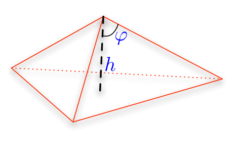
Just like the 1-dimensional case, Algorithm 2 proceeds in epochs. We start with the optimization domain $\mathcal{X}$ , and at the beginning we set $\mathcal{X}_{0}=\mathcal{X}$ . At the beginning of epoch $\tau$ , we have a current feasible set $\mathcal{X}_{\tau}$ which contains an approximate optimum of the convex function. The epoch ends with discarding some portion of the set $\mathcal{X}_{\tau}$ in such a way that we still retain at least one approximate optimum in the remaining set $\mathcal{X}_{\tau+1}$ .

At the start of the epoch $\tau$ , we apply an affine transformation to $\mathcal{X}_{\tau}$ so that the smallest volume ellipsoid containing it is a Euclidean ball of radius $R_{\tau}$ (denoted as $\mathcal{B}(R_{\tau}))$ . We define $r_{\tau}=R_{\tau}/c_{1}d$ for a constant $c_{1}\geq 1$ , so that $\mathcal{B}(r_{\tau})\subseteq\mathcal{X}_{\tau}$ (such a construction is always possible, see, e.g., Lecture 1, p. 2 [4]). We will use the notation $\mathcal{B}_{\tau}$ to refer to the enclosing ball. Within each epoch, the algorithm proceeds in several rounds, each round maintaining a value $\gamma_{i}$ which is successively halved.

Let $x_{0}$ be the center of the ball $\mathbb{B}(R_{\tau})$ containing $\mathcal{X}_{\tau}$ . At the start of a round $i$ , we construct a regular simplex centered at $x_{0}$ and contained in $\mathbb{B}(r_{\tau})$ . The algorithm queries the function $f$ at all the vertices of the simplex, denoted by $x_{1}.\dots,x_{d+1}$ , until the CI’s at each vertex shrink to $\gamma_{i}$ . The algorithm then picks the point $y_{1}$ for which the average of observed function values is the largest. By construction, we are guaranteed that $f(y_{1})\geq f(x_{j})-\gamma_{i}$ for all $j=1,\dots,d+1$ . This step is depicted in Figure 5.

The algorithm now successively constructs a sequence of pyramids, with the goal of identifying a region of the feasible set $\mathcal{X}_{\tau}$ such that at least one approximate optimum of $f$ lies outside the selected region. This region will be discarded at the end of the epoch. The construction of the pyramids follows the construction from Section 9.2.2 of the book [15]. The pyramids we construct will have an angle $2\varphi$ at the apex, where $\cos\varphi=c_{2}/d$ . The base of the pyramid consists of vertices $z_{1},\dots,z_{d}$ such that $z_{i}-x_{0}$ and $y_{1}-z_{i}$ are orthogonal. We note that the construction of such a pyramid is always possible—we take a sphere with $y_{1}-x_{0}$ as the diameter, and arrange $z_{1},\dots,z_{d}$ on the boundary of the sphere such that the angle between $y_{1}-x_{0}$ and $y_{1}-z_{i}$ is $\varphi$ . The construction of the pyramid is depicted in Figure 6. Given this pyramid, we set ${\widehat{\gamma}}=1$ , and sample the function at $y_{1}$ and $z_{1},\dots,z_{d}$ as well as the center of the pyramid until the CI’s all shrink to ${\widehat{\gamma}}$ . Let top and bottom denote the vertices of the pyramid (including $y_{1}$ ) with the largest and the smallest function value estimates resp. For consistency, we will also use apex to denote the apex $y_{1}$ . We then check for one of the following conditions:

1.

If $\operatorname{LB}_{\widehat{\gamma}}(\mbox{{top}})\geq\operatorname{UB}_{\widehat{\gamma}}(\mbox{{bottom}})+\Delta_{\tau}({\widehat{\gamma}})$ , we proceed based on the separation between top and apex CI’s as illustrated in Figures 7(a) and 7(b).

(a) (b)

Figure 7: Relative ordering of confidence intervals of top, bottom and apex in cases 1(a) and 1(b) of the algorithm resp.
1. (a)
  
  If $\operatorname{LB}_{\widehat{\gamma}}(\mbox{{top}})\geq\operatorname{UB}_{\widehat{\gamma}}(\mbox{{apex}})+{\widehat{\gamma}}$ , then we know that with high probability
  
  $f(\mbox{{top}})\geq f(\mbox{{apex}})+{\widehat{\gamma}}\geq f(\mbox{{apex}})+\gamma_{i}.$ (2)
  
  In this case, we set top to be the apex of the next pyramid, reset ${\widehat{\gamma}}=1$ and continue the sampling procedure on the next pyramid.
2. (b)
  
  If $\operatorname{LB}_{\widehat{\gamma}}(\mbox{{top}})\leq\operatorname{UB}_{\widehat{\gamma}}(\mbox{{apex}})+{\widehat{\gamma}}$ , then we know that $\operatorname{LB}_{\widehat{\gamma}}(\mbox{{apex}})\geq\operatorname{UB}_{\widehat{\gamma}}(\mbox{{bottom}})+\Delta_{\tau}({\widehat{\gamma}})-2{\widehat{\gamma}}$ . In this case, we declare the epoch over and pass the current apex to the cone-cutting step.
2.

If $\operatorname{LB}_{\widehat{\gamma}}(\mbox{{top}})\leq\operatorname{UB}_{\widehat{\gamma}}(\mbox{{bottom}})+\Delta_{\tau}({\widehat{\gamma}})$ , then one of the two events depicted in Figures 8(a) or 8(b) has to happen:

(a) (b)

Figure 8: Relative ordering of confidence intervals of top, bottom and center $\operatorname{\textsc{center}}$ in cases 2(a) and 2(b) of the algorithm resp.
1. (a)
  
  If $\operatorname{UB}_{\widehat{\gamma}}(\operatorname{\textsc{center}})\geq\operatorname{LB}_{\widehat{\gamma}}(\mbox{{bottom}})-\bar{\Delta}_{\tau}({\widehat{\gamma}})$ , then all of the vertices and the center of the pyramid have their function values within a $2\Delta_{\tau}({\widehat{\gamma}})+3{\widehat{\gamma}}$ interval. In this case, we set ${\widehat{\gamma}}={\widehat{\gamma}}/2$ . If this sets ${\widehat{\gamma}}<\gamma_{i}$ , we start the next round with $\gamma_{i+1}=\gamma_{i}/2$ . Otherwise, we continue sampling the current pyramid with the new value of ${\widehat{\gamma}}$ .
2. (b)
  
  If $\operatorname{UB}_{\widehat{\gamma}}(\operatorname{\textsc{center}})\leq\operatorname{LB}_{\widehat{\gamma}}(\mbox{{bottom}})-\bar{\Delta}_{\tau}({\widehat{\gamma}})$ , then we terminate the epoch and pass the center and the current apex to the hat-raising step.

Hat-Raising:

This step happens when we construct a pyramid where $\operatorname{LB}_{\widehat{\gamma}}(\mbox{{top}})\leq\operatorname{UB}_{\widehat{\gamma}}(\mbox{{bottom}})+\Delta_{\tau}({\widehat{\gamma}})$ but $\operatorname{UB}_{\widehat{\gamma}}(\operatorname{\textsc{center}})\leq\operatorname{LB}_{\widehat{\gamma}}(\mbox{{bottom}})-\bar{\Delta}_{\tau}({\widehat{\gamma}})$ (see Fig. 8(b) for an illustration). In this case, we will show that if we move the apex of the pyramid a little from $y_{i}$ to $y^{{}^{\prime}}_{i}$ , then $y^{{}^{\prime}}_{i}$ ’s CI is above the top CI while the angle of the new pyramid at $y^{{}^{\prime}}_{i}$ is not much smaller than $2\varphi$ . In particular, letting $\operatorname{\textsc{center}}_{i}$ denote the center of the pyramid, we set $y^{{}^{\prime}}_{i}=y_{i}+(y_{i}-\operatorname{\textsc{center}}_{i})$ . Figure 9 shows transformation of the pyramid involved in this step. The correctness of this step and the sufficiency of the perturbation from $y$ to $y^{{}^{\prime}}$ will be proved in the next section.

Cone-cutting:

This step is the concluding step for an epoch. The algorithm gets to this step either through case 1(b) or through the hat-raising step. In either case, we have a pyramid with an apex $y$ , base $z_{1},\dots,z_{d}$ and an angle $2\bar{\varphi}$ at the apex, where $\cos(\bar{\varphi})\leq 1/2d$ . We now define a cone

\mathcal{K}_{\tau}=\{x~|~\exists\lambda>0,\alpha_{1},\dots,\alpha_{d}>0,\sum_{i=1}^{d}\alpha_{i}=1~:~x=y-\lambda\sum_{i=1}^{d}\alpha_{i}(z_{i}-y)\}

(3)

which is centered at $y$ and a reflection of the pyramid around the apex. By construction, the cone $\mathcal{K}_{\tau}$ has an angle $2\bar{\varphi}$ at its apex. We set $\mathcal{B}_{\tau+1}^{{}^{\prime}}$ to be the ellipsoid of minimum volume containing $\mathcal{B}_{\tau}\setminus\mathcal{K}_{\tau}$ and define $\mathcal{X}_{\tau+1}=\mathcal{X}_{\tau}\cap\mathcal{B}_{\tau+1}^{{}^{\prime}}$ . This is illustrated in Figure 10. Finally, we put things back into an isotropic position and $\mathcal{B}_{\tau+1}$ is the ball containing $\mathcal{X}_{\tau+1}$ is in the isotropic coordinates, which is just obtained by applying an affine transformation to $\mathcal{B}_{\tau+1}^{{}^{\prime}}$ .

Let us end the description with a brief discussion regarding the computational aspects of this algorithm. It is clear that the most computationally intensive steps of this algorithm are the cone-cutting and isotropic transformation at the end. However, these steps are exactly analogous to an implementation of the classical ellipsoid method. In particular, the equation for $\mathcal{B}^{{}^{\prime}}_{\tau+1}$ is known in closed form [11]. Furthermore, the affine transformations needed to the reshape the set can be computed via rank-one matrix updates and hence computation of inverses can be done efficiently as well (see e.g. [11] for the relevant implementation details of the ellipsoid method).

6 Analysis

We start by showing the correctness of the algorithm and then proceed to regret analysis. To avoid having probabilities throughout our analysis, we define an event $\mathcal{E}$ where at each epoch $\tau$ , and each round $i$ , $f(x)\in[\operatorname{LB}_{\gamma_{i}}(x),\operatorname{UB}_{\gamma_{i}}(x)]$ for any point $x$ sampled in the round. We will carry out the remainder of the analysis conditioned on $\mathcal{E}$ and bound the probability of $\mathcal{E}^{c}$ at the end. We also assume that the algorithm is run with the settings

\Delta_{\tau}(\gamma)=\left(\frac{6c_{1}d^{4}}{c_{2}^{2}}+3\right)\gamma\quad\mbox{and}\quad\bar{\Delta}_{\tau}(\gamma)=\left(\frac{6c_{1}d^{4}}{c_{2}^{2}}+5\right)\gamma,

(4)

and constants $c_{1}\geq 64$ , $c_{2}\leq 32$ .

6.1 Correctness of the algorithm

In order to complete the proof of our algorithm’s correctness, we only need to further show that when the algorithm proceeds to cone-cutting via case 1(b), then it does not discard all the approximate optima of $f$ by mistake, and show that the hat-raising step is indeed correct as claimed. These two claims are established in the next couple of lemmas.

For these two lemmas, we assume that the distance of the apex of any $\Pi$ constructed in epoch $\tau$ from the center of $\mathbb{B}(r_{\tau})$ is at least $r_{\tau}/d$ . This assumption will be established later.

Lemma 5.

Let $\mathcal{K}_{\tau}$ be the cone discarded at epoch $\tau$ which is ended through Case (1b) in round $i$ . Let bottom be the lowest CI of the last pyramid $\Pi$ constructed in the epoch, and assume the distance from the apex of $\Pi$ to the center of $\mathbb{B}(r_{\tau})$ is at least $r_{\tau}/d$ . Then $f(x)\geq f(\mbox{{bottom}})+\gamma_{i}$ for all $x\in\mathcal{K}_{\tau}$ .

Proof.

Consider any $x\in\mathcal{K}_{\tau}$ . By construction, there is a point $z$ in the base of the pyramid $\Pi$ such that the apex $y$ of $\Pi$ satisfies $y=\alpha z+(1-\alpha)x$ for some $\alpha\in[0,1)$ (see Fig. 11 for a graphical illustration).

Since $f$ is convex and $z$ is in the base of the pyramid, we have that

f(z)\leq f(\mbox{{top}})\leq f(y)+3{\widehat{\gamma}}

. Also, the condition of Case (1b) ensures

f(y)>f(\mbox{{bottom}})+\Delta_{\tau}({\widehat{\gamma}})-2{\widehat{\gamma}}

where ${\widehat{\gamma}}$ is the CI level used for the pyramid. Then by convexity of $f$

\displaystyle f(y)\leq\alpha f(z)+(1-\alpha)f(x)\leq\alpha(f(y)+3{\widehat{\gamma}})+(1-\alpha)f(x).

Simplifying yields

f(x)\geq f(y)-3\frac{\alpha}{1-\alpha}{\widehat{\gamma}}>f(\mbox{{bottom}})+\Delta_{\tau}({\widehat{\gamma}})-2{\widehat{\gamma}}-3\frac{\alpha}{1-\alpha}{\widehat{\gamma}}.

Also, we know that $\alpha/(1-\alpha)=\|y-x\|/\|y-z\|$ . Because $x\in\mathbb{B}(R_{\tau})$ , $\|y-x\|\leq 2R_{\tau}\leq 2c_{1}dr_{\tau}$ . Moreover, $\|y-z\|$ is at least the height of $\Pi$ , which is at least $r_{\tau}c_{2}^{2}/d^{3}$ by Lemma 15. Therefore

\frac{\alpha}{1-\alpha}=\frac{\|y-x\|}{\|y-z\|}\leq\frac{2c_{1}dr_{\tau}}{r_{\tau}c_{2}^{2}/d^{3}}\leq\frac{2c_{1}d^{4}}{c_{2}^{2}}.

Thus, we have

\displaystyle f(x)

\displaystyle>f(\mbox{{bottom}})+\Delta_{\tau}({\widehat{\gamma}})-2{\widehat{\gamma}}-\frac{6c_{1}d^{4}}{c_{2}^{2}}{\widehat{\gamma}}\geq f(\mbox{{bottom}})+\gamma_{i},

(5)

where the last line uses the setting of $\Delta_{\tau}({\widehat{\gamma}})$ (4), completing the proof of the lemma. ∎

This lemma guarantees that we cannot discard all the approximate minima of $f$ by mistake in case 1(b), and that any point discarded by the algorithm through this step in round $i$ has regret at least $\gamma_{i}$ . The final check that needs to be done is the correctness of the hat-raising step which we do in the next lemma.

Lemma 6.

Let $\Pi^{\prime}$ be the new pyramid formed in hat-raising with apex $y^{\prime}$ and same base as $\Pi$ in round $i$ of epoch $\tau$ , and let $\mathcal{K}_{\tau}^{\prime}$ be the cone discarded. Assume the distance from the apex of $\Pi$ to the center of $\mathbb{B}(r_{\tau})$ is at least $r_{\tau}/d$ . Then the $\Pi^{\prime}$ has an angle $\bar{\varphi}$ at the apex with $\cos\bar{\varphi}\leq 2c_{2}/d$ , height at most $2r_{\tau}c_{1}^{2}/d^{2}$ , and with every point $x$ in the cone $\mathcal{K}_{\tau}^{\prime}$ having $f(x)\geq f(x^{*})+\gamma_{i}$ .

Proof.

Let $y^{\prime}:=y+(y-\operatorname{\textsc{center}})$ be the apex of $\Pi^{\prime}$ . Let $h$ be the height of $\Pi$ (the distance from $y$ to the base), $h^{\prime}$ be the height of $\Pi^{\prime}$ , and $b$ be the distance from any vertex of the base to the center of the base. Then $h^{\prime}<2h\leq 2r_{\tau}c_{1}^{2}/d^{2}$ by Lemma 15. Moreover, since $\cos(\varphi)=h/\sqrt{h^{2}+b^{2}}=1/d$ , we have $\cos(\bar{\varphi})=h^{\prime}/\sqrt{{h^{\prime}}^{2}+b^{2}}\leq 2h/\sqrt{h^{2}+b^{2}}=2\cos(\varphi)=2c_{2}/d$ .

It remains to show that every $x\in\mathcal{K}_{\tau}^{\prime}$ has $f(x)\geq f(x^{*})+{\widehat{\gamma}}$ . By convexity of $f$ , $f(y)\leq(f(y^{\prime})+f(\operatorname{\textsc{center}}))/2$ , so $f(y^{\prime})\geq 2f(y)-f(\operatorname{\textsc{center}})$ . Since we enter hat-raising via case 2(b) of the algorithm, we know that $f(\operatorname{\textsc{center}})\leq f(y)-\bar{\Delta}_{\tau}({\widehat{\gamma}})$ , so

f(y^{\prime})\geq f(y)+\bar{\Delta}_{\tau}({\widehat{\gamma}}).

The condition for entering case 2(b) also implies that $f(y)>f(\mbox{{top}})-\Delta_{\tau}({\widehat{\gamma}})-2{\widehat{\gamma}}>f(x)-\Delta_{\tau}({\widehat{\gamma}})-2{\widehat{\gamma}}$ for all $x\in\Pi$ , and therefore for any $z$ on the base of $\Pi$ ,

f(y^{\prime})>f(z)+\bar{\Delta}_{\tau}({\widehat{\gamma}})-\Delta_{\tau}({\widehat{\gamma}})-2{\widehat{\gamma}}\geq f(z),

where the last line uses the settings of $\Delta_{\tau}({\widehat{\gamma}})$ and $\bar{\Delta}_{\tau}({\widehat{\gamma}})$ (4). Now take any $x\in\mathcal{K}_{\tau}^{\prime}$ . There exists $\alpha\in[0,1)$ and $z$ on the base of $\Pi^{\prime}$ such that $y^{\prime}=\alpha z+(1-\alpha)x$ , so by convexity of $f$ , $f(y^{\prime})\leq\alpha f(z)+(1-\alpha)f(x)\leq\alpha f(y^{\prime})+(1-\alpha)f(x)$ , which implies $f(x)\geq f(y^{\prime})\geq f(y)+\bar{\Delta}_{\tau}({\widehat{\gamma}})\geq f(x^{*})+\gamma_{i}$ . ∎

6.2 Regret analysis

The following theorem states our regret guarantee on the performance of the algorithm 2.

Theorem 2.

Suppose Algorithm 2 is run with $c_{1}\geq 64$ , $c_{2}\leq 1/32$ and parameters

\Delta_{\tau}(\gamma)=\left(\frac{6c_{1}d^{4}}{c_{2}^{2}}+3\right)\gamma\quad\mbox{and}\quad\bar{\Delta}_{\tau}(\gamma)=\left(\frac{6c_{1}d^{4}}{c_{2}^{2}}+5\right)\gamma.

Then with probability at least $1-1/T$ , the net regret incurred by the algorithm is bounded by

768d^{3}\sigma\sqrt{T}\log^{2}T\left(\frac{2d^{2}\log d}{c_{2}^{2}}+1\right)\left(\frac{4d^{7}c_{1}}{c_{2}^{3}}+\frac{d(d+1)}{c_{2}}\right)\left(\frac{4c_{1}d^{4}}{c_{2}^{2}}+11\right).

Remarks:

The prior knowledge of $T$ in Algorithm 2 and Theorem 2 can again be addressed using a doubling argument. As earlier, Theorem 2 is optimal in the dependence on $T$ . The large dependence on $d$ is also seen in Nemirovski and Yudin [15] who obtain a $d^{7}$ scaling in noiseless case and leave it an unspecified polynomial in the noisy case. Using random walk ideas [5] to improve the dependence on $d$ is an interesting question for future research.

The analysis will start by controlling the regret incurred on different rounds, and then we will piece it together across rounds and epochs to get the net regret for the entire procedure.

6.2.1 Bounding the regret incurred in one round

We will start by a simple lemma regarding the regret incurred while playing a pyramid if the condition 2(a) is encountered in the algorithm. This lemma highlights the importance of evaluating the function at the center of the pyramid, a step that was not needed in the framework of Nemirovski and Yudin [15]. We will use the symbol $\Pi$ to refer to a generic pyramid constructed by the algorithm during the course of its operation, with apex $y$ , base $z_{1},\dots,z_{d}$ , center $\operatorname{\textsc{center}}$ and with an angle $\varphi$ at the apex. We also recall that the pyramids constructed by the algorithm are such that the distance from the center to the base is at least $r_{\tau}c_{2}^{2}/d^{3}$ .

Lemma 7.

Suppose the algorithm reaches case 2(a) in round $i$ of epoch $\tau$ , and assume $x^{*}\in\mathbb{B}(R_{\tau})$ where $x^{*}$ is the minimizer of $f$ . Let $\Pi$ be the current pyramid and ${\widehat{\gamma}}$ be the current CI width. Assume the distance from the apex of $\Pi$ to the center of $\mathbb{B}(r_{\tau})$ is at least $r_{\tau}/d$ . Then the net regret incurred while evaluating the function on $\Pi$ in round $i$ is at most

\frac{6d\sigma\log T}{{\widehat{\gamma}}}\left(\frac{4d^{7}c_{1}}{c_{2}^{3}}+\frac{d(d+2)}{c_{2}}\right)\left(\frac{12c_{1}d^{4}}{c_{2}^{2}}+11\right).

Proof.

The proof is a consequence of convexity. We start by bounding the variation of the function inside the pyramid. Since the pyramid is a convex hull of its vertices, we know that the function value at any point in the pyramid is also upper bounded by the largest function value achieved at any vertex. Furthermore, the condition for reaching Case (2a) implies that the function value at any vertex is at most $f(\operatorname{\textsc{center}})+\Delta_{\tau}({\widehat{\gamma}})+\bar{\Delta}_{\tau}({\widehat{\gamma}})+3{\widehat{\gamma}}$ , and therefore

f(x)\leq f(\operatorname{\textsc{center}})+\Delta_{\tau}({\widehat{\gamma}})+\bar{\Delta}_{\tau}({\widehat{\gamma}})+3{\widehat{\gamma}}\quad\text{for all $x\in\Pi$.}

(6)

For brevity, we use the shorthand $\delta:=\Delta_{\tau}({\widehat{\gamma}})+\bar{\Delta}_{\tau}({\widehat{\gamma}})+3{\widehat{\gamma}}$ . Consider any point $x\in\Pi$ , and let $b$ be the point where the ray $\operatorname{\textsc{center}}-x$ intersects a face of $\Pi$ on the other side. Then we know that there is a positive constant $\alpha\in[0,1]$ such that $\operatorname{\textsc{center}}=\alpha x+(1-\alpha)b$ ; in particular, $(1-\alpha)/\alpha=\|\operatorname{\textsc{center}}-x\|/\|\operatorname{\textsc{center}}-b\|$ . Note that $\|\operatorname{\textsc{center}}-x\|$ is at most the distance from $\operatorname{\textsc{center}}$ to a vertex of $\Pi$ , and $\|\operatorname{\textsc{center}}-b\|$ is at least the radius of the largest ball centered at $\operatorname{\textsc{center}}$ inscribed in $\Pi$ . Therefore by Lemma 16(b),

\frac{1-\alpha}{\alpha}=\frac{\|\operatorname{\textsc{center}}-x\|}{\|\operatorname{\textsc{center}}-b\|}\leq\frac{d(d+1)}{c_{2}}.

Then the convexity of $f$ and the upper bound on function values over $\Pi$ from (6) guarantee that

f(\operatorname{\textsc{center}})\leq\alpha f(x)+(1-\alpha)f(b)\leq\alpha f(x)+(1-\alpha)(f(\operatorname{\textsc{center}})+\delta).

Rearranging, we get

\displaystyle f(x)\geq f(\operatorname{\textsc{center}})-\frac{d(d+1)\delta}{c_{2}}.

(7)

Combining equations (6) and (7) we have shown that for any $x,x^{\prime}\in\Pi$

|f(x)-f(x^{\prime})|\leq\frac{d(d+2)\delta}{c_{2}}.

(8)

Now we will bootstrap to show that the above bound implies low regret while sampling the vertices and center of $\Pi$ . We first note that if $x^{*}\in\Pi$ , then the regret on any vertex or the center is bounded by $d(d+2)\delta/c_{2}$ . In that case, the regret incurred by sampling the vertices and center of this pyramid (so $d+2$ points) is bounded by $(d+2)\cdot d(d+2)\delta/c_{2}$ . Furthermore, we only need to sample each point pyramid $2\sigma\log T/{{\widehat{\gamma}}}^{2}$ times to get the CI’s of width ${\widehat{\gamma}}$ , which completes the proof in this case, so the total regret incurred is

(d+2)\frac{d(d+2)\delta}{c_{2}}\cdot\frac{2\sigma\log T}{{\widehat{\gamma}}^{2}}.

Now we consider the case where $x^{*}\notin\Pi$ . Recall that Lemma 5 guarantees that $x^{*}\in\mathcal{B}_{\tau}$ . There is a point $b$ on a face of $\Pi$ such that $b=\alpha x^{*}+(1-\alpha)\operatorname{\textsc{center}}$ for some $\alpha\in[0,1]$ . Then $\alpha=\|\operatorname{\textsc{center}}-b\|/\|\operatorname{\textsc{center}}-x^{*}\|$ . By the triangle inequality, $\|\operatorname{\textsc{center}}-x^{*}\|\leq 2R_{\tau}=2c_{1}dr_{\tau}$ . Moreover, $\|\operatorname{\textsc{center}}-b\|$ is at least the radius of the largest ball centered at $\operatorname{\textsc{center}}$ inscribed in $\Pi$ , which is at least $r_{\tau}c_{2}^{2}/(2d^{4})$ by Lemma 16. Therefore $\alpha\geq c_{2}^{2}/(4c_{1}d^{5})$ . By convexity and Equation (7),

f(\operatorname{\textsc{center}})-\frac{d(d+2)\delta}{c_{2}}\leq f(b)\leq\alpha f(x^{*})+(1-\alpha)f(\operatorname{\textsc{center}}),

f(x^{*})\geq f(\operatorname{\textsc{center}})-\frac{d(d+2)\delta}{c_{2}\alpha}\geq f(\operatorname{\textsc{center}})-\frac{4d^{7}c_{1}\delta}{c_{2}^{3}}\geq f(x)-\frac{4d^{7}c_{1}\delta}{c_{2}^{3}}-\frac{d(d+2)\delta}{c_{2}}

for any $x\in\Pi$ . Therefore, using the same argument as before, the net regret incurred in the round is

(d+2)\left(\frac{4d^{7}c_{1}}{c_{2}^{3}}+\frac{d(d+2)}{c_{2}}\right)\delta\cdot\frac{2\sigma\log T}{{\widehat{\gamma}}^{2}}.

Substituting in the values of $\Delta_{\tau}({\widehat{\gamma}})$ and $\bar{\Delta}_{\tau}({\widehat{\gamma}})$ completes the proof. ∎

Lemma 7 is critical because it allows us to claim that at any round, when we sample the function over a pyramid with a value ${\widehat{\gamma}}$ , then the regret on that pyramid during this sampling is at most $\poly(d)/{\widehat{\gamma}}$ since we must have been in case 2(a) with $2{\widehat{\gamma}}$ if we’re using ${\widehat{\gamma}}$ . The only exception is at first round, where this statement holds trivially as the function is 1-Lipschitz by assumption.

We next show that the algorithm can visit the case 1(a) only a bounded number of times every round. The round is ended when the algorithm enters cases 1(b) or 2(b), and the regret incurred on case 2(a) would be bounded using the above Lemma 7.

The key idea for this bound is present in Section 9.2.2 of Nemirovski and Yudin [15]. We need a slight modification of their argument due to the fact that the function evaluations have noise and our sampling strategy is a little different from theirs.

Lemma 8.

At any round, the number of visits to case 1(a) is $2d^{2}\log d/c_{2}^{2}$ , and each pyramid $\Pi$ constructed by the algorithm satisfies $\|y-x_{0}\|\geq r_{\tau}/d$ , where $y$ is the apex of $\Pi$ .

Proof.

The proof follows by a simple geometric argument that exploits the fact that we have an angle $2\varphi$ at the apex of our pyramid which is almost equal to $\pi$ , and that $y-x_{0}$ and $z_{i}-x_{0}$ are orthogonal for any pyramid $\Pi$ we construct (see Figure 6). By definition of case 1(a), $\mbox{{top}}\neq y$ , so we assume $\mbox{{top}}=z_{1}$ wlog. By construction,

\|z_{1}-x_{0}\|=\sin\varphi\|y-x_{0}\|.

(9)

Since this step applies every time we enter case 1(a), the total number $k$ of visits to case 1(a) satisfies

\|z_{1}-x_{0}\|=(\sin\varphi)^{k}r_{\tau},

where we recall that $r_{\tau}$ is the radius of the regular simplex we construct in the first step on every round. We further note that for a regular simplex of radius $r_{\tau}$ , a Euclidean ball of radius $r_{\tau}/d$ is contained in the simplex. We also note that by construction, $\cos\varphi=c_{2}/d$ and hence $\sin\varphi=\sqrt{1-c_{2}^{2}/d^{2}}\leq 1-c_{2}^{2}/(2d^{2})$ . Hence, setting $k=2d^{2}\log d/c_{2}^{2}$ suffices to ensure that $\|z_{1}-x_{0}\|\leq r_{\tau}/d$ guaranteeing that $z_{1}$ lies in the initial simplex of radius $r_{\tau}$ centered at $x_{0}$ , as depicted in Figure 12.

Let $y_{1},\dots,y_{k}$ be the apexes of the pyramids we have constructed in this round. Then by construction, we have a sequence of points such that

f(z_{1})=f(\mbox{{top}})\geq f(y_{k})+\gamma\geq f(y_{k-1})+2\gamma\dots\geq f(y_{1})+k\gamma.

On the other hand, we know that $y_{1}$ satisfies $f(y_{1})\geq f(x_{i})-\gamma$ for all the vertices $x_{i}$ of the simplex by definition of $y_{1}$ . Since $z_{1}$ lies in the simplex, convexity of $f$ guarantees that

f(y_{1})\geq f(z_{1})-\gamma\geq f(y_{1})+(k-1)\gamma,

which is a contradiction unless $k\leq 1$ . Thus it must be the case that $z_{1}$ is not in the simplex if $k>1$ , in which case $k$ can be at most $2d^{2}\log d/c_{2}^{2}$ . ∎

This lemma guarantees that in at most $2d^{2}\log d/c_{2}^{2}$ pyramid constructions, the algorithm will enter one of cases 1(b) or 2(b) and terminate the epoch, unless the CI level $\gamma$ at this round is insufficient to resolve things and we end in case 2(a). It also shows that all the pyramids constructed by our algorithm are sufficiently far from the center which is assumed by Lemmas 5- 7. Until now, we have focused on controlling the regret on the pyramids we construct, which is convenient since we sample the center points of the pyramids. To bound the regret incurred over one round, we also need to control the regret over the initial simplex we query at every round. We start with a lemma that shows how to control the net regret accrued over an entire round, when the round ends in case 2(a).

Lemma 9.

For any round with a CI width of $\gamma$ that terminates in case 2(a), the net regret incurred on the round is at most

\frac{24d\sigma\log T}{\gamma}\left(\frac{2d^{2}\log d}{c_{2}^{2}}+1\right)\left(\frac{4d^{7}c_{1}}{c_{2}^{3}}+\frac{d(d+2)}{c_{2}}\right)\left(\frac{12c_{1}d^{4}}{c_{2}^{2}}+11\right)

Proof.

Suppose we constructed a total of $k$ pyramids on the round, with $k\leq 2d^{2}\log d/c_{2}$ by Lemma 8. Then we know that the instantaneous regret on any point of the $k_{th}$ pyramid $\Pi_{k}$ is bounded by

\delta:=\gamma\left(\frac{4d^{7}c_{1}}{c_{2}^{3}}+\frac{d(d+2)}{c_{2}}\right)\left(\frac{12c_{1}d^{4}}{c_{2}^{2}}+11\right),

by Lemma 7. We also note that by construction, $y_{k}$ is the top vertex of the $(k-1)$ st pyramid $\Pi_{k-1}$ . Hence by definition of case 1(a) (which caused us to go from $\Pi_{k-1}$ to $\Pi_{k}$ ), we know that $f(x)\leq f(y_{k})+\gamma$ for all $x\in\Pi_{k-1}$ . Reasoning in the same way, we get that the function value at each vertex of the pyramid we constructed in this round is bounded by the function value at $y_{k}$ . Furthermore, just like the proof of Lemma 8, the function value at any vertex of the initial simplex is also bounded by the function value at $y_{k}$ . As a result, the instantaneous regret incurred at any point we sampled in this round is bounded by the net regret at $y_{k}$ which is at most by $\delta$ using Lemma 7. Since every pyramid as well as the simplex samples at most $d+2$ vertices, and the total number of pyramids we construct is bounded by Lemma 8, we query at most $(d+2)(2d^{2}/c_{2}^{2}\log d+1)$ points at any round. In order to bound the number of queries made at any point, we observe that for a CI level ${\widehat{\gamma}}$ , we make $2\sigma\log T/{\widehat{\gamma}}^{2}$ queries. Suppose $\gamma=2^{-1}$ . Since ${\widehat{\gamma}}$ is geometrically decreased to $\gamma$ , the total number of queries made at any point is bounded by

\displaystyle\sum_{j=1}^{i}\frac{2\sigma\log T}{2^{-2j}}\leq 8\sigma\log T2^{2i}=\frac{8\sigma\log T}{\gamma^{2}}.

Putting all the pieces together, the net regret accrued over this round is at most

\frac{24d\sigma\log T}{\gamma}\left(\frac{2d^{2}\log d}{c_{2}^{2}}+1\right)\left(\frac{4d^{7}c_{1}}{c_{2}^{3}}+\frac{d(d+2)}{c_{2}}\right)\left(\frac{12c_{1}d^{4}}{c_{2}^{2}}+11\right),

which completes the proof. ∎

We are now in a position to state a regret bound on the net regret incurred in any round. The key idea would be to use the bound from Lemma 9 to bound the regret even when the algorithm terminates in cases 1(b) or 2(b).

Lemma 10.

For any round that terminates in a CI level $\gamma$ , the net regret over the round is bounded by

\frac{48d\sigma\log T}{\gamma}\left(\frac{2d^{2}\log d}{c_{2}^{2}}+1\right)\left(\frac{4d^{7}c_{1}}{c_{2}^{3}}+\frac{d(d+2)}{c_{2}}\right)\left(\frac{12c_{1}d^{4}}{c_{2}^{2}}+11\right).

Proof.

We just need to control the regret incurred in rounds that end in cases 1(b) or 2(b). We recall from the description of the algorithm that a CI level of $\gamma$ is used at a round only when the algorithm terminates the round with a CI level of $2\gamma$ in case 2(a). The only exception is the first round with $\gamma=1$ , where the instantaneous regret is bounded by 1 at any point using the Lipschitz assumption. Now suppose we did end a round with CI level $2\gamma$ in case 2(a). In particular, the proof of Lemma 9 guarantees that the instantaneous regret at any vertex of the simplex we construct is at most

2\gamma\left(\frac{4d^{7}c_{1}}{c_{2}^{3}}+\frac{d(d+2)}{c_{2}}\right)\left(\frac{12c_{1}d^{4}}{c_{2}^{2}}+11\right)

Now consider any pyramid constructed on this round. We know that the instantaneous regret incurred if the pyramid ends in case 2(a) is bounded by Lemma 7. Furthermore, if the algorithm was in cases 1(a), 1(b) or 2(b) with a CI level ${\widehat{\gamma}}$ (which could be larger than $\gamma$ in general), then it must have been in case 2(a) with a CI level $2{\widehat{\gamma}}$ . Hence the instantaneous regret on the vertices of the pyramid is at most

2{\widehat{\gamma}}\left(\frac{4d^{7}c_{1}}{c_{2}^{3}}+\frac{d(d+2)}{c_{2}}\right)\left(\frac{12c_{1}d^{4}}{c_{2}^{2}}+11\right),

and we make at most $\frac{8\sigma\log T}{{\widehat{\gamma}}^{2}}$ queries on any point of the pyramid by a similar argument like the previous lemma. Thus the net regret incurred at any pyramid constructed by the algorithm is at most

\frac{48d\sigma\log T}{{\widehat{\gamma}}}\left(\frac{4d^{7}c_{1}}{c_{2}^{3}}+\frac{d(d+2)}{c_{2}}\right)\left(\frac{12c_{1}d^{4}}{c_{2}^{2}}+11\right),

Recalling our bound on the number of pyramids constructed at any round completes the proof. ∎

Putting all the pieces together, we have shown that the regret incurred on any round with a CI level $\gamma$ is bounded by $C/\gamma$ , where $C$ comes from the above lemmas. We further observe that since $\gamma$ is reduced geometrically, the net regret incurred on an epoch where the largest CI level we encounter is $\gamma$ is at most

\sum_{j=1}^{i}\frac{C}{2^{-j}}\leq 2C2^{i}=2C/\gamma.

This allows us to get a bound on the regret of one epoch stated in the next lemma.

Lemma 11.

The regret in any epoch which ends in CI level $\gamma$ is at most

\frac{96d\sigma\log T}{\gamma}\left(\frac{2d^{2}\log d}{c_{2}^{2}}+1\right)\left(\frac{4d^{7}c_{1}}{c_{2}^{3}}+\frac{d(d+2)}{c_{2}}\right)\left(\frac{12c_{1}d^{4}}{c_{2}^{2}}+11\right).

(10)

6.2.2 Bound on the number of epochs

In order to bound the number of epochs, we first need to show that the cone-cutting step discards a sizeable chunk of the set $\mathcal{X}_{\tau}$ in epoch $\tau$ . Recall that we need to understand the ratio of the volumes of $\mathcal{B}_{\tau+1}$ to $\mathcal{B}_{\tau}$ in order to understand the amount of volume discarded in any epoch.

Lemma 12.

Let $\mathcal{B}_{\tau}$ be the smallest ball containing $\mathcal{X}_{\tau}$ , and let $\mathcal{B}^{{}^{\prime}}_{\tau+1}$ be the minimum volume ellipsoid containing $\mathcal{B}_{\tau}\setminus\mathcal{K}_{\tau}$ . Then for small enough constants $c_{1},c_{2}$ , $\mbox{vol}(\mathcal{B}^{{}^{\prime}}_{\tau+1})\leq\rho\cdot\mbox{vol}(\mathcal{B}_{\tau})$ for $\rho=\exp(-\frac{1}{4(d+1)})$ .

Proof.

This lemma is analogous to the volume reduction results proved in the analysis of ellipsoid method for convex programming with a gradient oracle. We start by arguing that it suffices to consider the intersection of $\mathcal{B}_{\tau}$ with a half-space in order to understand the set $\mathcal{B}_{\tau}\setminus\mathcal{K}_{\tau}$ . It is clear from the figure that we only increase the volume of the enclosing ellipsoid $\mathcal{B}^{{}^{\prime}}_{\tau+1}$ if we consider discarding only the spherical cap instead of discarding the entire cone. But the spherical cap is exactly obtained by taking the intersection of $\mathcal{B}_{\tau}$ with a half-space.

The choices of the constants $c_{1},c_{2}$ earlier guarantee that the distance of the hyperplane from the origin is at most $R_{\tau}/(4(d+1))$ . This is because the apex of the cone $\mathcal{K}_{\tau}$ is always contained in $\mathbb{B}(r_{\tau})$ by construction and the height of the cone is at most $R_{\tau}\cos\bar{\varphi}\leq R_{\tau}/(8(d+1))$ where the last inequality will be ensured by construction. Ensuring $r_{\tau}\leq R_{\tau}/(32(d+1))$ suffices to ensure that the distance of the hyperplane to the origin is at most $R_{\tau}/(4(d+1))$ .

Thus $\mathcal{B}^{{}^{\prime}}_{\tau+1}$ is the minimum volume ellipsoid enclosing the intersection of a sphere with a hyperplane at a distance at most $R_{\tau}/(4(d+1))$ from its center. The volume of $\mathcal{B}^{{}^{\prime}}_{\tau+1}$ is then bounded as stated by using Theorem 2.1 of Goldfarb and Todd [11] in their work on deep cuts for the ellipsoid algorithm. In particular, we apply their result with $\alpha=-1/(4(d+1))$ giving the statement of our lemma. ∎

We note that the connection from volume reduction to a bound on the number of epochs is somewhat delicate for our algorithm. The key idea is to show that at any epoch that ends with a CI level $\gamma$ , the cone $\mathcal{K}_{\tau}$ contains points with regret at least $\gamma$ . This will be shown in the next lemma.

Lemma 13.

At any epoch ending with CI level $\gamma$ , the instantaneous regret of any point in $\mathcal{K}_{\tau}$ is at least $\gamma$

Proof.

Since every epoch terminates either through case 1(b) or through the case 2(b) followed by hat-raising, we just need to check the condition of the lemma for both the cases. If the epoch proceeds to cone-cutting through case 1(b), this is already shown in Equation (5). Thus we only need to verify the claim when we terminate via the hat-raising step. Recall that after hat-raising, the apex $y^{\prime}$ of the final pyramid $\Pi^{\prime}$ constructed in the hat-raising step satisfies that $f(y^{\prime})\geq f(z_{i})+\gamma$ for all the vertices $z_{1},\dots,z_{d}$ of the pyramid. Consider any point $x\in\mathcal{K}_{\tau}$ . This point lies on a ray from the base of $\Pi^{\prime}$ passing through $y^{\prime}$ . We know the function $f$ is increasing along this ray at $y^{\prime}$ and hence continues to increase from $y^{\prime}$ to $x$ by convexity of $f$ , as argued in the proof of Lemma 6. Hence in this case also the instantaneous regret of any point in $\mathcal{K}_{\tau}$ is at least $\gamma$ completing the proof. ∎

The above lemma allows us to bound the number of epochs played by the algorithm.

Lemma 14.

The total number of epochs in the algorithm is bounded by $\frac{d\log T}{\log(1/\rho)}$ with $\rho=\exp\left(-\frac{1}{4(d+1)}\right)$ .

Proof.

Let $x^{*}$ be the optimum of $f$ . Since $f$ is 1-Lipschitz, any point in a ball of radius $1/\sqrt{T}$ centered around $x^{*}$ has instantaneous regret at most $1/\sqrt{T}$ . The volume of this ball is $T^{-d/2}V_{d}$ , where $V_{d}$ is the volume of a unit ball in $d$ -dimensions. Suppose the algorithm goes on for $k$ epochs. We know that the volume of $\mathcal{X}$ after $k$ epochs is at most $\rho^{k}V_{d}$ by Lemma 12. We also note that the instantaneous regret of any point discarded by the algorithm in any epoch is at least $1/\sqrt{T}$ using Lemma 13, since we always maintain $\gamma\geq 1/\sqrt{T}$ . Thus any point in the ball of radius $1/\sqrt{T}$ around $x^{*}$ is never discarded by the algorithm. As a result, the algorithm must stop once we have

\displaystyle\rho^{k}V_{d}\leq T^{-d/2}V_{d},

which means $k\leq d\log T/\log 1/\rho$ as claimed. ∎

We are now in a position to put together all the pieces.

Proof of Theorem 2.

We are guaranteed that there are at most $d\log T/\log(1/\rho)$ epochs where the regret on each epoch is bounded by Equation 10. Observing that $\gamma\geq 1/\sqrt{T}$ guarantees that every epoch has regret at most

96d\sigma\sqrt{T}\log T\left(\frac{2d^{2}\log d}{c_{2}^{2}}+1\right)\left(\frac{4d^{7}c_{1}}{c_{2}^{3}}+\frac{d(d+2)}{c_{2}}\right)\left(\frac{12c_{1}d^{4}}{c_{2}^{2}}+11\right).

Combining with the above bound on the number of epochs guarantees that the cumulative regret of our algorithm is bounded by

\frac{96d^{2}\sigma\sqrt{T}\log^{2}T}{\log(1/\rho)}\left(\frac{2d^{2}\log d}{c_{2}^{2}}+1\right)\left(\frac{4d^{7}c_{1}}{c_{2}^{3}}+\frac{d(d+2)}{c_{2}}\right)\left(\frac{12c_{1}d^{4}}{c_{2}^{2}}+11\right).

Finally, we recall that the entire analysis this far has been conditioned on the even $\mathcal{E}$ which assumes that the function value lies in the confidence intervals we construct at every round. By design, just like the proof of Theorem 1, ${\mathbb{P}}(\mathcal{E}^{c})\leq 1/T$ . Using this and substituting the value of $\rho$ from Lemma 14 completes the proof of the theorem. ∎

7 Discussion

This paper presents a new algorithm for convex optimization when only noisy function evaluations are possible. The algorithm builds on the techniques of Nemirovski and Yudin [15] from zeroth order optimization. The key contribution of our work is to extend their algorithm to a noisy setting in such a way that a low regret on the sequence of points queried can be guaranteed. The new algorithm crucially relies on a center-point device that demonstrates the key differences between a regret minimization and an optimization guarantee. Our algorithm has the optimal $\mathcal{O}(\sqrt{T})$ scaling of regret up to logarithmic factors. However, our regret guarantee has a rather large dimension dependence. As remarked after Theorem 2, this is unsurprising since the algorithm of Nemirovski and Yudin [15] has a large dimension dependence even in a noiseless case. Random walk approaches [5] have been successful to improve the dimension scaling in the noiseless case, and investigating them for the noisy scenario is an interesting question for future research.

Acknowledgments

Part of this work was done while AA and DH were at the University of Pennsylvania. AA was partially supported by MSR and Google PhD fellowships while this work was done. DH was partially supported under grants AFOSR FA9550-09-1-0425, NSF IIS-1016061, and NSF IIS-713540. AR gratefully acknowledges the support of NSF under grant CAREER DMS-0954737.

References

[1] A. Agarwal, O. Dekel, and L. Xiao. Optimal algorithms for online convex optimization with multi-point bandit feedback. In COLT, 2010.
[2] R. Agrawal. The continuum-armed bandit problem. SIAM journal on control and optimization, 33:1926, 1995.
[3] P. Auer, R. Ortner, and C. Szepesvári. Improved rates for the stochastic continuum-armed bandit problem. Learning Theory, pages 454–468, 2007.
[4] K. Ball. An elementary introduction to modern convex geometry. In Flavors of Geometry, number 31 in Publications of the Mathematical Sciences Research Institute, pages 1–55. 1997.
[5] D. Bertsimas and S. Vempala. Solving convex programs by random walks. Journal of the ACM, 51(4):540–556, 2004.
[6] S. Bubeck, R. Munos, G. Stolz, and C. Szepesvári. $\mathcal{X}$ -armed bandits. Journal of Machine Learning Research, 12:1655–1695, 2011.
[7] A. R. Conn, K. Scheinberg, and L. N. Vicente. Introduction to Derivative-Free Optimization. Society for Industrial and Applied Mathematics, Philadephia, PA, 2009.
[8] E.W. Cope. Regret and convergence bounds for a class of continuum-armed bandit problems. Automatic Control, IEEE Transactions on, 54(6):1243–1253, 2009.
[9] V. Dani, T.P. Hayes, and S.M. Kakade. Stochastic linear optimization under bandit feedback. In Proceedings of the 21st Annual Conference on Learning Theory (COLT), 2008.
[10] A. D. Flaxman, A. T. Kalai, and B. H. Mcmahan. Online convex optimization in the bandit setting: gradient descent without a gradient. In Proceedings of the sixteenth annual ACM-SIAM symposium on Discrete algorithms, pages 385–394, 2005.
[11] Donald Goldfarb and Michael J. Todd. Modifications and implementation of the ellipsoid algorithm for linear programming. Mathematical Programming, 23:1–19, 1982.
[12] J. Kiefer and J. Wolfowitz. Stochastic estimation of the maximum of a regression function. Ann. Math. Statist., 23:462–466, 1952.
[13] R. Kleinberg. Nearly tight bounds for the continuum-armed bandit problem. Advances in Neural Information Processing Systems, 18, 2005.
[14] R. Kleinberg, A. Slivkins, and E. Upfal. Multi-armed bandits in metric spaces. In Proceedings of the 40th annual ACM symposium on Theory of computing, pages 681–690. ACM, 2008.
[15] A. Nemirovski and D. Yudin. Problem Complexity and Method Efficiency in Optimization. Wiley, New York, 1983.
[16] Y. Nesterov. Random gradient-free minimization of convex functions. Technical Report 2011/1, CORE DP, 2011.
[17] M. Raginsky and A. Rakhlin. Information-based complexity, feedback and dynamics in convex programming. IEEE Transactions on Information Theory, 2011. To appear.
[18] N. Srinivas, A. Krause, S.M. Kakade, and M. Seeger. Gaussian process optimization in the bandit setting: No regret and experimental design. Arxiv preprint arXiv:0912.3995, 2009.
[19] J. Y. Yu and S. Mannor. Unimodal bandits. In ICML, 2011.

Appendix A Properties of pyramid constructions

We outline some properties of the pyramid construction in this appendix. Recall that $\varphi=\arccos(c_{2}/d)$ . For simplicity, we assume $d\geq 2$ . In this case, $\cos(\varphi)=c_{2}/d$ and $\sin(\varphi)=\sqrt{1-c_{2}^{2}/d^{2}}\geq\cos(\varphi)$ . Also recall that in epoch $\tau$ , the initial simplex is contained in $\mathbb{B}(r_{\tau})$ where $r_{\tau}=R_{\tau}/(c_{1}d)$ .

Lemma 15.

Let $\Pi_{k}$ be the $k$ -th pyramid constructed in any round of epoch $\tau$ .

1.

The distance from the center of $\mathbb{B}(r_{\tau})$ to the apex of $\Pi_{k}$ is $r_{\tau}\sin^{k-1}(\varphi)$ .
2.

The distance from the apex of $\Pi_{k}$ to any vertex of the base of $\Pi_{k}$ is $r_{\tau}\sin^{k-1}(\varphi)\cos(\varphi)$ .
3.

The height of $\Pi_{k}$ (distance of the apex from the base) is $r_{\tau}\sin^{k-1}(\varphi)\cos^{2}(\varphi)$ .

Proof.

The proof is by induction on $k$ . Let $x_{0}$ be the center of $\mathbb{B}(r_{\tau})$ , $y_{1}$ be the apex of $\Pi_{1}$ , and $z_{1}$ be any vertex on the base of $\Pi_{1}$ . By construction, $y_{1}-z_{1}$ is perpendicular to $z_{1}-x_{0}$ , so we have $\|y_{1}-x_{0}\|=r_{\tau}$ , $\|y_{1}-z_{1}\|=r_{\tau}\cos(\varphi)$ , and $\|z_{1}-x_{0}\|=r_{\tau}\cos(\varphi)$ . Let $p_{1}$ be the projection of $y_{1}$ onto the base of $\Pi_{1}$ . The triangle with vertices $y_{1},z_{1},x_{0}$ is similar to the triangle with vertices $y_{1},p_{1},z_{1}$ . Therefore $\|y_{1}-p_{1}\|$ , the height of $\Pi_{1}$ , is $r_{\tau}\cos^{2}(\varphi)$ . This gives the base case of the induction (see Figure 13).

The inductive step follows by noting that the apex of $\Pi_{k}$ is a vertex on the base of $\Pi_{k-1}$ , and therefore the distances scale as claimed. ∎

Figure 13: Construction of pyramids.

Lemma 16.

Let $\Pi$ be any pyramid constructed in epoch $\tau$ with apex at distance $r_{\Pi}\geq r_{\tau}/d$ from the center of $\mathbb{B}(r_{\tau})$ . Let $\mathbb{B}_{\Pi}$ be the largest ball in $\Pi$ centered at the center of mass $c$ of $\Pi$ .

1.

$\mathbb{B}_{\Pi}$ has radius at least $r_{\Pi}\cos^{2}(\varphi)/(d+1)\geq r_{\tau}c_{2}^{2}/(2d^{4})$ .
2.

Let $x\in\Pi$ , and let $b\in\Pi$ be the point on the face of $\Pi$ such that $c=\alpha x+(1-\alpha)b$ for some $0<\alpha\leq 1$ . Then $(1-\alpha)/\alpha\leq(d+1)d/c_{2}$ .

Proof.

Let $h$ be the height of $\Pi$ . By Lemma 15, $h=r_{\Pi}\cos^{2}(\varphi)$ . The distance from $c$ to the base of $\Pi$ is

\frac{h}{d+1}=\frac{r_{\Pi}\cos^{2}(\varphi)}{d+1},

and the distance from $c$ to any other face of $\Pi$ is

\sin(\varphi)\left(1-\frac{1}{d+1}\right)h=\sqrt{1-\cos^{2}(\varphi)}\left(1-\frac{1}{d+1}\right)r_{\Pi}\cos^{2}(\varphi)\geq\frac{r_{\Pi}\cos^{2}(\varphi)}{2}

(here we have used $d\geq 2$ and $\cos(\varphi)\leq 1/d$ ). Therefore $\mathbb{B}_{\Pi}$ has radius at least

\frac{r_{\Pi}\cos^{2}(\varphi)}{d+1}\geq\frac{r_{\tau}}{d}\cdot\frac{c_{2}^{2}/d^{2}}{d+1}=\frac{r_{\tau}c_{2}^{2}}{d^{3}(d+1)}\geq\frac{r_{\tau}c_{2}^{2}}{2d^{4}}.

which proves the first claim.

For the second claim, note that $\alpha=\|b-c\|/(\|b-c\|+\|x-c\|)$ ; moreover, $\|b-c\|$ is at least the radius of $\mathbb{B}_{\Pi}$ , and $\|x-c\|$ is at most the distance from $c$ to any vertex of $\Pi$ . By Lemma 15, the distance from $c$ to a vertex on the base of $\Pi$ is

\sqrt{\left(\frac{r_{\Pi}}{d+1}\cos^{2}(\varphi)\right)^{2}+\left(r_{\Pi}\cos(\varphi)\sin(\varphi)\right)^{2}}=\frac{r_{\Pi}\cos^{2}(\varphi)}{d+1}\sqrt{1+\frac{(d+1)^{2}\sin^{2}(\varphi)}{\cos^{2}(\varphi)}}

and the distance from $c$ to the apex of $\Pi$ is

\left(1-\frac{1}{d+1}\right)h=\left(1-\frac{1}{d+1}\right)r_{\Pi}\cos^{2}(\varphi)=\frac{d}{d+1}r_{\Pi}\cos^{2}(\varphi).

Therefore, by the first claim and Lemma 15,

	$\displaystyle\frac{1-\alpha}{\alpha}=\frac{\\|x-c\\|}{\\|b-c\\|}$	$\displaystyle\leq\max\left\{\frac{\frac{dr_{\Pi}\cos^{2}(\varphi)}{d+1}}{\frac{r_{\Pi}\cos^{2}(\varphi)}{d+1}},\ \frac{\frac{r_{\Pi}\cos^{2}(\varphi)}{d+1}\sqrt{1+\frac{(d+1)^{2}\sin^{2}(\varphi)}{\cos^{2}(\varphi)}}}{\frac{r_{\Pi}\cos^{2}(\varphi)}{d+1}}\right\}$
		$\displaystyle=\max\left\{d,\ \sqrt{1+(d+1)^{2}\left(\frac{1}{\cos^{2}(\varphi)}-1\right)}\right\}$
		$\displaystyle\leq\max\left\{d,\ \sqrt{\frac{(d+1)^{2}}{\cos^{2}(\varphi)}}\right\}$
		$\displaystyle=\max\left\{d,\ \frac{d+1}{\cos(\varphi)}\right\}$
		$\displaystyle=\max\left\{d,\ \frac{(d+1)d}{c_{2}}\right\}$
		$\displaystyle=\frac{(d+1)d}{c_{2}}.$

∎


(a)	(b)


(a)	(b)