Gamma-Ray Constraints on Maximum Cosmogenic Neutrino Fluxes and UHECR Source Evolution Models
Abstract:
The dip model assumes that the ultra-high energy cosmic rays (UHECRs) above 1018 eV consist exclusively of protons and is consistent with the spectrum and composition measure by HiRes. Here we present the range of cosmogenic neutrino fluxes in the dip-model which are compatible with a recent determination of the extragalactic very high energy (VHE) gamma-ray diffuse background derived from 2.5 years of Fermi/LAT data. We show that the largest fluxes predicted in the dip model would be detectable by IceCube in about 10 years of observation and are within the reach of a few years of observation with the ARA project. In the incomplete UHECR model in which protons are assumed to dominate only above 1019 eV, the cosmogenic neutrino fluxes could be a factor of 2 or 3 larger. Any fraction of heavier nuclei in the UHECR at these energies would reduce the maximum cosmogenic neutrino fluxes. We also consider here special evolution models in which the UHECR sources are assumed to have the same evolution of either the star formation rate (SFR), or the gamma-ray burst (GRB) rate, or the active galactic nuclei (AGN) rate in the Universe and found that the last two are disfavored (and in the dip model rejected) by the new VHE gamma-ray background.
1 Introduction
The origin and composition of the ultra-high energy cosmic rays (UHECRs) remain open questions in spite of the experimental advances of recent years due to the Auger and HiRes collaborations.
The Auger collaboration [1] has found evidence in its measurements of air shower profiles, both in the depth of shower maximum and its fluctuation, of an increasing dominance of heavy nuclei primaries at high energies [2], starting with light nuclei at eV and approaching iron at . The interpretation of the air shower profiles depends, however, on the hadronic interaction models used, which have uncertainties at large energies. Auger has also found a correlation of events above eV with the distribution of nearby extragalactic astrophysical sources, including an excess around the direction of Centauros A, the nearest AGN. The correlation of UHECR arrival directions with the distribution of relatively close AGN within an angular distance of 3o has weakened with time [3]. This correlation is compatible with proton primaries, which would contradict the heavy composition extracted from the Auger shower profiles. However, it has been argued that the excess of events in the direction of Centaurus A, the most significant contribution to the anisotropy in the Auger data, could be explained by heavy nuclei primaries emitted from the Virgo cluster [4].
No tendency towards a heavier composition at high energies is found in the HiRes [5] data, which are compatible with the UHECR above 1019 eV consisting primarily of protons [6]. HiRes data seem to indicate a change in composition from heavy to light at energies close to 5 eV [7]. However, HiRes does not find a correlation of the arrival directions of UHECR above eV or eV with astrophysical sources at a distance smaller than 10o [8].
The spectrum and composition measured by HiRes are, thus, consistent with assuming that all UHECR above eV are due to extragalactic protons. This is what is assumed in the “dip model” [9]. In the past we called this the “minimal UHECR model” [10], because it allows to fit the UHECR spectrum above 1018 eV with a minimum number of parameters. It is usually called the “dip-model”, because the ankle feature in the spectrum at eV is interpreted as an absorption “dip” in the spectrum due to energy losses by electron-pair production of the protons interacting with the cosmic microwave background (CMB).
Both HiRes [11] and Auger [12] have observed a suppression in the spectrum above eV. For HiRes this is consistent with being due to the photo-pion production of protons interacting with the CMB, i.e. the GZK feature [13]. The GZK process produces pions, the decay of which produces both “cosmogenic neutrinos” [14] (from ) and photons (from ), which we call “GZK photons”. Although they share the same production mechanism, ultra-high energy (UHE) GZK photons and cosmogenic neutrinos are affected very differently by intervening backgrounds. The flux of UHE GZK photons is affected by the poorly known radio background and extragalactic magnetic fields which do not affect neutrinos. These photons only reach us from less than 100 Mpc away, i.e. at redshifts (see e.g. [15]). Auger has placed stringent limits on the fraction of UHECRs that are photons [16]. Cosmogenic neutrinos do not interact during propagation and thus reach us from the whole production volume. Thus the flux of cosmogenic neutrinos arriving to Earth depends strongly on the evolution of the sources, which affect mostly the density of sources far away.
The cosmogenic neutrinos have been extensively studied theoretically since 1969 [14] onwards (see e.g. [17, 18] and references therein), and constitute one of the main high energy signals expected in neutrino telescopes, such as IceCube [19], ANITA [20], the future KM3NeT [21] and ARA [22] or space based observatories such as JEM-EUSO [23]. They could also be observed by the Pierre Auger Observatory [1] and the Telescope Array [24]. We want here to see if the highest cosmogenic neutrino fluxes compatible with all present data are within the reach of these experiments. The expected flux of cosmogenic neutrinos is higher if the UHECR consist of protons. Heavy nuclei would interact with radiation backgrounds and break up into lighter nuclei and nucleons, only a fraction of which would be above the energy threshold for pion-production. Therefore fewer UHE neutrinos (and GZK photons) would be produced. Thus we assume proton primaries and, to be consistent with this assumption, use the UHECR spectrum measured by HiRes [25, 11], which is also higher than the Auger spectrum (thus it also leads to larger secondary neutrino fluxes because of this reason). Thus we assume the dip model [9], which is self consistent model of UHECR. Because we are interested in producing upper bounds to neutrinos fluxes, we also consider the case in which protons only fit the HiRes spectrum above 1019 eV, although this is an incomplete model which does not explain the UHECR data below this energy. This model was also studied in recent evaluations of cosmogenic neutrino fluxes, Refs. [29] and [30], where it was found to produce the highest maximum fluxes. Following Ref. [29] we call it the “ankle model”.
In this paper we present the range of cosmogenic neutrinos in the dip and ankle models obtained by varying all relevant parameters defining the primary astrophysical extragalactic nucleon fluxes with which the HiRes data are well fitted above either 1018 eV or 1019 eV, respectively. Our code uses the kinetic equation approach, which provides fast results for each of the set of parameters we use to predict each flux. This feature allows us to scan the parameter space to look for the range of predicted fluxes. We already studied the expected range of GZK photons in the dip model [10]. Here we study the expected range of cosmogenic neutrinos using a similar statistical method and taking into account new data, in particular the extragalactic flux of photons below 1 TeV extracted from measurements of the Fermi Space Telescope [26, 27]. The secondary electrons, positrons and photons quickly cascade on the CMB, infrared and visible backgrounds to lower energies and generate a -ray background in the GeV-TeV energy range, at which the Universe becomes transparent to photons [28]. We explore in particular the constraint imposed on the neutrino production models by a recent evaluation [27] of the diffuse extragalactic very high energy (VHE) gamma-ray background using 2.5 years of Fermi/LAT data.
2 Calculation of Neutrino and Photon Fluxes
We use a numerical code originally presented in Ref. [31] to compute the cascades produced in the intergalactic medium by an homogeneous distribution of sources emitting originally only protons. This is the numerical code of Ref. [15], with a few modifications. It uses the kinetic equation approach and calculates the propagation of nucleons, stable leptons and photons using the standard dominant processes (see e.g. Ref. [32]). For nucleons, it takes into account single and multiple pion production, pair production by protons and neutron -decays. For photons, it includes pair production, inverse Compton scattering (ICS) and double pair production processes. For electrons and positrons, it takes into account Compton scattering, triple pair production and synchrotron energy loss on extra galactic magnetic fields (EGMF). The propagation of nucleons and electron-photon cascades is calculated self-consistently. Namely, secondary (and higher generation) particles arising in all reactions are propagated alongside with the primaries.
At energies below the threshold for pair production on the CMB, the electromagnetic cascade proceeds through interactions with the Extragalactic Background Light (EBL) at infrared and optical frequencies. Contrary to earlier models for the EBL until a few years ago which differ from each other, recent calculations starting with Ref. [33] and including Ref. [34] have similar results, as was shown in the recent detailed study of Ref. [35]. We use the EBL spectrum of Ref. [34]. The extragalactic magnetic fields are taken here to be zero, which for protons above 1018 eV and VHE -rays is equivalent to having any value of the field smaller than 10-11 Gauss. Extragalactic magnetic fields of this magnitude, 10-11 Gauss or smaller, are required in simulations of large scale structure formation [36] and predicted in models of generation of cosmological magnetic fields [37]. Notice that only magnetic fields much larger than these, of the order of nG, would be required to change considerably the electromagnetic cascade development, because of the synchrotron radiation loses of high energy electrons, into photons at low energies not detected by Fermi-LAT [29].
A precise simulation of the electron-photon cascade requires much more computational power than the simulation of a hadronic cascade because the former is driven by much faster processes. This especially applies to ICS processes, whose interaction length approaches 1 kpc for electron energies below 10 TeV. At these energies, the ICS energy loss in each single interaction is at least two orders of magnitude smaller than the energy of the particle. Thus, we use a continuous energy loss approximation for ICS. This approximation allows us to decrease the calculation time while controlling the accuracy of the simulation, which we also do by checking the conservation of energy in the cascade. The latest version of the numerical code used in this paper shows accuracy in terms of energy conservation.
We parametrize the initial proton flux emitted at all sources with the power law,
| (1) |
The index and the minimum and maximum energy, and , are free parameters. We take in the range 2 to 2.7 and between eV and eV. Values of eV do not fit well the HiRes spectrum. For the dip model we take eV, safely below the lowest energy eV at which we fit the UHECR spectrum. For the ankle model, we take eV and fit the UHECR spectrum above eV. The amplitude is fixed by fitting the final proton flux from all sources to the observed flux of UHECR [25, 11] above , and taking the UHECR flux below and the measured VHE ray flux as upper bounds (to the proton and photon fluxes respectively) with the procedure explained below.
We assume several forms for the comoving source density or luminosity evolution with the redshift . Unless otherwise specified we assume the form
| (2) |
for the comoving number density of sources at redshift as function of the present number density . We take the parameter to be between 0 and 5 ( corresponds to no evolution), the maximum distance to the sources to be , and the minimum distance to the sources to be (i.e. comparable with the interaction length). Notice that taking a relatively low value of is compensated by allowing for large values of the evolution parameter (even 5) which considerably increase the source luminosity at large .
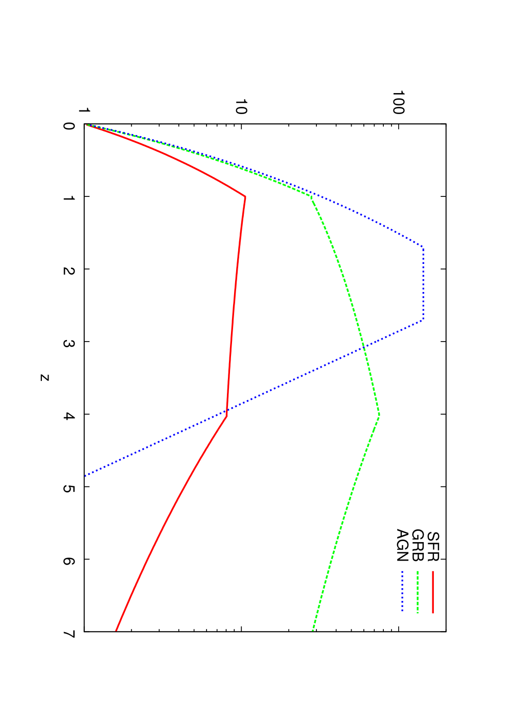
We also consider separately three particular source evolution models in which astrophysical sources of UHECR are assumed to have the evolution functions of either the star formation rate (SFR), or the gamma-ray burst (GRB) rate, or the active galactic nuclei (AGN) rate in the Universe. In this case,
| (3) |
As in Ref. [38] for SFR we take [39]
| (4) |
for GRB we take [40], thus
| (5) |
and for AGN we take the function [41, 42]
| (6) |
These evolution functions are shown in Fig. 1. The redshift-distance relation is computed with the usual values for the cosmological parameters: km s-1 Mpc-1 for the Hubble constant, for the dark energy density (in units of the critical density) and for the dark matter density.
As upper limit to the predicted VHE gamma-ray fluxes we use both the First-Year Fermi extragalactic diffuse background [26] and a calculation of the background in Ref. [27] which is lower than the first one in the 10-400 GeV energy range. Both fluxes are shown respectively in black and red in Figs. 2, 3 and 5. The analysis Ref. [27] using 2.5 years of the Fermi/LAT telescope, was done at high galactic latitudes using the same galactic model of the Fermi analysis. The estimation of the remaining diffuse cosmic ray flux was done with the prescription of the Fermi analysis, with the difference that the estimation of the suppression of the gamma-ray flux of the events classified as class 4 (those which are most confidently identified with -rays) was done independently of the analysis of the signal from known blazars. With this analysis the diffuse background at energies GeV has a different spectrum than that of the First-Year Fermi analysis [26]. The new spectral shape as function of energy closely follows the stacked spectrum of BL Lac objects, which dominate the point source contribution at largest energies. As we show below, the use of the VHE -ray flux in Ref. [27] instead of the original First-Year Fermi background makes a significant difference in terms of the largest cosmogenic neutrino fluxes allowed.
3 Comparison with Other Calculations
In Figs. 2 and 3 we compare the results of our program with those of other recent calculations of cosmogenic neutrino and VHE -ray fluxes.
In Ref. [29] the cascade evolution was computed both analytically and with a Monte Carlo simulation program [43], assuming a pure-proton composition model described by the parameters , , and defined as in Eqs. 1 and 2 above. In Fig. 2 we compare the photon and neutrino fluxes summed over flavors obtained with our code with those presented in the Figure 2 of Ref. [29]. We use the same parameters defining the emission model, namely , eV, and in Eq. 2 and the same EBL model [44] as in Ref. [29]. The discrete points taken from Ref. [29] and reproduced in Fig. 2 were obtained with the Monte Carlo method. With the chosen values of the parameters the resulting proton spectrum does not fit well the HiRes data, thus, we just normalized the proton flux to the HiRes spectrum above eV. Fig. 2 shows that the proton and neutrino fluxes are in moderate agreement but the VHE photon flux predictions in the energy range measured by Fermi/LAT differ roughly by factor of .


Ref. [30] also studied all-proton models of UHECR using an analytic model for the cascade evolution and fitted the resulting proton spectrum to the HiRes data. The injection spectrum Ref. [30] is again characterized by the parameters , , and , as in Eqs. 1 and 2 above. In Fig. 3 we compare the results of our photon flux and neutrino flux (summed over flavors) calculations with those presented in Figure B.7 of Ref. [30] with the same parameters, i.e. , eV, and . These are parameters that do not fit well the HiRes spectrum and are use just for the purpose of comparing results. We also use the same EBL model[33] as in [30]. Fig. 3 shows that our predictions for photon and neutrino fluxes are in very good agreement with those of Ref. [30].
4 Range of Cosmogenic Neutrino Fluxes in the Dip Model of UHECR
In this section we present the range of cosmogenic neutrino fluxes predicted by the dip model computed with a method similar to that described in Ref. [10], but with some differences. In particular we use two goodness of fit tests, one using Pearson’s chi-square and the other using the Poisson likelihood function.


Our procedure is the following. Among all models characterized by the emission spectrum parameters and source evolution models defined above we choose those which:
1)- produce proton fluxes which fit the HiRes spectrum [25, 11] at energies (for the dip model eV), taking into account the empty bins in the HiRes data above the highest energy UHECR events observed,
2)- produce proton fluxes not exceeding the HiRes spectrum at and
3)- produce VHE -ray fluxes not exceeding the measured background assumed,
at the 95% confidence level. We choose the value of the parameter in Eq. 1, i.e. the amplitude of the injected spectrum, by minimizing the combined . As just mentioned, the HiRes spectrum below and the measured extragalactic VHE gamma-ray fluxes are taken as upper limits to the predicted proton and gamma-ray fluxes respectively. Namely, if the predicted proton fluxes below and VHE gamma-ray fluxes exceed their respective measured values, they are included in the calculation of the . If not, they are not included (so the number of data points in the calculation changes in principle with each model). In this step we combine the high energy cosmic ray bins with number of event smaller than 5 into bins containing more than 5 events to ensure that Pearson’s statistics is valid. We keep only models with a -value . For these models, using the same fixed value of we calculate separately the goodness of fit for the bins with small number of events. Namely, we compute the Poisson likelihood function for the given value of . We then compute using a Monte Carlo technique the goodness of the fit or -value defined as the fraction of generated hypothetical experiments (observed spectra) with the same average number of evens (i.e. the predicted number) in each bin which results in a worse, namely a lower Poisson likelihood than the original one. This procedure for large number of events in each bin is equivalent to taking the distribution without free parameters. Only if the second value obtained in this way is also larger than 0.05 the model is accepted (notice that a higher value corresponds to a better fit, since more hypothetical experimental results would yield a worse fit than the one we obtained). In this way we eliminate those models which are inconsistent with the HiRes observed spectrum above and upper limits on the UHECR flux below this energy and the VHE -ray flux at the 95 % C.L.


As an example of our procedure in Fig. 4 we show the chi-square -value obtained in the first goodness of fit evaluation step described above of dip models with eV and varied from 2.00 to 2.70 in 0.05 steps for the injected spectrum and assuming the evolution function of Eq. 2 with varied from 0 to 5 in 0.5 steps. The -values are shown in a color coded logarithmic scale, from best () to worse ( close to zero). Only models with log() are accepted in the following. The only difference between the three panels in Fig. 4 is the upper bound on the predicted VHE -ray fluxes imposed: in 4.a-(upper panel) no upper limit is imposed, in 4.b-(middle panel) the First-Year Fermi spectrum is taken as upper limit and in 4.c-(lower panel) the spectrum of Ref. [27] is taken as upper limit. Note that models with allowed in 4.a are forbidden when the upper limit on the VHE photons fluxes is imposed in 4.b. The more stringent constraint on the diffuse -ray fluxes in 4.c is more restrictive than the First-Year Fermi spectrum for . Notice in particular that the best fit models of the middle panel, with and between 2.4 and 2.5 are rejected in the right panel. We can very easily see why this is so in Fig. 5, where we show the predicted cosmic ray, gamma ray and neutrino fluxes for the model with eV, and , which is the best (largest -value) model of Fig. 4.b and is rejected in Fig. 4.c. We see in Fig. 5 that the predicted -ray spectrum saturates the First-Year Fermi diffuse spectrum (shown in black) but exceeds the lower background estimate of Ref. [27]. The flux of photons produced only through the GZK process in this model is also shown in the figure (magenta dotted line). As in all models with , the dominant photon flux comes from pair production processes. Fig. 5 shows also the VHE -ray spectrum (magenta dot-dashed line) that the model would predict if the older evaluation of the EBL of Ref. [46] (still valid in the scenario of Ref. [47]) would be used. In this case the model would be somewhat less constrained by the upper bound on VHE photon fluxes. Besides, for maximal fluxes, the -rays above and below 10 GeV would require additional explanations.
In Figs. 6, 7 and 8 we show the range of cosmogenic neutrino fluxes averaged over flavors as function of the energy expected in the dip model of UHECR when fixing one of the parameters of the model. The fluxes shown with thick lines correspond to the VHE -ray background evaluation of Ref. [27] and they are lower than the fluxes shown with thin lines, which correspond to the First-Year Fermi VHE -ray spectrum. The results with the First-Year Fermi VHE -ray spectrum are compared with those of the new lower evaluation of Ref. [27] only in the left panels of Figs. 6, 7 and 8. Notice that in almost all cases only the maximum fluxes depend on the VHE -ray background assumed, because the lower neutrino fluxes are associated with VHE -ray fluxes much smaller that the upper bound. In this case there are only three lines for each model, two for maximum fluxes and one for the minimum fluxes. The range of fluxes is obtained by choosing among all the models with those with maximum and minimum neutrinos fluxes at each energy, thus the models which provide the fluxes shown may change at each energy value.
In the left panels of Figs. 6, 7 and 8, we take into account possible systematic errors in the HiRes energy scale, by shifting the energy scale by a factor in the range to 1.30 (and the results of both VHE -ray backgrounds are shown). In the right panels of Figs. 6, 7 and 8 the ranges of neutrino fluxes with and without shifting the HiRes energy scale are compared for the particular case yielding the largest fluxes with the new VHE -ray spectrum of Ref. [27]. The neutrino flux ranges obtained varying the energy are larger than with the energy fixed, but not by much. This is so because the HiRes spectrum without any energy shift is very well fitted by the dip-model, so large changes in the HiRes spectrum do not provide a good fit.
In Fig. 6.a (left panel) is either fixed to eV or varied within its assumed range, from eV up to eV, and as well as in the evolution function in Eq. 2 are varied as explained above (and the HiRes energy is varied too). Notice that for each energy there are only three lines, the highest corresponding to the maximum fluxes allowed by the First-Year Fermi -ray background. The maximum neutrino fluxes with the new -ray background evaluation of Ref. [27] are about a factor of 2 smaller. In Fig. 6.b (right panel) we compare the neutrino flux range obtained by shifting the HiRes energy scale as presented in the left panel (larger range) with the range obtained without any energy shift, for all up to eV and the VHE -ray spectrum of Ref. [27]. As Fig. 6.b shows,the difference in the ranges derived by allowing a variation of the HiRes energy scale and by kipping it fix is very small. Notice that the models with eV in the left panel, are not allowed when the HiRes energy scale is not shifted, as shown in the right panel.
In Fig. 7 the source evolution parameter in Eq. 2 is fixed and all other parameters varied. Models with or 1 are disfavored (see e.g. Fig 4), and those with forbidden by the new -ray upper limits, thus neutrino flux ranges are presented in Fig. 7.a (left panel) for and (and the HiRes energy varied as explained above). In 7.b (right panel) we compare the range obtained by shifting the HiRes energy as in the left panel (larger range) with the range obtained without any energy shift for and the VHE -ray spectrum of Ref. [27] only. For , the case with larger fluxes in the left panel, no allowed range remains without an energy shift. Thus we present in 7.b the case with the largest neutrino fluxes for which both ranges (i.e. with and without energy shift) exist, which is the case of .
In Fig. 8 one of the specific source evolution functions in Eqs. 4, 5 and 6 is chosen for each range and and are varied as explained before. Notice that these evolution functions were not included in the previous two figures. Fig. 8.a (left panel) shows that dip models with the AGN evolution function of Eq. 6 are rejected by both VHE -ray background evaluations we take as upper bounds to the gamma-ray fluxes produced and dip models with the GRB evolution in Eq. 5 are not allowed by the lower VHE -ray spectrum of Ref. [27]. Thus, Fig. 8.a shows the range of neutrino fluxes for the SFR evolution function in Eq. 4 for both VHE -ray spectra. Only the maximum fluxes change with the VHE -ray spectrum. The minimum fluxes are independent of the upper limit provided by VHE -rays. The range, which is higher, corresponding to the GRB evolution is presented only for the First-Year Fermi VHE -ray spectrum because no range remains.
As in the left panels of the previous two figures, Fig. 8.a shows the maximum and minimum cosmogenic neutrino fluxes obtained by also varying the HiRes energy scale. In 8.b (right panel) we compare the range obtained by shifting the energy scale of the HiRes spectrum as in the left panel (larger range) with the range obtained without any energy shift only for the SFR evolution of Eq. 4, the only one of the three considered allowed by the VHE -ray spectrum of Ref. [27] which is assumed in this panel.


Figs. 6, 7 and 8 also show the atmospheric neutrino flux measured by IceCube [48], existing experimental upper limits from Auger [49], ANITA II [50] and IceCube-40 and expected sensitivity regions for IceCube in 3 years [51], JEM-EUSO [52] and ARA [53]. The JEM-EUSO bound corresponds to 1 event per energy decade per year. All the others are 90% CL bounds according to the respective references. The differential flux bound corresponding to 3 years of observation of IceCube was not provided by the IceCube collaboration. It was obtained by scaling down the IceCube-40 differential flux bound by the ratio of the integrated limits (which assume an neutrino spectrum) shown in Fig. 3 of Ref. [51]. This procedure does not take into account the presence of the atmospheric neutrino background and thus it is not correct at low energies, but it should be fine in the energy region where the cosmogenic neutrino fluxes are maximal. Notice that of all the expected sensitivities shown only that corresponding to 3 years of observation with ARA enter into the cosmogenic neutrino ranges shown. The maximum cosmogenic neutrino fluxes are a factor of 2 or 3 below the sensitivity of IceCube in 3 years. Thus at least about 10 years of observation with IceCube or a similar KM3NeT detector would be needed for detection.
5 Range of Cosmogenic Neutrino Fluxes in the Ankle Model of UHECR
Because we are interested in producing upper bounds to the cosmogenic neutrinos fluxes, we also consider what in Ref. [29] is called the “ankle model”, in which we fit with protons the HiRes spectrum only above eV. This is not a self consistent model, since it does not explain the UHECR data below this energy. An additional component of UHECR needs to be introduced. The nature of this extra component will dictate if there is an additional contribution to the -ray flux. If it is dominated by extragalactic protons, we will have a more complicated version of a “dip”-like model, in which there would be a large contribution to the -ray background and, as a result, lower allowed maximum neutrino fluxes. Galactic protons would contradict the isotropy of the observed UHECR flux. The only other possibility are heavier nuclei, either galactic or extragalactic. But this would contradict the composition measurements of both HiRes and Auger [7, 2].
We assume in this model that the cutoff energy in the emission spectrum (see Eq.1) is eV. The neutrino flux ranges are then obtained as explained in the previous section. The ankle model was also studied in Refs. [29] and [30] and found to produce larger neutrino fluxes.
The range of fluxes are shown in Fig. 9. The three panels of Fig. 9 are similar to Figs. 6.a, 7.a and 8.a except for the higher values of and . In Fig. 9.a (upper panel) is fixed and as well as in the evolution function in Eq. 2 are varied as explained above. In Fig. 9.b (middle panel) the source evolution parameter in Eq. 2 is fixed and all other parameters varied. In Fig. 9.c (lower panel) one of the specific source evolution functions in Eqs. 4, 5 and 6 is chosen for each range and and are varied as explained before. In all three panels the HiRes energy has been varied as explained above.
Fig. 9.c shows that in the ankle model, both the GRB and AGN source evolution functions are allowed, even with the lower -ray background we used. For the AGN evolution, only a very small range of parameters are allowed, so that the maximum and minimum neutrino fluxes (shown in thick magenta dot-dashed lines) practically coincide.
The maximum neutrino fluxes are here a factor of 2 to 3 larger than in the dip model, which puts them within the reach of IceCube in three years of observation.
6 Conclusions
Cosmogenic neutrinos constitute one of the main high energy signals expected in neutrino telescopes, such as IceCube [19], ANITA [20], the future KM3NeT [21] and ARA [22] or space based observatories such as JEM-EUSO [23]. They could also be observed by Pierre Auger Observatory [1] and the Telescope Array [24]. Here we present the largest neutrino fluxes compatible with cosmic rays and gamma-rays observations.
Proton primaries produce larger maximum cosmogenic neutrino fluxes than heavier nuclei. Thus we consider the dip model, which assumes that all UHECR primaries above 1018 eV are protons and is consistent with both the spectrum and composition data of HiRes. As it has been already pointed out [29, 30] fitting the UHECR spectrum with protons only above higher energies, such as 1019 eV, leads to higher neutrino fluxes. This, however, is an incomplete model of UHECR unless a consistent explanation of the dominant component below this energy is presented. With this caveat, we also consider this model, which following Ref. [29] we call the ankle model, to obtain the highest allowed cosmogenic neutrino fluxes.
We use a program which allows for fast analytic calculations of the secondary proton, photon and neutrino spectrum to find at each energy the expected range of cosmogenic neutrino fluxes. We require the produced UHECR spectrum to fit the HiRes spectrum at energies above a certain energy , which is 1018 eV in the dip model and 1019 eV in the ankle model. Below this energy, the HiRes spectrum is taken as an upper bound. We also impose as an upper bound to the predicted gamma-ray fluxes the new evaluation of the diffuse extragalactic VHE -ray background of Ref. [27] and compare the results with those derived assuming instead the First-Year Fermi [11] background, which is higher than the former by about a factor of 2 at energies above 10 GeV.
The resulting neutrino flux ranges are presented in Figs. 6 to 9 together with experimental bounds of IceCube-40, Auger and ANITA and sensitivity regions of IceCube in 3 years, ARA in 3 years and JEM-EUSO.
In the left panels of Figs. 6, 7 and 8 we show the range of cosmogenic neutrino fluxes as function of the energy expected in the dip-model of UHECR allowing for a shift of the HiRes energy scale by a factor between and 1.30, to take into account possible systematic errors. Also in these panels the results obtained by taking as upper bounds both VHE -ray backgrounds are compared. The comparison of the ranges of neutrino fluxes obtained in the dip model with and without shifting the nominal HiRes energy are presented in the right panels of Figs. 6, 7 and 8 for the particular case yielding the largest fluxes with the new VHE -ray spectrum of Ref. [27] in the corresponding left panel of the same figure. The ranges obtained varying the energy are larger than with the energy fixed, but not by much, because the HiRes spectrum without any energy shift is very well fitted by the dip model, so large changes in the HiRes spectrum do not provide good fits.
In Figs. 6 and 7, the evolution model in Eq. 2 is used. In these figures, the highest cosmogenic neutrino fluxes allowed by the lower estimate of the VHE -ray background [27] are about a factor of 2 lower that those obtained by imposing the First-Year Fermi background.
Figs. 6, 7 and 8 show that detecting the highest cosmogenic neutrino fluxes predicted by the dip model would require about 10 years of observation with IceCube (or a similar KM3NeT) or the construction of the new ARA detector.
The upper and middle panels of Fig. 9 are similar to the left panels of Figs. 6 and 7 but apply to the ankle model. Here the maximum cosmogenic neutrino fluxes are a factor of 2 to 3 higher than in the dip model, what brings them into the range of detectability of IceCube in 3 years. Our conclusions are consistent with those of Ref. [30] in that the ankle model produces maximal neutrino fluxes which could be detected with a few years of observation of IceCube, and are not consistent with those of Ref. [29] in this regard.
Refs. [29] and [30] use the evolution model in Eq. 2. We also consider here the special evolution functions in Eqs. 4, 5 and 6, in which the UHECR sources are assumed to have the same evolution of either the star formation rate (SFR), or the gamma-ray burst (GRB) rate, or the active galactic nuclei (AGN) rate in the Universe. To our knowledge the limits imposed by the diffuse extragalactic VHE -ray background extracted from Fermi-LAT data on these evolution functions had not been studied before.
Fig. 8 shows that the new VHE -ray background [27] rejects the dip models assumed to have the GRB source evolution function in Eq. 5. The dip models with the AGN source evolution function in Eq. 6 are rejected by any of the two VHE -ray backgrounds, so models with this evolution do not appear in the figure. Only dip models with the SFR evolutions function in Eq. 4 is allowed by both observed VHE -ray backgrounds assumed, and both ranges (only the maximum fluxes change) are very similar. The lower panel of Fig. 9 shows that in the ankle model, both the GRB and AGN source evolution functions are allowed, even with the lower -ray background we used (in the case of the AGN evolution barely so).
Acknowledgments The numerical calculations in this work were performed with the Computational Cluster of the Theoretical Division of INR RAS. G.G was supported in part by the US DOE grant DE-FG03-91ER40662 Task C. O.K. was supported in part by the RFBR grant 10-02-01406-a. G.G. wants to thank the APC, Paris, for its hospitality during part of the period in which this paper was written.
References
- [1] The Pierre Auger Observatory, http://www. auger.org.
- [2] J. Abraham et al. [Pierre Auger Collaboration], Phys. Rev. Lett. 104, 091101 (2010); [arXiv:1002.0699 [astro-ph.HE]].
- [3] J. Abraham et al. [Pierre Auger Collaboration], Science 318, 938 (2007) [arXiv:0711.2256 [astro-ph]]; J. Abraham et al. [Pierre Auger Collaboration], Astropart. Phys. 29, 188 (2008) [Erratum-ibid. 30, 45 (2008)] [arXiv:0712.2843 [astro-ph]]; P. Abreu et al. [Pierre Auger Observatory Collaboration], Astropart. Phys. 34, 314 (2010) [arXiv:1009.1855 [Unknown]].
- [4] G. Giacinti, M. Kachelriess, D. V. Semikoz and G. Sigl, JCAP 1008, 036 (2010) [arXiv:1006.5416 [astro-ph.HE]]; D. V. Semikoz, arXiv:1009.3879 [astro-ph.HE]; G. Giacinti and D. V. Semikoz, Phys. Rev. D 83, 083002 (2011) [arXiv:1011.6333 [astro-ph.HE]].
- [5] The High Resolution Fly’s Eye Collaboration (HiRes), http://hires.physics.utah.edu/
- [6] J. Belz [HiRes Collaboration], Nucl. Phys. Proc. Suppl. 190 (2009) 5. R. U. Abbasi et al. [HiRes Collaboration], Phys. Rev. Lett. 104, 161101 (2010) [arXiv:0910.4184 [astro-ph.HE]].
- [7] R. U. Abbasi et al. [The High Resolution Fly’s Eye Collaboration], Astrophys. J. 622, 910 (2005) [arXiv:astro-ph/0407622]; D. R. Bergman et al., “UHECR composition measurements using the HiRes-II detector,” Proc. 29th ICRC (Pune), 2005 [astro-ph/0507483].
- [8] R. U. Abbasi et al., Astropart. Phys. 30, 175 (2008) [arXiv:0804.0382 [astro-ph]] and arXiv:1002.1444 [astro-ph.HE].
- [9] C. T. Hill and D. N. Schramm, Phys. Rev. D 31, 564 (1985); V. S. Berezinsky and S. I. Grigorieva, Astron. Astrophys. 199 (1988) 1; V. Berezinsky, A. Z. Gazizov and S. I. Grigorieva, Phys. Rev. D 74, 043005 (2006) [arXiv:hep-ph/0204357]; astro-ph/0210095; Nucl. Phys. Proc. Suppl. 136, 147 (2004) [astro-ph/0410650]; Phys. Lett. B 612 (2005) 147 [astro-ph/0502550].
- [10] G. Gelmini, O. Kalashev and D. V. Semikoz, Astropart. Phys. 28, 390 (2007) [arXiv:astro-ph/0702464] and arXiv:0706.3847 [astro-ph].
- [11] R. U. Abbasi et al. [HiRes Collaboration], Phys. Rev. Lett. 100, 101101 (2008) [arXiv:astro-ph/0703099].
- [12] J. Abraham et al. [Pierre Auger Collaboration], Phys. Rev. Lett. 101, 061101 (2008) [arXiv:0806.4302 [astro-ph]]. J. Abraham et al. [The Pierre Auger Collaboration], Phys. Lett. B 685, 239 (2010) [arXiv:1002.1975 [astro-ph.HE]].
- [13] K. Greisen, Phys. Rev. Lett. 16, 748 (1966). G. T. Zatsepin and V. A. Kuzmin, JETP Lett. 4, 78 (1966) [Pisma Zh. Eksp. Teor. Fiz. 4, 114 (1966)].
- [14] V. S. Berezinsky and G. T. Zatsepin, Phys. Lett 28B, 423 (1969).
- [15] G. Gelmini, O. E. Kalashev and D. V. Semikoz, J. Exp. Theor. Phys. 106, 1061 (2008) [arXiv:astro-ph/0506128]; G. B. Gelmini, O. E. Kalashev and D. V. Semikoz, JCAP 0711, 002 (2007) [arXiv:0706.2181 [astro-ph]].
- [16] J. Abraham et al. [Pierre Auger Collaboration], Astropart. Phys. 29, 243 (2008). [arXiv:0712.1147 [astro-ph]]. J. Abraham et al. [The Pierre Auger Collaboration], Astropart. Phys. 31, 399 (2009); [arXiv:0903.1127 [astro-ph.HE]].
- [17] O. E. Kalashev, V. A. Kuzmin, D. V. Semikoz and G. Sigl, Phys. Rev. D 66, 063004 (2002) [arXiv:hep-ph/0205050].
- [18] D. V. Semikoz and G. Sigl, JCAP 0404, 003 (2004) [arXiv:hep-ph/0309328].
- [19] IceCube, http://icecube.wis.edu/.
- [20] Antarctic Impulse Transient Array (ANITA), http:// www.ps.uci.edu/anita/.
- [21] Cubic Kilometre Neutrino Telescope (KM3NeT), http:// www.km3net.org/home.php
- [22] Askaryan Radio Array (ARA), http://ara.physics.wisc. edu/
- [23] Extreme Universe Space Observatory onboard the Japa nese Experiment Module (JEM-EUSO), http://jemeuso. riken.jp/en/index.html
- [24] Telescope Array (TA), http://www.telescopearray.org/
- [25] http://www.physics.rutgers.edu/%7Edbergman/HiRes-Monocular-Spectra-200702.html
- [26] A. A. Abdo et al. [The Fermi-LAT collaboration], Phys. Rev. Lett. 104, 101101 (2010) [arXiv:1002.3603 [astro-ph.HE]].
- [27] A. Neronov and D. V. Semikoz, arXiv:1103.3484 [astro-ph.CO].
- [28] J. Wdowczyk , W. Tkaczyk, C. Adcock and A. W. Wolfendale, J. Phys. A: Gen. Phys 4 L37-9 (1971); J. Wdowczyk , W. Tkaczyk and A. W. Wolfendale, J. Phys. A: Gen. Phys 5 1419 (1972); V. Berezinsky and A. Yu. Smirnov, Astrophys. Sp. Sci. 32, 461 (1975); J. Wdowczyk and A. W. Wolfendale, Astrophys. Jour. 349, 35 (1990);
- [29] V. Berezinsky, A. Gazizov, M. Kachelriess and S. Ostapchenko, Phys. Lett. B 695, 13 (2011) [arXiv:1003.1496 [astro-ph.HE]].
- [30] M. Ahlers, L. A. Anchordoqui, M. C. Gonzalez-Garcia, F. Halzen and S. Sarkar, Astropart. Phys. 34, 106 (2010) [arXiv:1005.2620 [astro-ph.HE]].
- [31] O.E. Kalashev, V.A. Kuzmin and D.V. Semikoz, astro-ph/9911035; Mod. Phys. Lett. A 16, 2505 (2001) [astro-ph/0006349]. O.E. Kalashev Ph.D. Thesis, INR RAS, 2003.
- [32] P. Bhattacharjee, G. Sigl, Phys. Rept. 327, 109 (2000).
- [33] A. Franceschini, G. Rodighiero and M. Vaccari, Astron. & Astrophys. 487 837 (2008) [arXiv:0805.1841].
- [34] T. M. Kneiske and H. Dole, Astron. & Astrophys. 515 A19 (2010) [arXiv:1001.2132].
- [35] A. Dominguez et al., MNRAS 410 2556 (2010) [arXiv:1007.1459].
- [36] K. Dolag, D. Grasso, V. Springel and I. Tkachev, JCAP 0501, 009 (2005). [astro-ph/0410419].
- [37] A. Neronov and D. V. Semikoz, Phys. Rev. D 80, 123012 (2009) [arXiv:0910.1920 [astro-ph.CO]].
- [38] X. Wang, R. Liu, F. Aharonian, arXiv:1103.3574 [astro-ph.HE]
- [39] H. Yüksel, M. D. Kistler, J. F. Beacom and A. M. Hopkins, Ap. J. 638 L5 (2008).
- [40] H. Yüksel and M.D. Kistler Phys. Rev. D 75, 083004 (2007).
- [41] G. Hasinger, T. Miyaji, M. Schmidt, Astron. and Astroph. 441 417 (2005)
- [42] M. Ahlers, L. A. Anchordoqui and S. Sarkar, Phys. Rev. D 79, 083009 (2009) [arXiv:0902.3993 [astro-ph.HE]].
- [43] M. Kachelriess and D. Semikoz, Astropart. Phys. 23, 486 (2005) [arXiv:astro-ph/0405258]; M. Kachelriess, S. Ostapchenko and R. Tomas, New J. Phys. 11, 065017 (2009) [arXiv:0805.2608 [astro-ph]].
- [44] T. M. Kneiske, T. Bretz, K. Mannheim and D. H. Hartmann, Astron. Astrophys. 413, 807 (2004) [arXiv:astro-ph/0309141].
- [45] S. Baker and R.D. Cousins, Nucl. Instrum. Methods 221, 437 (1984); Particle Data Group’s Statistics Review (2004).
- [46] F. W. Stecker, M. A. Malkan and S. T. Scully, Astrophys. J. 648, 774 (2006) [arXiv:astro-ph/0510449].
- [47] W. Essey and A. Kusenko, Astropart. Phys. 33, 81 (2010) [arXiv:0905.1162 [astro-ph.HE]]; W. Essey, O. E. Kalashev, A. Kusenko and J. F. Beacom, Phys. Rev. Lett. 104, 141102 (2010) [arXiv:0912.3976 [astro-ph.HE]].
- [48] R. Abbasi et al. [IceCube Collaboration], arXiv:1104.5187 [astro-ph.HE].
- [49] J. Abraham et al. [Pierre Auger Collaboration], Phys. Rev. D 79, 102001 (2009) [arXiv:0903.3385 [astro-ph.HE]].
- [50] P. W. Gorham et al. [The ANITA Collaboration], Phys. Rev. D 82, 022004 (2010) [arXiv:1003.2961 [astro-ph.HE]]; Erratum: arXiv:1011.5004 [astro-ph.HE].
- [51] R. Abbasi et al. [IceCube Collaboration], Phys. Rev. D 83, 092003 (2011) [arXiv:1103.4250 [astro-ph.CO]].
- [52] N. Inoue, K. Miyazawa and Y. Kawasaki [JEM-EUSO Collaboration], Nucl. Phys. B (Proc. Suppl.) 196 135 (2009).
- [53] P. Allison et al., arXiv:1105.2854 [astro-ph.IM].