跳到论文正文
W Papers独立论文阅读器 arXiv:1107.1584 论文正文 计算阅读时间 · 0%
引用这篇论文根据当前论文元数据生成,正式投稿前建议核对。


License: arXiv.org perpetual non-exclusive license
arXiv:1107.1584v3 [math.AG] 24 Sep 2012

Approximate Parametrization of Space Algebraic CurvesThanks:  This work has been developed, and partially supported, by the Spanish ”Ministerio de Ciencia e Innovación” under the Project MTM2008-04699-C03-01, and by the ”Ministerio de Economía y Competitividad” under the project MTM2011-25816-C02-01. All authors belong to the Research Group ASYNACS (Ref. CCEE2011/R34).

Sonia L. Rueda Affiliation: Dpto. de Matemática Aplicada Affiliation: E.T.S. Arquitectura, Universidad Politécnica de Madrid Affiliation: E-28040 Madrid, Spain Email: sonialuisa.rueda@upm.es    Juana Sendra Affiliation: Dpto. de Matemática Aplicada a la I.T. de Telecomunicación Affiliation: E.U.I.T.Telecomunicación, Universidad Politécnica de Madrid Affiliation: E-28031 Madrid, Spain Email: jsendra@euitt.upm.es    J. Rafael Sendra Affiliation: Dpto. de Matemáticas Affiliation: Universidad de Alcalá Affiliation: E-28871 Madrid, Spain Email: rafael.sendra@uah.es
Abstract

Given a non-rational real space curve and a tolerance ϵ>0\epsilon>0, we present an algorithm to approximately parametrize the curve. The algorithm checks whether a planar projection of the space curve is ϵ\epsilon-rational and, in the affirmative case, generates a planar parametrization that is lifted to an space parametrization. This output rational space curve is of the same degree as the input curve, both have the same structure at infinity, and the Hausdorff distance between them is always finite.

Introduction

The development of approximate algorithms for algebraic and geometric problems is an active research area (see e.g. [21] and [23]) that focuses on different problems as, for instance, the computation of gcds (see [4], [10], [16]), the factorization of polynomials ([6], [12], [15]), the implicicitization of surfaces ([7], [9]), the parametrization of curves and surfaces ([2], [11], [14], [17], [18], [20]), etc. These approximate algorithms are applicable by themselves since they face symbolic computation to real world problems. Moreover, those of geometric nature are of special interest in the field of CAGD. For instance, providing parametric representations of algebraic geometric objects helps in some CAGD constructions as surface–-surface intersection or computation of planar sections (see e.g. Example 5.3. in [20]).

In this context, when using the term ”approximate”, there is certain risk of ambiguity since it can have a double meaning (see e.g. [24]). Let us clarify what we mean in our case. Here, as in our previous papers [17], [18], [20], with the term ”approximate” we do not mean ”numerical” but something different (see introduction to [20] for further details): our input is the perturbation of an unknown input; once the perturbation is received we treat it exactly to provide an output that is close (in this sense it is ”approximate”), under certain distance, to the theoretical output of the unperturbed unknown input.

More precisely, the problem in this paper is as follows. Let 𝒞∗{\mathcal{C}}^{*} be a rational real space curve defined as the complex-zero set of a finite set ℳ⊂ℝ⁡[x,y,z]{\cal M}\subset{\mathbb{R}}[x,y,z] of real polynomials; in practice card⁡(ℳ)=2{\rm card}({\cal M})=2. Nevertheless, instead of getting ℳ{\cal M} as input of our problem, we get a new finite subset ℱ⊂ℝ⁡[x,y,z]{\cal F}\subset{\mathbb{R}}[x,y,z] (which is a perturbation of ℳ\cal M) of real polynomials that defines a new curve 𝒞{\mathcal{C}}, obviously different to 𝒞∗{\mathcal{C}}^{*}. Since the genus of a curve is unstable under perturbations, the input curve 𝒞{\mathcal{C}} will have positive genus and hence it will not be parametrizable by rational functions. Ideally, the problem would consists in finding the initial curve 𝒞∗{\mathcal{C}}^{*} or, even better, a rational parametrization of it. However, this goal is unrealistic. Instead, one might require to find a rational parametrization of the closest rational curve to 𝒞{\mathcal{C}} under certain distance; say, under the Hausdorff distance. Nevertheless, in this paper we deal with a weaker statement of the problem. Namely, finding a rational parametrization of one rational space curve being close (in comparison to a given tolerance ϵ>0\epsilon>0) to 𝒞{\mathcal{C}} under the Hausdorff distance. Our statement, although may not yield to the best output rational curve, generates one good answer. This can be seen as a first step for the harder, more general, and theoretical problem of finding the best (in the sense of closest) rational curve being, our solution, meanwhile ready to be used in applications.

In [17], the authors show how to solve the problem for the particular case of ϵ\epsilon-monomial plane curves (i.e. plane curves having an ϵ\epsilon-singularity of maximum ϵ\epsilon-multiplicity); see also [18] for the case of surfaces. Later, in [20], the problem was solved for the more general case of ϵ\epsilon-rational plane curves. The current paper is, therefore, the natural continuation of this research since it deals with the next step, namely the case of space curves.

In the unperturbed case, the problem can be solved by birationally projecting the space curve on a plane, checking the genus of the projected curve and, in case of genus zero, parametrizing the plane curve to afterwards inverting the parametrization to a rational parametrization of the input curve (see e.g. [22] for further details). Now, the situation is more complicated. More precisely the strategy (see box below) is as follows.

  Let 𝒞⊂ℝ3      We get 𝒞¯, parametrized by 𝒫⁡(t)=(p1​(t)q⁡(t),p2​(t)q⁡(t),p3​(t)q⁡(t)), and close to 𝒞.        General Strategy        under a suitable projection (say πz onto the plane z=0) we project 𝒞.   ↺   Applying Chinese Remainder techniques, we lift 𝒟.          We get a plane curve πz​(𝒞) satisfying the hypotheses in [20].        We compute the ϵ-genus of πz​(𝒞); say it is zero.        Algorithm in [20] outputs a rational curve 𝒟, parametrized as 𝒬⁡(t)=(p1​(t)q⁡(t),p2​(t)q⁡(t)), and close to πz​(𝒞).   {\small{\framebox{$\begin{array}[]{ccccc}{\framebox{\parbox{56.9055pt}{Let ${\mathcal{C}}\subset{\mathbb{R}}^{3}$ } }}&&&&{\framebox{\parbox{128.0374pt}{We get $\overline{{\mathcal{C}}}$, parametrized by ${\mathcal{P}}(t)=(\frac{p_{1}(t)}{q(t)},\frac{p_{2}(t)}{q(t)},\frac{p_{3}(t)}{q(t)})$, and close to ${\mathcal{C}}$. } }}\\ $\vector{0}{-1}{20.0}$&&{\framebox{\parbox{79.6678pt}{{\sf General Strategy}} }}&&\begin{array}[]{c}\\ \vector{0}{1}{20.0}\end{array}\\ {\framebox{\parbox{99.58464pt}{under a suitable projection (say $\pi_{z}$ onto the plane $z=0$) we project ${\mathcal{C}}$.} }}&&\mathbf{\circlearrowleft}&&{\framebox{\parbox{113.81102pt}{Applying Chinese Remainder techniques, we lift $\cal D$.} }}\\ $\vector{0}{-1}{20.0}$&&&&$\vector{0}{1}{20.0}$\\ {\framebox{\parbox{99.58464pt}{We get a plane curve $\pi_{z}({\mathcal{C}})$ satisfying the hypotheses in \cite[cite]{[\@@bibref{}{PRSS}{}{}]}.} }}&$\vector{1}{0}{12.0}$&{\framebox{\parbox{85.35826pt}{We compute the $\epsilon$-genus of $\pi_{z}({\mathcal{C}})$; say it is zero. } }}&$\vector{1}{0}{12.0}$&{\framebox{\parbox{128.0374pt}{Algorithm in \cite[cite]{[\@@bibref{}{PRSS}{}{}]} outputs a rational curve $\cal D$, parametrized as ${\mathcal{Q}}(t)=(\frac{p_{1}(t)}{q(t)},\frac{p_{2}(t)}{q(t)})$, and close to $\pi_{z}({\mathcal{C}})$.} }}\end{array}$}}}

We assume some conditions on the original space curve 𝒞{\mathcal{C}} (see Section 1) such that when it is projected onto a plane we get a curve satisfying the hypotheses required by the algorithm in [20]; let us denote by πz​(𝒞)\pi_{z}({\mathcal{C}}) the projected curve, so we are assuming w.l.o.g. in this explanation that projection has been performed on the plane z=0z=0. Then, the algorithm in [20] determines whether πz​(𝒞)\pi_{z}({\mathcal{C}}) is ϵ\epsilon-rational, where ϵ\epsilon is a fixed given tolerance. If πz​(𝒞)\pi_{z}({\mathcal{C}}) is not ϵ\epsilon-rational one may try a different projection, but here we simply ask the algorithm to terminate since, although in some examples this seems to work, we do not have any theoretical argumentation to ensure when that projection exists. Otherwise, the algorithm in [20] goes ahead and computes a rational parametrization 𝒬⁡(t){\mathcal{Q}}(t) of a plane rational curve 𝒟\cal D. The last step consists in lifting 𝒟\cal D to a rational space curve 𝒞¯\overline{{\mathcal{C}}} being close to 𝒞{\mathcal{C}}. For this purpose, we first realize that a sufficient condition for the finite Hausdorff distance requirement, between both curves, is given by the structure at infinity of the input curve 𝒞{\mathcal{C}}. Taking into account this fact, and using a Chinese-remainder type interpolation, we get a rational parametrization of 𝒞¯\overline{{\mathcal{C}}}. As a consequence of this process, we get a rational space curve 𝒞¯\overline{{\mathcal{C}}} of the same degree as 𝒞{\mathcal{C}}, having the same structure at infinity as 𝒞{\mathcal{C}}, and such that the Hausdorff distance between 𝒞¯\overline{{\mathcal{C}}} and 𝒞{\mathcal{C}} is finite.

The structure of the paper is as follows. In Section 1, we introduce the notation that will be used throughout the paper as well as the general assumptions. Moreover, we comment on the reasons for the inclusion of these assumptions, we discuss how to check them algorithmically, and we show that they (the assumptions) are general enough. Section 2 is devoted to the projected curve πz​(𝒞)\pi_{z}({\mathcal{C}}) and, more precisely, to prove that under the general assumptions imposed in 1 πz​(𝒞)\pi_{z}({\mathcal{C}}) satisfies all requirements in the algorithm in [20]. Section 3 focuses on how to lift the rational plane curve 𝒟\cal D (generated by applying the algorithm in [20] to πz​(𝒞)\pi_{z}({\mathcal{C}})) to the curve 𝒞¯\overline{{\mathcal{C}}} such that both curves, 𝒞{\mathcal{C}} and 𝒞¯\overline{{\mathcal{C}}}, have the same structure at infinity; note that πz\pi_{z} is a birational map between 𝒞{\mathcal{C}} and πz​(𝒞)\pi_{z}({\mathcal{C}}), but we are lifting 𝒟≠πz​(𝒞){\cal D}\neq\pi_{z}({\mathcal{C}}). In Section 4 we summarize these ideas to derive an algorithm that is illustrated by two examples. In Section 5, we prove that the Hausdorff distance between the input and output curves, of our algorithm, is always finite. For this purpose, we briefly study the asymptotes of space curves.

1 General Assumptions and Notation

We consider a computable subfield 𝕂{\mathbb{K}} of ℝ{\mathbb{R}}, as well as its algebraic closure 𝔽{\mathbb{F}}; in practice, we may think that 𝕂=ℚ{\mathbb{K}}={\mathbb{Q}}. We denote by 𝔽2{\mathbb{F}}^{2} and 𝔽3{\mathbb{F}}^{3} the affine plane an affine space over 𝔽{\mathbb{F}}, respectively. Similarly, we denote by ℙ2​(𝔽){\mathbb{P}}^{2}({\mathbb{F}}) and ℙ3​(𝔽){\mathbb{P}}^{3}({\mathbb{F}}) the projective plane and projective space over 𝔽{\mathbb{F}}, respectively. Furthermore, if 𝒜⊂𝔽3{\cal A}\subset{\mathbb{F}}^{3} (similarly if 𝒜⊂𝔽2{\cal A}\subset{\mathbb{F}}^{2}) we denote by 𝒜∗⊂𝔽3{\cal A}^{*}\subset{\mathbb{F}}^{3} its Zariski closure, and by 𝒜h⊂ℙ3​(𝔽){\cal A}^{h}\subset{\mathbb{P}}^{3}({\mathbb{F}}) the projective closure of 𝒜∗{\cal A}^{*}. We will consider (x,y,z)(x,y,z) as affine coordinates and (x:y:z:w)(x:y:z:w) as projective coordinates. Also, for 𝒜{\cal A} as above, we denote by 𝒜∞{\cal A}^{\infty} the intersection of 𝒜h{\cal A}^{h} with the projective plane of equation w=0w=0. In addition, for every polynomial H∈𝕂⁡[x,y,z]H\in{\mathbb{K}}[x,y,z] we denote by Hh​(x,y,z,w)H^{h}(x,y,z,w) the homogenization of HH.

Our method will be based on the projection of the space curve on a plane. Without loss of generality (see below) we will consider that z=0z=0 is the projection plane. So we introduce the map

πz:𝔽3→𝔽2,(x,y,z)↦(x,y),\pi_{z}:{\mathbb{F}}^{3}\rightarrow{\mathbb{F}}^{2},(x,y,z)\mapsto(x,y),

as well as

πzh:ℙ3(𝔽)∖{(0:0:1:0)}→ℙ2(𝔽),(x:y:z:w)↦(x:y:w).\pi_{z}^{h}:{\mathbb{P}}^{3}({\mathbb{F}})\setminus\{(0:0:1:0)\}\rightarrow{\mathbb{P}}^{2}({\mathbb{F}}),(x:y:z:w)\mapsto(x:y:w).

Our main object of study will be an irreducible (over 𝔽{\mathbb{F}}) affine real (non-planar) space curve 𝒞⊂𝔽3{\mathcal{C}}\subset{\mathbb{F}}^{3}. Although, in practice, in most cases, 𝒞{\mathcal{C}} will be given by two generators, we present the results for the general case where a finite set of generators is provided. Therefore, we assume that 𝒞{\mathcal{C}} is given as the zero-set (over 𝔽{\mathbb{F}}) of a finite set of real polynomials ℱ={F1,…,Fs}⊂𝕂⁡[x,y,z]{\cal F}=\{F_{1},\ldots,F_{s}\}\subset{\mathbb{K}}[x,y,z], s≥2s\geq 2. ϵ\epsilon will be the tolerance and we assume that 0<ϵ<10<\epsilon<1. In addition, we assume the following:

General Assumptions

  1. 1.

    The cardinality of 𝒞∞{\mathcal{C}}^{\infty} is deg⁡(𝒞){\rm deg}({\mathcal{C}}).

  2. 2.

    πz:𝒞→πz​(𝒞)∗\pi_{z}:{\mathcal{C}}\rightarrow\pi_{z}({\mathcal{C}})^{*} is birational and deg⁡(𝒞)=deg⁡(πz​(𝒞)∗){\rm deg}({\mathcal{C}})={\rm deg}(\pi_{z}({\mathcal{C}})^{*}).

  3. 3.

    (1:0:λ:0),(0:1:μ:0),(0:0:1:0)∉𝒞∞(1:0:\lambda:0),(0:1:\mu:0),(0:0:1:0)\not\in{\mathcal{C}}^{\infty} for any λ,μ∈𝔽\lambda,\mu\in{\mathbb{F}}.

  4. 4.

    If (1:λ:μ:0),(1:λ:μ∗:0)∈𝒞∞(1:\lambda:\mu:0),(1:\lambda:\mu^{*}:0)\in{\mathcal{C}}^{\infty} then μ=μ∗\mu=\mu^{*}.

  5. 5.

    The coefficient of F1F_{1} in ztdeg⁡(F1)z^{{\rm tdeg}(F_{1})} is a non-zero constant; where tdeg{\rm tdeg} denotes the total degree of F1F_{1}.

We briefly comment on the reasons for the inclusion of the above assumptions, and we describe how to check them algorithmically. The condition on irreducibility is natural since rational curves are irreducible varieties. In any case, one can always consider the irreducible decomposition of the input to apply the results to each of the irreducible components. The assumption on the reality of the curve is included because of the nature of the problem, but the theory can be similarly developed for the case of complex non-real curves. The exclusion of planar curves is to simplify the exposition. Note that this is not a loss of generality, since one can always apply the algorithm in [20].

Concerning the general assumptions, condition (1) will play a fundamental role in the error analysis, and it will be used to ensure that the Hausdorff distance between output and input is always finite. The birational requirement in condition (2) is introduced to reduce the problem to a plane curve after projection, and the degree fact will be used, in combination with (3) and (4), to ensure that πz​(𝒞)∗\pi_{z}({\mathcal{C}})^{*} has as many different points at infinity as its degree; this condition is required by the algorithm in [20]. Conditions (3) and (4) are related to the projection πz\pi_{z}. On one hand, (1:0:λ:0),(0:1:μ:0)∉𝒞∞(1:0:\lambda:0),(0:1:\mu:0)\not\in{\mathcal{C}}^{\infty}, for any λ,μ∈𝔽\lambda,\mu\in{\mathbb{F}}, ensures that (1:0:0),(0:1:0)∉πz(𝒞)∞(1:0:0),(0:1:0)\not\in\pi_{z}({\mathcal{C}})^{\infty} which is a requirement for the algorithm in [20] to be applied to πz​(𝒞)∗\pi_{z}({\mathcal{C}})^{*}. On the other, (0:0:1:0)∉𝒞∞(0:0:1:0)\not\in{\mathcal{C}}^{\infty} guarantees that πzh\pi_{z}^{h} is well defined on 𝒞h{\mathcal{C}}^{h}. In addition, conditions (3)-(4) ensure that πzh\pi_{z}^{h} is injective on 𝒞∞{\mathcal{C}}^{\infty}. Condition (5) is also introduced to guarantee that πz​(𝒞)∗\pi_{z}({\mathcal{C}})^{*} satisfies the hypotheses in [20] (see Theorem 2.4). Note that this property can always be achieved by means of a suitable orthogonal affine change of coordinates, and hence preserving distances.

Taking into account that, in practice, 𝒞{\mathcal{C}} is expected to come from the perturbation of a rational space real curve, in general, all above conditions will hold. Nevertheless, let us discuss how to decide algorithmically whether a given input satisfies them. Checking the irreducibility of 𝒞{\mathcal{C}} can be approached by checking whether the corresponding ideal is prime (see, for instance, Section 4.5 in [8] or [5]). In order to check the reality, one can apply cylindrical algebraic decomposition techniques to decide the existence of real regular points (see e.g. [3]). The non-planarity of 𝒞{\mathcal{C}} can be deduced from a Gröbner basis of ℱ\cal F. Let us now deal with the general assumptions. One can compute 𝒞h{\mathcal{C}}^{h} by homogenizing a Gröbner basis of ℱ\cal F, w.r.t. a graded order (see e.g. page 382 in [8]). The degree of 𝒞{\mathcal{C}} can de determined by counting the number of intersections of 𝒞{\mathcal{C}} with a generic plane; in fact a randomly chosen plane might be enough. So, (1) can also be checked. Also, (3) and (4) are checkable. Condition (2) can be analyzed by direct application of elimination theory techniques. Condition (5) is trivially checkable.

In the previous description, we have considered that z=0z=0 is the projection plane. Indeed, conditions (3)-(5) depend on this fact. So, if any of these conditions fails we might either consider a suitable orthogonal affine change of coordinates or choose another projection plane. Also, if (2) fails we need to find a different projection plane. We recall that, for almost every plane, the corresponding projection is birational over 𝒞{\mathcal{C}} and that for almost every plane the number of intersection points of the plane with 𝒞{\mathcal{C}} is deg⁡(𝒞){\rm deg}({\mathcal{C}}). Therefore, the combination of these two facts with Lemma 1.1 ensures that condition (2) must be achieved by taking the projection plane randomly.

Lemma 1.1.

Let Π⊂𝔽3\Pi\subset{\mathbb{F}}^{3} be a plane such that card⁡(𝒞∩Π)=deg⁡(𝒞){\rm card}({\mathcal{C}}\cap\Pi)={\rm deg}({\mathcal{C}}), let uu be a (non-zero) parallel vector to Π\Pi and non-parallel to the vectors in {P−Q|P,Q∈𝒞∩Π,P≠Q}\{P-Q\,|\,P,Q\in{\mathcal{C}}\cap\Pi,\,P\neq Q\}, and let Πu\Pi^{u} be any plane orthogonal to uu. Then, deg⁡(πΠu​(𝒞)∗)=deg⁡(𝒞),{\rm deg}(\pi_{\Pi^{u}}({\mathcal{C}})^{*})={\rm deg}({\mathcal{C}}), where πΠu\pi_{\Pi^{u}} is the projection map from 𝔽3{\mathbb{F}}^{3} onto Πu\Pi^{u}.

Proof. Let d=deg⁡(𝒞)d={\rm deg}({\mathcal{C}}) and 𝒞∩Π={P1,…,Pd}{\mathcal{C}}\cap\Pi=\{P_{1},\ldots,P_{d}\}, and let LL be the line Π∩Πu\Pi\cap\Pi^{u}. By construction, {πΠu​(Pi)}i=1,…,d⊂πΠu​(𝒞)∗∩L\{\pi_{\Pi^{u}}(P_{i})\}_{i=1,\ldots,d}\subset\pi_{\Pi^{u}}({\mathcal{C}})^{*}\cap L. Since uu is not parallel to Pi−PjP_{i}-P_{j}, with i≠ji\neq j, then card⁡({πΠu​(Pi)}i=1,…,d)=d{\rm card}(\{\pi_{\Pi^{u}}(P_{i})\}_{i=1,\ldots,d})=d. Therefore, deg⁡(𝒞)≤deg⁡(πΠu​(𝒞)∗){\rm deg}({\mathcal{C}})\leq{\rm deg}(\pi_{\Pi^{u}}({\mathcal{C}})^{*}). Now, let L′L^{\prime} be a line in Πu\Pi^{u} such that L′∩(πΠu​(𝒞)∗∖πΠu​(𝒞))=∅L^{\prime}\cap(\pi_{\Pi^{u}}({\mathcal{C}})^{*}\setminus\pi_{\Pi^{u}}({\mathcal{C}}))=\emptyset and such that card⁡(L′∩πΠu​(𝒞)∗)=deg⁡(πΠu​(𝒞)∗){\rm card}(L^{\prime}\cap\pi_{\Pi^{u}}({\mathcal{C}})^{*})={\rm deg}(\pi_{\Pi^{u}}({\mathcal{C}})^{*}); note that almost all lines in Πu\Pi^{u} satisfy this property. Let L′∩πΠu​(𝒞)∗={Q1,…,Qd′}L^{\prime}\cap\pi_{\Pi^{u}}({\mathcal{C}})^{*}=\{Q_{1},\ldots,Q_{d^{\prime}}\} and let Π′\Pi^{\prime} be the plane containing L′L^{\prime} and being parallel to uu; note that uu is normal to Πu\Pi^{u}, and hence L′L^{\prime} is not parallel to uu. Because of the construction πΠu−1​(Qi)∩𝒞≠∅\pi_{\Pi^{u}}^{-1}(Q_{i})\cap{\mathcal{C}}\neq\emptyset and it is contained in Π′\Pi^{\prime}. Therefore, ∪i=1d′πΠu−1(Qi)∩𝒞∩Π′\cup_{i=1}^{d^{\prime}}\pi_{\Pi^{u}}^{-1}(Q_{i})\cap{\mathcal{C}}\cap\Pi^{\prime} has cardinality at least d′d^{\prime}, and hence deg⁡(πΠu​(𝒞)∗)=d′≤deg⁡(𝒞){\rm deg}(\pi_{\Pi^{u}}({\mathcal{C}})^{*})=d^{\prime}\leq{\rm deg}({\mathcal{C}}).

2 The Projected Curve

In this section, we analyze the basic properties of the projected curve πz​(𝒞)∗\pi_{z}({\mathcal{C}})^{*}. In particular, we show that it satisfies the hypotheses in [20]. We recall that, since πz\pi_{z} is birational and 𝒞{\mathcal{C}} is irreducible, πz​(𝒞)∗\pi_{z}({\mathcal{C}})^{*} is irreducible. We start with a technical lemma on Gröbner bases

Lemma 2.1.

Let 𝕃⊂𝔽{L}\subset{\mathbb{F}} be a field and G1,…,Gm∈𝕃⁡[x1,…,xn]G_{1},\ldots,G_{m}\in{L}[x_{1},\ldots,x_{n}] be such that degxn​(G1)=tdeg⁡(G1)>0{\rm deg}_{x_{n}}(G_{1})={\rm tdeg}(G_{1})>0; where tdeg{\rm tdeg} denotes the total degree. Let {H1,…,Hr}\{H_{1},\ldots,H_{r}\} be a Gröbner basis of (G1,…,Gm)(G_{1},\ldots,G_{m}) w.r.t. the graded lex order with x1<⋯<xnx_{1}<\cdots<x_{n}. Then, there exists i∈{1,…,r}i\in\{1,\ldots,r\} such that degxn​(Hi)=tdeg⁡(Hi){\rm deg}_{x_{n}}(H_{i})={\rm tdeg}(H_{i}). Moreover, if the variety defined by {G1,…,Gm}\{G_{1},\ldots,G_{m}\} over 𝔽{\mathbb{F}} is not empty then degxn​(Hi)=tdeg⁡(Hi)>0{\rm deg}_{x_{n}}(H_{i})={\rm tdeg}(H_{i})>0.

Proof. Let ℓ=degxn​(G1)\ell={\rm deg}_{x_{n}}(G_{1}). Since ℓ=tdeg⁡(G1)\ell={\rm tdeg}(G_{1}), because of the ordering, the leading term of G1G_{1} is xnℓx_{n}^{\ell}. Now, by Exercise 5, page 78, [8], there exists i∈{1,…,r}i\in\{1,\ldots,r\} such that the leading term of FiF_{i} divides xnℓx_{n}^{\ell}. Finally, because of the ordering, tdeg⁡(Hi)=degxn​(Hi){\rm tdeg}(H_{i})={\rm deg}_{x_{n}}(H_{i}). Now, if the variety of {G1,…,Gm)}\{G_{1},\ldots,G_{m})\} is empty, we assume that the Gröbner basis is normal (this does not affect to the previous reasoning). By Theorem 8.4.3 in [25], HiH_{i} is not constant. So tdeg⁡(Hi)>0{\rm tdeg}(H_{i})>0.

The next lemma shows how generalized resultants can be used to compute the projection.

Lemma 2.2.

Let

FΔ​(x,y,z,Δ)={F2+Δ​F3+⋯+Δs−2​Fsif s>2F2if s=2,F_{\Delta}(x,y,z,\Delta)=\left\{\begin{array}[]{lll}F_{2}+\Delta F_{3}+\cdots+\Delta^{s-2}F_{s}&&\mbox{if $s>2$}\\ F_{2}&&\mbox{if $s=2$}\end{array}\right.,

where Δ\Delta is a new variable, and let FΔh​(x,y,z,w,Δ)F_{\Delta}^{h}(x,y,z,w,\Delta) be the homogenization of FΔ​(x,y,z,Δ)F_{\Delta}(x,y,z,\Delta) as a polynomial in 𝕂​[Δ]​[x,y,z]{\mathbb{K}}[\Delta][x,y,z]; recall that ww is the variable used for homogenization. Let

R=Resz​(F1,FΔ)=∑j=0mαj​(x,y)​Δj,S=Resz​(F1h,FΔh)=∑i=0m′βi​(x,y,w)​Δi.R={\rm Res}_{z}(F_{1},F_{\Delta})=\sum_{j=0}^{m}\alpha_{j}(x,y)\Delta^{j},\,\,S={\rm Res}_{z}(F_{1}^{h},F_{\Delta}^{h})=\sum_{i=0}^{m^{\prime}}\beta_{i}(x,y,w)\Delta^{i}.

It holds that

  1. 1.

    πz​(𝒞)∗\pi_{z}({\mathcal{C}})^{*} is the affine plane curve defined by gcd⁡(α0,…,αm)\gcd(\alpha_{0},\ldots,\alpha_{m}), and m=m′m=m^{\prime}.

  2. 2.

    If ℱ={F1,…,Fs}{\cal F}=\{F_{1},\ldots,F_{s}\} is a Gröbner basis of the ideal generated by ℱ\cal F, w.r.t. the graded lex order with x<y<zx<y<z, then πz​(𝒞)h\pi_{z}({\mathcal{C}})^{h} is the projective plane curve defined by gcd⁡(β0,…,βm)\gcd(\beta_{0},\ldots,\beta_{m}).

Proof. We start recalling that, in general, πz​(𝒞)\pi_{z}({\mathcal{C}}) is not closed and hence one may need to distinguish through the proof between πz​(𝒞)\pi_{z}({\mathcal{C}}) and its Zariski closure πz​(𝒞)∗\pi_{z}({\mathcal{C}})^{*}.

(1) We first prove that πz​(𝒞)∗\pi_{z}({\mathcal{C}})^{*} is the variety defined by {α0,…,αm}\{\alpha_{0},\ldots,\alpha_{m}\}. Indeed, let (a,b)∈πz​(𝒞)(a,b)\in\pi_{z}({\mathcal{C}}). Then, there exists c∈𝔽c\in{\mathbb{F}} such that P=(a,b,c)∈𝒞P=(a,b,c)\in{\mathcal{C}}. So, F1​(P)=0,FΔ​(P,Δ)=0F_{1}(P)=0,F_{\Delta}(P,\Delta)=0. Thus, R⁡(a,b,Δ)=0R(a,b,\Delta)=0, and hence α0​(a,b)=⋯=αm​(a,b)=0\alpha_{0}(a,b)=\cdots=\alpha_{m}(a,b)=0. Conversely, let α0,…,αm\alpha_{0},\ldots,\alpha_{m} vanish at (a,b)(a,b). Then R⁡(a,b,Δ)=0R(a,b,\Delta)=0. Now, since degz​(F1)=tdeg⁡(F1){\rm deg}_{z}(F_{1})={\rm tdeg}(F_{1}), there exists cc in the algebraic closure of 𝔽⁡(Δ){{\mathbb{F}}(\Delta)} (indeed c∈𝔽c\in{\mathbb{F}}) such that F1​(a,b,c)=0,FΔ​(a,b,c,Δ)=0F_{1}(a,b,c)=0,F_{\Delta}(a,b,c,\Delta)=0. Since c∈𝔽c\in{\mathbb{F}}, from FΔ​(a,b,c,Δ)=0F_{\Delta}(a,b,c,\Delta)=0, we get that F2​(a,b,c)=⋯=Fs​(a,b,c)=0F_{2}(a,b,c)=\cdots=F_{s}(a,b,c)=0. So, (a,b,c)∈𝒞(a,b,c)\in{\mathcal{C}} and (a,b)∈πz​(𝒞)(a,b)\in\pi_{z}({\mathcal{C}}).

Let α=gcd⁡(α0,…,αm)\alpha=\gcd(\alpha_{0},\ldots,\alpha_{m}) and α¯i\overline{\alpha}_{i} be such that αi=α¯i​α\alpha_{i}=\overline{\alpha}_{i}\alpha. Let 𝒱\cal V and 𝒲\cal W be the varieties defined by α\alpha and {α¯0,…,α¯m}\{\overline{\alpha}_{0},\ldots,\overline{\alpha}_{m}\}, respectively. Then, πz​(𝒞)∗=𝒱∪𝒲\pi_{z}({\mathcal{C}})^{*}={\cal V}\cup{\cal W}. Since 𝒞{\mathcal{C}} is irreducible and πz\pi_{z} birational, we have that πz​(𝒞)∗\pi_{z}({\mathcal{C}})^{*} is an irreducible curve. So, 𝒱\cal V is 1-dimensional and 𝒲\cal W is either empty or 0-dimensional. In any case, because of the irreducibility, 𝒲⊂𝒱{\cal W}\subset\cal V. So πz​(𝒞)∗=𝒱\pi_{z}({\mathcal{C}})^{*}=\cal V.

Finally, let us see that m=m′m=m^{\prime}. We assume w.l.o.g. that all βi\beta_{i} are non-zero. Since degz​(F1)=degz​(F1h){\rm deg}_{z}(F_{1})={\rm deg}_{z}(F_{1}^{h}), taking into account how the resultants behave under specializations (see, e.g. Lemma 4.3.1. in [25]), we get that R⁡(x,y,Δ)=S⁡(x,y,1,Δ)R(x,y,\Delta)=S(x,y,1,\Delta), up to multiplication by a non-zero constant. Moreover, SS is homogeneous as a polynomial in 𝔽​[Δ]​[x,y,w]{\mathbb{F}}[\Delta][x,y,w]. Thus, βi\beta_{i} are homogeneous (of the same degree). Therefore, βi​(x,y,1)\beta_{i}(x,y,1) does not vanish. So, m=degΔ​(R)=degΔ​(S⁡(x,y,1,Δ))=degΔ​(S)=m′m={\rm deg}_{\Delta}(R)={\rm deg}_{\Delta}(S(x,y,1,\Delta))={\rm deg}_{\Delta}(S)=m^{\prime}.

(2) We first prove that ww does not divide SS. Let S=w​M​(x,y,w,Δ)S=wM(x,y,w,\Delta). Then, for all (a,b)∈𝔽2(a,b)\in{\mathbb{F}}^{2}, since deg⁡(F1h)=degz​(F1h){\rm deg}(F_{1}^{h})={\rm deg}_{z}(F_{1}^{h}), there exists cc in the algebraic closure of 𝔽⁡(Δ){{\mathbb{F}}(\Delta)} such that F1h​(a,b,c,0)=FΔh​(a,b,c,0,Δ)=0F_{1}^{h}(a,b,c,0)=F_{\Delta}^{h}(a,b,c,0,\Delta)=0. Therefore, since indeed c∈𝔽c\in{\mathbb{F}}, Fih(a,b,c,0)=0,i=1,…,sF_{i}^{h}(a,b,c,0)=0,i=1,\ldots,s; let us call ρ⁡(a,b)\rho(a,b) the corresponding cc associated to (a,b)(a,b). Then, the infinitely many points {(1:n:ρ(1,n):0)}n∈ℕ\{(1:n:\rho(1,n):0)\}_{n\in{\mathbb{N}}} are included in the intersection of 𝒞h{\mathcal{C}}^{h} with the plane w=0w=0, which is a contradiction.

From R⁡(x,y,Δ)=S⁡(x,y,1,Δ)R(x,y,\Delta)=S(x,y,1,\Delta) we get that αj​(x,y)=βj​(x,y,1)\alpha_{j}(x,y)=\beta_{j}(x,y,1). Therefore, αjh​wnj=βj\alpha_{j}^{h}w^{n_{j}}=\beta_{j}, for some nj∈ℕn_{j}\in{\mathbb{N}}. Moreover, since ww does not divide SS, there exists i0∈{0,…,m}i_{0}\in\{0,\ldots,m\} such that αi0h=βi0\alpha_{i_{0}}^{h}=\beta_{i_{0}} and gcd⁡(αi0h,w)=1\gcd(\alpha_{i_{0}}^{h},w)=1.

Let α=gcd⁡(α0,…,αm)\alpha=\gcd(\alpha_{0},\ldots,\alpha_{m}) and γ=gcd⁡(α0h,…,αmh)\gamma=\gcd(\alpha_{0}^{h},\ldots,\alpha_{m}^{h}). We see that αh=γ\alpha^{h}=\gamma. Let αi=α​α¯i\alpha_{i}=\alpha\overline{\alpha}_{i}. Then, αih=αh​α¯ih\alpha_{i}^{h}=\alpha^{h}\overline{\alpha}_{i}^{h}. So, αh\alpha^{h} divides γ\gamma. Conversely, let αih=γ​α~i\alpha_{i}^{h}=\gamma\tilde{\alpha}_{i}. Then, γ⁡(x,y,1)\gamma(x,y,1) divides αih​(x,y,1)=αi\alpha_{i}^{h}(x,y,1)=\alpha_{i}. Therefore, γ⁡(x,y,1)\gamma(x,y,1) divides α\alpha. In addition, since αh\alpha^{h} divides γ\gamma, α\alpha divides γ⁡(x,y,1)\gamma(x,y,1). Hence, up to multiplication by non-zero constants, α=γ⁡(x,y,1)\alpha=\gamma(x,y,1). Therefore, since ww does not divide γ\gamma, we get that αh=γ\alpha^{h}=\gamma.

Finally, it remains to prove that γ=gcd⁡(β0,…,βm)\gamma=\gcd(\beta_{0},\ldots,\beta_{m}). We know that gcd⁡(β0,…,βm)=gcd⁡(α0h​wn0,…,αmh​wnm)\gcd(\beta_{0},\ldots,\beta_{m})=\gcd(\alpha_{0}^{h}w^{n_{0}},\ldots,\alpha_{m}^{h}w^{n_{m}}). Let a=gcd⁡(α0h​wn0,…,αmh​wnm)a=\gcd(\alpha_{0}^{h}w^{n_{0}},\ldots,\alpha_{m}^{h}w^{n_{m}}). Clearly γ\gamma divides aa. Conversely, aa divides αi0h\alpha_{i_{0}}^{h} (see above). Since gcd⁡(αi0h,w)=1\gcd(\alpha_{i_{0}}^{h},w)=1, then gcd⁡(a,w)=1\gcd(a,w)=1. Therefore, aa must divide all αjh\alpha_{j}^{h}. Hence, aa divides γ\gamma.

Summarizing gcd⁡(α0,…,αm)h=gcd⁡(α0h,…,αmh)=gcd⁡(α0h​wn0,…,αmh​wnm)=gcd⁡(β0,…,βm)\gcd(\alpha_{0},\ldots,\alpha_{m})^{h}=\gcd(\alpha_{0}^{h},\ldots,\alpha_{m}^{h})=\gcd(\alpha_{0}^{h}w^{n_{0}},\ldots,\alpha_{m}^{h}w^{n_{m}})=\gcd(\beta_{0},\ldots,\beta_{m}).

Remark 2.3.

We observe that in the proof of Lemma 2.2, from all the hypotheses imposed in Section 1, we have only used the following: general assumption (5) is used in both (1) and (2). The fact that 𝒞{\mathcal{C}} has dimension 1 and that is irreducible is used in (1), jointly with the fact that πz\pi_{z} is finite. Finally, in (2), we use that 𝒞h{\mathcal{C}}^{h} intersects the plane w=0w=0 in finitely many points.

We finish the section by stating the main properties of the projected curve.

Theorem 2.4.

It holds that

  1. 1.

    πzh​(𝒞∞)=πz​(𝒞)∞\pi_{z}^{h}({\mathcal{C}}^{\infty})=\pi_{z}({\mathcal{C}})^{\infty}.

  2. 2.

    card⁡(πz​(𝒞)∞)=deg⁡(πz​(𝒞)∗){\rm card}(\pi_{z}({\mathcal{C}})^{\infty})={\rm deg}(\pi_{z}({\mathcal{C}})^{*}).

  3. 3.

    (1:0:0),(0:1:0)∉πz(𝒞)∞(1:0:0),(0:1:0)\not\in\pi_{z}({\mathcal{C}})^{\infty}.

Proof. (1) Because of Lemma 2.1, we can assume w.l.o.g. that {F1,…,Fs}\{F_{1},\ldots,F_{s}\} is a Gröbner basis w.r.t the graded lex order with x<y<zx<y<z, and that degz​(F1)=tdeg⁡(F1){\rm deg}_{z}(F_{1})={\rm tdeg}(F_{1}). Also, let FΔ,FΔh,S,R,αi,βiF_{\Delta},F_{\Delta}^{h},S,R,\alpha_{i},\beta_{i} be as in Lemma 2.2, and α=gcd⁡(α0,…,αm)\alpha=\gcd(\alpha_{0},\ldots,\alpha_{m}).

Note that 𝒞∞{\mathcal{C}}^{\infty} is the zero set in ℙ3​(𝔽){P}^{3}({\mathbb{F}}) of {F1h​(x,y,z,0),…,Fsh​(x,y,z,0)}\{F_{1}^{h}(x,y,z,0),\ldots,F_{s}^{h}(x,y,z,0)\}. So, since 𝒞∞{\mathcal{C}}^{\infty} is zero-dimensional, then gcd⁡(F1h​(x,y,z,0),…,Fsh​(x,y,z,0))=1\gcd(F_{1}^{h}(x,y,z,0),\ldots,F_{s}^{h}(x,y,z,0))=1. In addition, by Lemma 2.2, πz​(𝒞)∞\pi_{z}({\mathcal{C}})^{\infty} is the zero set in ℙ2​(𝔽){P}^{2}({\mathbb{F}}) of αh​(x,y,0)\alpha^{h}(x,y,0).

Now, let (a:b:c:0)∈𝒞∞(a:b:c:0)\in{\mathcal{C}}^{\infty}. Then, F1h​(a,b,c,0)=FΔh​(a,b,c,0)=0F_{1}^{h}(a,b,c,0)=F_{\Delta}^{h}(a,b,c,0)=0. Therefore, S⁡(a,b,0,Δ)=0S(a,b,0,\Delta)=0. Thus, βi​(a,b,0)=0\beta_{i}(a,b,0)=0. By Lemma 2.2, we know that αh​(x,y,w)=gcd⁡(β0,…,βm)\alpha^{h}(x,y,w)=\gcd(\beta_{0},\ldots,\beta_{m}). So, βi=αh​β¯i\beta_{i}=\alpha^{h}\overline{\beta}_{i}. Let us assume that αh​(a,b,0)≠0\alpha^{h}(a,b,0)\neq 0 (i.e. that (a:b:0)∉πz(𝒞)∞(a:b:0)\not\in\pi_{z}({\mathcal{C}})^{\infty}). By general assumption (3), a,ba,b cannot be both zero. We assume w.l.o.g. that a=1a=1. Then, β¯i​(1,b,0)=0\overline{\beta}_{i}(1,b,0)=0 for all ii. We now consider the polynomials Hi​(y,z,w)=Fih​(1,y,z,w)H_{i}(y,z,w)=F_{i}^{h}(1,y,z,w) as well as the affine variety 𝒟{\cal D} defined by them. Note that, since (1:b:c:0)∈𝒞h(1:b:c:0)\in{\mathcal{C}}^{h}, (b,c,0)∈𝒟≠∅(b,c,0)\in{\cal D}\neq\emptyset. Moreover, since 𝒞{\mathcal{C}} is irreducible, 𝒟\cal D is an irreducible curve. Furthermore, tdeg⁡(H1)=degz​(H1)=degz​(F1)>0{\rm tdeg}(H_{1})={\rm deg}_{z}(H_{1})={\rm deg}_{z}(F_{1})>0. Furthermore, since 𝒞{\mathcal{C}} is not planar, 𝒟\cal D is not a line perpendicular to the plane z=0z=0, so πz\pi_{z} is finite over 𝒟\cal D. Also, since 𝒞{\mathcal{C}} is not planar, 𝒟h{\cal D}^{h} intersection x=0x=0 has only finitely many points. Furthermore, because of Lemma 2.1, we can assume w.l.o.g. that {H1,…,Hs}\{H_{1},\ldots,H_{s}\} is a Gröbner basis w.r.t the graded lex order with w<y<zw<y<z, and that degz​(H1)=tdeg⁡(H1){\rm deg}_{z}(H_{1})={\rm tdeg}(H_{1}). Thus, 𝒟\cal D satisfies the hypotheses of Lemma 2.2 (see Remark 2.3). Let HΔH_{\Delta} as in Lemma 2.2, let T⁡(y,w,Δ)=Resz​(H1,HΔ)T(y,w,\Delta)={\rm Res}_{z}(H_{1},H_{\Delta}), and let S,αi,αh,βiS,\alpha_{i},\alpha^{h},\beta_{i} be as in the proof of Lemma 2.2. Reasoning as in the proof Lemma 2.2, we get that degΔ​(T)=degΔ​(S){\rm deg}_{\Delta}(T)={\rm deg}_{\Delta}(S) and that, if T=∑i=0mρi​ΔiT=\sum_{i=0}^{m}\rho_{i}\Delta^{i} then ρi​(y,w)=βi​(1,y,w)\rho_{i}(y,w)=\beta_{i}(1,y,w). Moreover, by Lemma 2.2, we get that πz​(𝒟)∗\pi_{z}({\cal D})^{*} is defined by ρ=gcd⁡(ρ0,…,ρm)\rho=\gcd(\rho_{0},\ldots,\rho_{m}); note that πz​(𝒟)∗\pi_{z}({\cal D})^{*} is irreducible, and hence ρ\rho is an irreducible polynomial.

From ρi​(y,w)=βi​(1,y,w)=αh​(1,y,w)​βi¯​(1,y,w)\rho_{i}(y,w)=\beta_{i}(1,y,w)=\alpha^{h}(1,y,w)\overline{\beta_{i}}(1,y,w) we get that αh​(1,y,w)\alpha^{h}(1,y,w) divides ρ⁡(y,w)\rho(y,w). Also, since 𝒞{\mathcal{C}} is not planar, πz​(𝒞)∗\pi_{z}({\mathcal{C}})^{*} is not a line, and hence αh​(1,y,w)\alpha^{h}(1,y,w) is not constant. Thus, since ρ\rho is irreducible, we get that, up to multiplication by non-zero constants, ρ⁡(y,w)=αh​(1,y,w)\rho(y,w)=\alpha^{h}(1,y,w). Finally, from (b,c,0)∈𝒟(b,c,0)\in\cal D, we get that ρ⁡(b,0)=αh​(1,b,0)=0\rho(b,0)=\alpha^{h}(1,b,0)=0, which is a contradiction. This proves that πzh​(𝒞∞)⊂πz​(𝒞)∞\pi_{z}^{h}({\mathcal{C}}^{\infty})\subset\pi_{z}({\mathcal{C}})^{\infty}.

On the other hand, because of general assumptions (3) and (4) one has that πzh\pi_{z}^{h} is injective over 𝒞∞{\mathcal{C}}^{\infty}, and hence we get that card⁡(πzh​(𝒞∞))=card⁡(𝒞∞){\rm card}(\pi_{z}^{h}({\mathcal{C}}^{\infty}))={\rm card}({\mathcal{C}}^{\infty}). Then, from general assumptions (1) and (2), we get that πzh​(𝒞∞)=πz​(𝒞)∞\pi_{z}^{h}({\mathcal{C}}^{\infty})=\pi_{z}({\mathcal{C}})^{\infty}.

(2) Because of general assumptions (3) and (4), card⁡(𝒞∞)=card⁡(πzh​(𝒞∞)){\rm card}({\mathcal{C}}^{\infty})={\rm card}(\pi_{z}^{h}({\mathcal{C}}^{\infty})) and, by general assumptions (1) and (2), card⁡(𝒞∞)=deg⁡(𝒞)=deg⁡(πz​(𝒞)∗){\rm card}({\mathcal{C}}^{\infty})={\rm deg}({\mathcal{C}})={\rm deg}(\pi_{z}({\mathcal{C}})^{*}). Now the proof ends by applying statement (1) in this theorem.

(3) It follows from general assumption (3) and statement (1) in this theorem.

3 The Lifted Curve

In Theorem 2.4 we have seen that, under the assumptions introduced in Section 1, πz​(𝒞)∗\pi_{z}({\mathcal{C}})^{*} satisfies the hypotheses required by the parametrization algorithm in [20]. In this situation, we apply algorithm in [20] to πz​(𝒞)∗\pi_{z}({\mathcal{C}})^{*}. If πz​(𝒞)∗\pi_{z}({\mathcal{C}})^{*} is not ϵ\epsilon-rational, then we can not use πz​(𝒞)∗\pi_{z}({\mathcal{C}})^{*} to parametrize 𝒞{\mathcal{C}} approximately by this method. However, it might be that there exists another projection such that the projected curve is ϵ\epsilon-rational and hence the method applicable to this other projection. Nevertheless, we have not researched in this direction leaving this as a future research line. So, let us suppose that πz​(𝒞)∗\pi_{z}({\mathcal{C}})^{*} is ϵ\epsilon-rational, and let

𝒬⁡(t)=(p1​(t)q⁡(t),p2​(t)q⁡(t)){\mathcal{Q}}(t)=\left(\frac{p_{1}(t)}{q(t)},\frac{p_{2}(t)}{q(t)}\right)

be the parametrization output by the algorithm in [20]. Let 𝒟\cal D be the rational plane curve parametrized by 𝒬⁡(t){\mathcal{Q}}(t). We want to lift 𝒟{\mathcal{D}} from 𝔽2{\mathbb{F}}^{2} to a rational curve 𝒞¯\overline{\mathcal{C}} in 𝔽3{\mathbb{F}}^{3}. For this purpose, in order to guarantee that the Hausdorff distance between 𝒞{\mathcal{C}} and 𝒞¯\overline{\mathcal{C}} is finite (see Corollary 5.5), we will associate to 𝒟{\mathcal{D}} a rational curve 𝒞¯\overline{\mathcal{C}} in 𝔽3{\mathbb{F}}^{3} such that πz​(𝒞¯)=𝒟\pi_{z}(\overline{\mathcal{C}})={\mathcal{D}}, deg⁡(𝒞¯)=deg⁡(𝒞){\rm deg}(\overline{\mathcal{C}})={\rm deg}({\mathcal{C}}) and 𝒞∞=𝒞¯∞{\mathcal{C}}^{\infty}=\overline{\mathcal{C}}^{\infty}.

We know that πz​(𝒞)∗\pi_{z}({\mathcal{C}})^{*} and 𝒟{\mathcal{D}} have the same degree and the same structure at infinity (see Theorem 4.5. in [20]). Thus, by Theorem 2.4, 𝒟∞=πzh​(𝒞∞){\mathcal{D}}^{\infty}=\pi_{z}^{h}({\mathcal{C}}^{\infty}). In addition, it also holds that deg⁡(pi)≤deg⁡(q)=deg⁡(𝒟){\rm deg}(p_{i})\leq{\rm deg}(q)={\rm deg}({\mathcal{D}}) (see proof of Lemma 4.2 in [20]). Moreover, by construction, gcd⁡(pi,q)=1\gcd(p_{i},q)=1 (see Step 10 in the algorithm in [20]). Furthermore, (p1(t):p2(t):q(t))(p_{1}(t):p_{2}(t):q(t)) reaches all points in 𝒟∞{\mathcal{D}}^{\infty} (see proof of Theorem 4.5. in [20]). Therefore, since card⁡(𝒟∞)=deg⁡(𝒟){\rm card}({\mathcal{D}}^{\infty})={\rm deg}({\mathcal{D}}) (see Theorem 2.4 and note that 𝒟∞=πzh​(𝒞∞){\mathcal{D}}^{\infty}=\pi_{z}^{h}({\mathcal{C}}^{\infty})), q⁡(t)q(t) is square-free. Thus, if {ξ1,…,ξd}\{\xi_{1},\ldots,\xi_{d}\} are the roots of q⁡(t)q(t),

𝒟∞={(1:p2​(ξi)p1​(ξi):0)}i=1,…,d,{\mathcal{D}}^{\infty}=\left\{\left(1:\frac{p_{2}(\xi_{i})}{p_{1}(\xi_{i})}:0\right)\right\}_{i=1,\ldots,d},

because of general assumption (4), for every ii there exists a unique χi∈𝔽\chi_{i}\in{\mathbb{F}} such that

𝒞∞={(1:p2​(ξi)p1​(ξi):χi:0)}i=1,…,d.{\mathcal{C}}^{\infty}=\left\{\left(1:\frac{p_{2}(\xi_{i})}{p_{1}(\xi_{i})}:\chi_{i}:0\right)\right\}_{i=1,\ldots,d}.

Note that, if {G1,…,Gm}\{G_{1},\ldots,G_{m}\} is a Gr¨öbner basis of {F1,…,Fs}\{F_{1},\ldots,F_{s}\} w.r.t. the graded lex order with x<y<zx<y<z, then χi\chi_{i} is the root of

gcd⁡(G1h​(1,p2​(ξi)p1​(ξi),z,0),…,Gmh​(1,p2​(ξi)p1​(ξi),z,0)).\gcd\left(G_{1}^{h}\left(1,\frac{p_{2}(\xi_{i})}{p_{1}(\xi_{i})},z,0\right),\ldots,G_{m}^{h}\left(1,\frac{p_{2}(\xi_{i})}{p_{1}(\xi_{i})},z,0\right)\right).

Let p3​(t)p_{3}(t) be the interpolating polynomial such that p3​(ξi)=p1​(ξi)​χip_{3}(\xi_{i})=p_{1}(\xi_{i})\chi_{i}, for i=1,…,di=1,\ldots,d; recall that q⁡(t)q(t) is square-free. We then define 𝒞¯\overline{\mathcal{C}} as the rational curve

𝒫⁡(t)=(p1​(t)q⁡(t),p2​(t)q⁡(t),p3​(t)q⁡(t)).{\mathcal{P}}(t)=\left(\frac{p_{1}(t)}{q(t)},\frac{p_{2}(t)}{q(t)},\frac{p_{3}(t)}{q(t)}\right).

Note that gcd⁡(p1,p2,p3,q)=1\gcd(p_{1},p_{2},p_{3},q)=1, qq is square-free, deg⁡(p1),deg⁡(p2)≤deg⁡(q){\rm deg}(p_{1}),{\rm deg}(p_{2})\leq{\rm deg}(q) and deg⁡(p3)<deg⁡(q){\rm deg}(p_{3})<{\rm deg}(q).

Taking into account the previous reasonings, we have the following theorem.

Theorem 3.1.

The lifted curve 𝒞¯\overline{\mathcal{C}}, defined as above, satisfies that

  1. 1.

    𝒞¯\overline{\mathcal{C}} is rational.

  2. 2.

    𝒞∞=𝒞¯∞{\mathcal{C}}^{\infty}=\overline{\mathcal{C}}^{\infty}.

  3. 3.

    deg⁡(𝒞)=deg⁡(𝒞¯){\rm deg}({\mathcal{C}})={\rm deg}(\overline{\mathcal{C}}).

  4. 4.

    πz​(𝒞¯)∗=𝒟\pi_{z}(\overline{\mathcal{C}})^{*}={\mathcal{D}}.

We finish this section explaining how to compute 𝒞¯\overline{\mathcal{C}} (i.e. the polynomial p3​(t)p_{3}(t)) without having to explicitly compute the roots of q⁡(t)q(t). The idea is to adapt the Chinese Remainder interpolation techniques. Let {G1,…,Gm}\{G_{1},\ldots,G_{m}\} be as above, and let q⁡(t)=∏j=1ℓqj​(t)q(t)=\prod_{j=1}^{\ell}q_{j}(t) be an irreducible factorization of q⁡(t)q(t) over 𝕂{\mathbb{K}}. Now, for each qjq_{j} we consider the field 𝕃=𝕂⁡(μ){\mathbb{L}}={\mathbb{K}}(\mu), where μ\mu is the algebraic element over 𝕂{\mathbb{K}} defined by qj​(t)q_{j}(t), as well as the polynomial ring 𝕃⁡[z]{\mathbb{L}}[z]. Let

Dj​(z)=gcd𝕃⁡[z]⁡(G1h​(1,p2​(μ)p1​(μ),z,0),…,Gmh​(1,p2​(μ)p1​(μ),z,0)),D_{j}(z)=\gcd_{{\mathbb{L}}[z]}\left(G_{1}^{h}\left(1,\frac{p_{2}(\mu)}{p_{1}(\mu)},z,0\right),\ldots,G_{m}^{h}\left(1,\frac{p_{2}(\mu)}{p_{1}(\mu)},z,0\right)\right),

where the gcd is taken in the Euclidean domain 𝕃⁡[z]{\mathbb{L}}[z]. Because of the previous reasoning, we know that Dj​(z)D_{j}(z) can be expressed as

Dj​(z)=(aj​(μ)​z−bj​(μ))u∈𝕃⁡[z],D_{j}(z)=(a_{j}(\mu)z-b_{j}(\mu))^{u}\in{\mathbb{L}}[z],

where u∈ℕu\in\mathbb{N}. Let cj​(μ)c_{j}(\mu) be the polynomial expression of bj​(μ)​aj​(μ)−1​p1​(μ)b_{j}(\mu)a_{j}(\mu)^{-1}p_{1}(\mu) as an element in 𝕃{\mathbb{L}}. On the other hand, for i≠ji\neq j, gcd⁡(qi,qj)=1\gcd(q_{i},q_{j})=1. So, there exist ui,j,uj,i∈𝕂⁡[t]u_{i,j},u_{j,i}\in{\mathbb{K}}[t] such that ui,j​qi+uj,i​qj=1u_{i,j}q_{i}+u_{j,i}q_{j}=1. We introduce the following polynomial

A⁡(t)={c1​(t)​∏i=2ℓui,1​(t)​qi​(t)+⋯+cℓ​(t)​∏i=1ℓ−1ui,ℓ​(t)​qi​(t)if ℓ>1c1​(t)if ℓ=1.A(t)=\left\{\begin{array}[]{ll}c_{1}(t)\prod_{i=2}^{\ell}u_{i,1}(t)q_{i}(t)+\cdots+c_{\ell}(t)\prod_{i=1}^{\ell-1}u_{i,\ell}(t)q_{i}(t)&\mbox{if $\ell>1$}\\ c_{1}(t)&\mbox{if $\ell=1$.}\end{array}\right.

Then, we have the following result.

Lemma 3.2.

p3​(t)p_{3}(t) is the remainder of the division of A⁡(t)A(t) by q⁡(t)q(t).

Proof. If ℓ=1\ell=1 the result is trivial. Let ℓ>1\ell>1 and let R⁡(t),Q⁡(t)R(t),Q(t) be the remainder and quotient of the division of A⁡(t)A(t) by q⁡(t)q(t), respectively. Clearly deg⁡(R)<deg⁡(q){\rm deg}(R)<{\rm deg}(q). Now, let ξi\xi_{i} be a root of q⁡(t)q(t); say w.l.o.g. that ξi\xi_{i} is a root of q1​(t)q_{1}(t). Then, by construction, c1​(ξi)=χi​p1​(ξi)c_{1}(\xi_{i})=\chi_{i}p_{1}(\xi_{i}). Therefore,

R(ξi)=A(ξi)−q(ξi)Q(ξi)=A(ξi)=c1(ξi)u2,1(ξi)q2(ξi)⋯uℓ,1(ξi)qℓ(ξi).R(\xi_{i})=A(\xi_{i})-q(\xi_{i})Q(\xi_{i})=A(\xi_{i})=c_{1}(\xi_{i})u_{2,1}(\xi_{i})q_{2}(\xi_{i})\cdots u_{\ell,1}(\xi_{i})q_{\ell}(\xi_{i}).

However, for k≠1k\neq 1, uk,1​(ξi)​qk​(ξi)=1−u1,k​(ξi)​q1​(ξi)=1u_{k,1}(\xi_{i})q_{k}(\xi_{i})=1-u_{1,k}(\xi_{i})q_{1}(\xi_{i})=1. So, R⁡(ξi)=c1​(ξi)=χi​p1​(ξi)=p3​(ξi)R(\xi_{i})=c_{1}(\xi_{i})=\chi_{i}p_{1}(\xi_{i})=p_{3}(\xi_{i}).

4 Algorithm and Examples

In this section we collect all the ideas developed in the previous sections to derive the approximate parametrization algorithm, and we illustrate it by several examples. For this purpose, we assume that we are given a tolerance 0<ϵ<10<\epsilon<1 as well as an space curve 𝒞{\mathcal{C}} satisfying all the hypotheses imposed in Section 1. Then the algorithm is as follows

Algorithm

  1. 1.

    Compute the defining polynomial of πz​(𝒞)∗\pi_{z}({\mathcal{C}})^{*} (apply e.g. Lemma 2.2).

  2. 2.

    Apply to πz​(𝒞)∗\pi_{z}({\mathcal{C}})^{*} the parametrization algorithm in [20]. If the plane curve is not ϵ\epsilon-rational exit returning no parametrization else let (p1​(t)q⁡(t),p2​(t)q⁡(t))(\frac{p_{1}(t)}{q(t)},\frac{p_{2}(t)}{q(t)}) be the output parametrization.

  3. 3.

    Apply Lemma 3.2 to determine p3​(t)p_{3}(t).

  4. 4.

    Return (p1​(t)q⁡(t),p2​(t)q⁡(t),p3​(t)q⁡(t))(\frac{p_{1}(t)}{q(t)},\frac{p_{2}(t)}{q(t)},\frac{p_{3}(t)}{q(t)}).

Remark 4.1.

Note that, because of Theorem 3.1, it holds that the rational curve output by the algorithm has the same degree and structure at infinity as the input curve. Also, as already mentioned in Section 3, if in step 2 we do not get ϵ\epsilon-rationality, it does not imply that under another projection one could not get an ϵ\epsilon-rational curve. However we can not guarantee theoretically when such a projection exists.

In the following examples, the polynomial ff defining πz​(𝒞)∗\pi_{z}({\mathcal{C}})^{*} and the parametrizations 𝒬⁡(t){\mathcal{Q}}(t) of 𝒟\cal D, and 𝒫⁡(t){\mathcal{P}}(t) of 𝒞¯{\overline{\mathcal{C}}}, are expressed with 10-digits floating point coefficients, but the executions have been performed with exact arithmetic; the precise data can be found in http://www2.uah.es/rsendra/datos.html.

Example 4.2.

Let 𝒞{\mathcal{C}} be the space curve defined by the polynomials

F1=\displaystyle\mathit{F_{1}}= −718945312497100​x+698623125001100​y−671015625​z+13865578693​z​y\displaystyle-{\displaystyle\frac{718945312497}{100}}\,x+{\displaystyle\frac{698623125001}{100}}\,y-671015625\,z+13865578693\,z\,y
−12118499950​z​x+24392628607​x​y−18401807886​y2−1311877532​z2\displaystyle\mbox{}-12118499950\,z\,x+24392628607\,x\,y-18401807886\,y^{2}-1311877532\,z^{2}
F2=\displaystyle\mathit{F_{2}}= −43102049999925​x+1675347948801100​y−1609143200​z+4365980240​z​y\displaystyle-{\displaystyle\frac{431020499999}{25}}\,x+{\displaystyle\frac{1675347948801}{100}}\,y-1609143200\,z+4365980240\,z\,y
−401217042​z​x−24936051360​y2−683547137​z2+24392628607​x2\displaystyle\mbox{}-401217042\,z\,x-24936051360\,y^{2}-683547137\,z^{2}+24392628607\,x^{2}

and let ϵ=1100\epsilon=\frac{1}{100}. One can check that 𝒞{\mathcal{C}} satisfies all the hypotheses imposed in Section 1. Moreover, deg⁡(𝒞)=4{\rm deg}({\mathcal{C}})=4. The projected curve πz​(𝒞)∗\pi_{z}({\mathcal{C}})^{*} is defined by the polynomial (see Fig. 1)

f⁡(x,y)=5.192147942⋅1029​x​y−2.214420657⋅1028​y−5.059350678⋅1028​x−2.636990684⋅1029​x2−3.506554787⋅1042​x2​y+2.001041491⋅1042​y4−1.375243688⋅1042​y3+1.181135404⋅1042​x3+3.822854018⋅1042​x​y2−2.315025392⋅1040​y2−2.990857566⋅1042​x​y3−1.221346211⋅1042​x2​y2+3.915698981⋅1042​x3​y−1.812915331⋅1042​x4.f(x,y)={5.192147942\cdot 10^{29}}\,xy-{2.214420657\cdot 10^{28}}\,y-{5.059350678\cdot 10^{28}}\,x-{2.636990684\cdot 10^{29}}\,{x}^{2}-{3.506554787\cdot 10^{42}}\,{x}^{2}y+{2.001041491\cdot 10^{42}}\,{y}^{4}-{1.375243688\cdot 10^{42}}\,{y}^{3}+{1.181135404\cdot 10^{42}}\,{x}^{3}+{3.822854018\cdot 10^{42}}\,x{y}^{2}-{2.315025392\cdot 10^{40}}\,{y}^{2}-{2.990857566\cdot 10^{42}}\,x{y}^{3}-{1.221346211\cdot 10^{42}}\,{x}^{2}{y}^{2}+{3.915698981\cdot 10^{42}}\,{x}^{3}y-{1.812915331\cdot 10^{42}}\,{x}^{4}.

Note that deg⁡(πz​(𝒞)∗)=4{\rm deg}(\pi_{z}({\mathcal{C}})^{*})=4. Applying the approximate parametrization algorithm for plane curves in [20] we get that πz​(𝒞)∗\pi_{z}({\mathcal{C}})^{*} is ϵ\epsilon-rational. Furthermore the algorithm outputs the parametrization 𝒬⁡(t)=(p1​(t)q⁡(t),p2​(t)q⁡(t)){\mathcal{Q}}(t)=(\frac{p_{1}(t)}{q(t)},\frac{p_{2}(t)}{q(t)})
(−0.4173571408+1.171283433​t−0.8477221239​t2−0.1445883061​t3+0.2133409452​t4−0.9059858774+1.956830479​t−0.6103552658​t2−1.494650450​t3+t4CLOSE,\left({\frac{-0.4173571408+1.171283433\,t-0.8477221239\,{t}^{2}-0.1445883061\,{t}^{3}+0.2133409452\,{t}^{4}}{-0.9059858774+1.956830479\,t-0.6103552658\,{t}^{2}-1.494650450\,{t}^{3}+{t}^{4}}},\right.
OPEN0.1828752070​t+0.6268800173​t2−1.028340444​t3+0.3822448988​t4−0.1884116000−0.9059858774+1.956830479​t−0.6103552658​t2−1.494650450​t3+t4)\left.{\frac{0.1828752070\,t+0.6268800173\,{t}^{2}-1.028340444\,{t}^{3}+0.3822448988\,{t}^{4}-0.1884116000}{-0.9059858774+1.956830479\,t-0.6103552658\,{t}^{2}-1.494650450\,{t}^{3}+{t}^{4}}}\right)

Refer to captionRefer to captionRefer to captionRefer to caption\begin{array}[]{cc}\mbox{\psfig{figure={plot1.eps},width=170.71652pt,height=170.71652pt,angle={270}}}&\mbox{\psfig{figure={plot4.eps},width=170.71652pt,height=170.71652pt,angle={270}}}\\ \mbox{\psfig{figure={plot2.eps},width=170.71652pt,height=170.71652pt,angle={270}}}&\mbox{\psfig{figure={plot3.eps},width=170.71652pt,height=170.71652pt,angle={270}}}\\ \end{array}

Figure 1: Up left: plot of 𝒞{\mathcal{C}}; Up right: plot of 𝒞¯\overline{{\mathcal{C}}}; Down left: plot of πz​(𝒞)\pi_{z}({\mathcal{C}}); Down right: plot 𝒟\cal D.

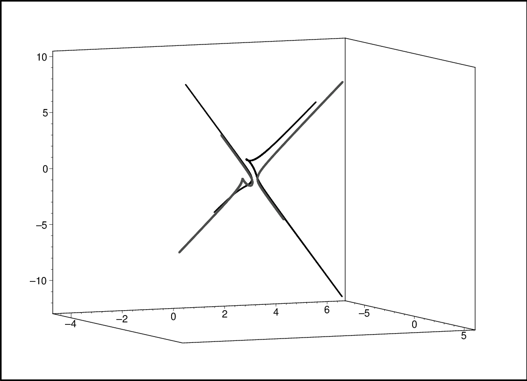
It only remains to compute the numerator of the third component of the rational parametrization of the lifted curve; namely p3​(t)p_{3}(t). Applying Lemma 3.2 we get the approximate parametrization (see Fig. 2 𝒫⁡(t)=(p1​(t)q⁡(t),p2​(t)q⁡(t),p3​(t)q⁡(t)){\mathcal{P}}(t)=(\frac{p_{1}(t)}{q(t)},\frac{p_{2}(t)}{q(t)},\frac{p_{3}(t)}{q(t)}) of the space curve 𝒞{\mathcal{C}} (i.e. the parametrization of 𝒞¯\overline{{\mathcal{C}}}), where

p3​(t)q⁡(t)=−1.067157288​t3−0.2783759249−0.7182447737​t+1.955832944​t2−0.9059858774+1.956830479​t−0.6103552658​t2−1.494650450​t3+t4.\frac{p_{3}(t)}{q(t)}={\frac{-1.067157288\,{t}^{3}-0.2783759249-0.7182447737\,t+1.955832944\,{t}^{2}}{-0.9059858774+1.956830479\,t-0.6103552658\,{t}^{2}-1.494650450\,{t}^{3}+{t}^{4}}}.

Refer to caption

Figure 2: Joint plot of 𝒞{\mathcal{C}} and 𝒞¯\overline{{\mathcal{C}}}
Example 4.3.

Let 𝒞{\mathcal{C}} be the space curve defined by the polynomials

F1=\displaystyle\mathit{F_{1}}= 20052827033​x​y+2850904342​z​y−7155364672​z​x−215763180597100​x\displaystyle 20052827033xy+2850904342zy-7155364672zx-\frac{215763180597}{100}x
−7869010116​z+1743412651801100​y−43102722226​y2+1610946062​z2\displaystyle-7869010116z+\frac{1743412651801}{100}y-43102722226y^{2}+1610946062z^{2}
F2=\displaystyle\mathit{F_{2}}= −18330943984​z​y+33857630124​z​x−39018840299925​x−56921602320​z+\displaystyle-18330943984zy+33857630124zx-\frac{390188402999}{25}x-56921602320z+
12611223036001100​y−166608514760​y2+57179742076​z2+20052827033​x2\displaystyle\frac{12611223036001}{100}y-166608514760y^{2}+57179742076z^{2}+20052827033x^{2}

and let ϵ=1600\epsilon=\frac{1}{600}. One can check that 𝒞{\mathcal{C}} satisfies all the hypotheses imposed in Section 1. Moreover, deg⁡(𝒞)=4{\rm deg}({\mathcal{C}})=4. The projected curve πz​(𝒞)∗\pi_{z}({\mathcal{C}})^{*} is not ϵ\epsilon-rational, but πy​(𝒞)\pi_{y}({\mathcal{C}}) is. So we work with the projection on the plane y=0y=0. The defining polynomial of πy​(𝒞)∗\pi_{y}({\mathcal{C}})^{*} is

f⁡(x,z)=6.959832072⋅1047​z​x−4.075715387⋅1036​x−6.207866771⋅1035​z+1.769623619⋅1047​x3+9.541705261⋅1046​x2+1.269145848⋅1048​z2+8.077561390⋅1047​x3​z−1.355904241⋅1048​x2​z−2.573514563⋅1048​z3+2.289865008⋅1048​z4−3.292700550⋅1048​z2​x+4.798217962⋅1048​x​z3+3.090311649⋅1048​x2​z2−2.981944666⋅1047​x4.f(x,z)={6.959832072\cdot 10^{47}}\,zx-{4.075715387\cdot 10^{36}}\,x-{6.207866771\cdot 10^{35}}\,z+{1.769623619\cdot 10^{47}}\,{x}^{3}+{9.541705261\cdot 10^{46}}\,{x}^{2}+{1.269145848\cdot 10^{48}}\,{z}^{2}+{8.077561390\cdot 10^{47}}\,{x}^{3}z-{1.355904241\cdot 10^{48}}\,{x}^{2}z-{2.573514563\cdot 10^{48}}\,{z}^{3}+{2.289865008\cdot 10^{48}}\,{z}^{4}-{3.292700550\cdot 10^{48}}\,{z}^{2}x+{4.798217962\cdot 10^{48}}\,x{z}^{3}+{3.090311649\cdot 10^{48}}\,{x}^{2}{z}^{2}-{2.981944666\cdot 10^{47}}\,{x}^{4}.

Note that deg⁡(πy​(𝒞)∗)=4{\rm deg}(\pi_{y}({\mathcal{C}})^{*})=4. Applying the approximate parametrization algorithm for plane curves in [20] we get that πy​(𝒞)∗\pi_{y}({\mathcal{C}})^{*} is ϵ\epsilon-rational. Furthermore the algorithm outputs 𝒬⁡(t)=(p1​(t)q⁡(t),p3​(t)q⁡(t)){\mathcal{Q}}(t)=(\frac{p_{1}(t)}{q(t)},\frac{p_{3}(t)}{q(t)})

p1=\displaystyle p_{1}= −0.8393730698​t−1.927074242​t2−0.1348623847−0.7172362732​t4−1.9338152490​t3,\displaystyle-0.8393730698t-1.927074242t^{2}-0.1348623847-0.7172362732t^{4}-1.9338152490t^{3},
p3=\displaystyle p_{3}= 0.009163725887​t−0.08721680470​t3+0.004664930306−0.05315337574​t4\displaystyle 0.009163725887t-0.08721680470t^{3}+0.004664930306-0.05315337574t^{4}
−0.03060855191​t2,\displaystyle-0.03060855191t^{2},
q=\displaystyle q= 3.555348439​t3+t4+4.622830832​t2+2.625458073​t+0.5529230644.\displaystyle 3.555348439\,{t}^{3}+{t}^{4}+4.622830832\,{t}^{2}+2.625458073\,t+0.5529230644.

It only remains to compute the numerator of the second component of the rational parametrization of the lifted curve; namely p2​(t)p_{2}(t). Applying Algorithm-Lift we get the parametrization 𝒫⁡(t)=(p1​(t)q⁡(t),p2​(t)q⁡(t),p3​(t)q⁡(t)){\mathcal{P}}(t)=(\frac{p_{1}(t)}{q(t)},\frac{p_{2}(t)}{q(t)},\frac{p_{3}(t)}{q(t)}) of the space curve 𝒞¯\overline{\mathcal{C}} where

p2=\displaystyle p_{2}= 0.3088642466​t+0.4323589964​t2+0.07398086924+0.2023592378​t3.\displaystyle 0.3088642466t+0.4323589964t^{2}+0.07398086924+0.2023592378t^{3}.

5 Error Analysis

In this section, we prove that the Hausdorff distance between the input and output curves, of our algorithm, is always finite. For this purpose, we first need to develop some results on asymptotes of space curves. Afterwards we will analyze the distance. To start, we briefly recall the notion of Hausdorff distance; for further details we refer to [1]. In a metric space (X,d)(X,{\rm d}), for ∅≠B⊂X\emptyset\neq B\subset X and a∈Xa\in X we define

d⁡(a,B)=infb∈B​{d⁡(a,b)}.{\rm d}(a,B)={\rm inf}_{b\in B}\{{\rm d}(a,b)\}.

Moreover, for A,B⊂X∖∅A,B\subset X\setminus\emptyset we define

Hd​(A,B)=max⁡{supa∈A​{d⁡(a,B)},supb∈B​{d⁡(b,A)}}.{\rm H}_{\rm d}(A,B)=\max\{{\rm sup}_{a\in A}\{{\rm d}(a,B)\},{\rm sup}_{b\in B}\{{\rm d}(b,A)\}\}.

By convention Hd​(∅,∅)=0{\rm H}_{\rm d}(\emptyset,\emptyset)=0 and, for ∅≠A⊂X\emptyset\neq A\subset X, Hd​(A,∅)=∞{\rm H}_{\rm d}(A,\emptyset)=\infty. The function Hd{\rm H}_{\rm d} is called the Hausdorff distance induced by d{\rm d}. In our case, since we will be working in (ℂ3,d)({\mathbb{C}}^{3},{\rm d}) or (ℝ3,d)({\mathbb{R}}^{3},{\rm d}), being d{\rm d} the usual unitary or Euclidean distance, we simplify the notation writing H⁡(A,B){\rm H}(A,B).

Let ℰ{\mathcal{E}} be an space curve in ℂ3{\mathbb{C}}^{3}; similarly if we consider the curve in ℂn{\mathbb{C}}^{n}. The intuitive idea of asymptote is clear, but here we formalize it and state some results. Although these results might be part of the background on the theory of asymptotes, we have not been able to find a reference in the literature suitable for our needs.

We say that a line ℒ\cal L in ℂ3{\mathbb{C}}^{3} is an asymptote of ℰ{\mathcal{E}} if there exists a sequence {Pn}n∈ℕ\{P_{n}\}_{n\in\mathbb{N}} of points in ℰ{\mathcal{E}} such that limn​‖Pn‖=∞{\rm lim}_{n}\|P_{n}\|=\infty and limn​d​(Pn,ℒ)=0{\rm lim}_{n}{\rm d}(P_{n},{\cal L})=0; where dd denotes the usual unitary distance in ℂ3{\mathbb{C}}^{3} and ∥⁣∥\|\,\| the associated norm. In the following, we show how the tangents at the simple points at infinity of ℰ{\mathcal{E}} are related with the asymptotes. More precisely, we have the following lemma. In the sequel, if 𝒱\cal V is a projective variety in ℙ3​(𝔽){\mathbb{P}}^{3}({\mathbb{F}}), we denote by 𝒱a{\cal V}_{a} the open set 𝒱∩{w≠0}{\cal V}\cap\{w\neq 0\}. In addition, for λ∈ℂ\lambda\in{\mathbb{C}}, λ¯\overline{\lambda} denotes its conjugate.

Lemma 5.1.

Let P=(a:b:c:0)∈ℰ∞P=(a:b:c:0)\in{\mathcal{E}}^{\infty} be simple and let 𝕋⁡(P,ℰh)\mathbb{T}(P,{\mathcal{E}}^{h}) be the tangent line to ℰh{\mathcal{E}}^{h} at PP. If 𝕋⁡(P,ℰh)\mathbb{T}(P,{\mathcal{E}}^{h}) is not included in the plane w=0w=0, then 𝕋​(P,ℰh)a\mathbb{T}(P,{\mathcal{E}}^{h})_{a} is an asymptote of ℰ{\mathcal{E}}. Moreover, (a¯,b¯,c¯)(\overline{a},\overline{b},\overline{c}) is a direction vector of the asymptote.

Proof. Let {H1,…,Hm}⊂𝔽⁡[x,y,z,w]\{H_{1},\ldots,H_{m}\}\subset{\mathbb{F}}[x,y,z,w] be homogeneous polynomials defining the ideal of ℰh{\mathcal{E}}^{h}. Let

πi​(x,y,z,w)=∂Hi∂x​(P)​x+∂Hi∂y​(P)​y+∂Hi∂z​(P)​z+∂Hi∂w​(P)​w.\pi_{i}(x,y,z,w)=\frac{\partial H_{i}}{\partial x}(P)x+\frac{\partial H_{i}}{\partial y}(P)y+\frac{\partial H_{i}}{\partial z}(P)z+\frac{\partial H_{i}}{\partial w}(P)w.

Then, 𝕋⁡(P,ℰh)\mathbb{T}(P,{\mathcal{E}}^{h}) is the projective variety defined by {π1​(x,y,z,w),…,πm​(x,y,z,w)}\{\pi_{1}(x,y,z,w),\ldots,\pi_{m}(x,y,z,w)\} (see e.g. pp. 181 in [13]). Note that, since 𝕋⁡(P,ℰh)\mathbb{T}(P,{\mathcal{E}}^{h}) is not included in the plane w=0w=0, 𝕋​(P,ℰh)a\mathbb{T}(P,{\mathcal{E}}^{h})_{a} is an affine line. Now, we consider a local parametrization 𝒫(t)=(x~(t):y~(t):z~(t):w(t)){\mathcal{P}}(t)=(\tilde{x}(t):\tilde{y}(t):\tilde{z}(t):w(t)) of ℰh{\mathcal{E}}^{h} centered at PP. Since PP is simple, and its tangent is not included in w=0w=0, the multiplicity of intersection of ℰh{\mathcal{E}}^{h} and the plane w=0w=0 at PP is 1. Thus, w⁡(t)w(t) can be expressed as w⁡(t)=t​u​(t)w(t)=tu(t), where u⁡(t)u(t) has order 0. Therefore, u​(t)−1u(t)^{-1} is a power series and 𝒫⁡(t){\mathcal{P}}(t) can be expressed as

𝒫(t)=(x(t):y(t):z(t):t){\mathcal{P}}(t)=(x(t):y(t):z(t):t)

where x⁡(t)=x~​(t)​u−1​(t)x(t)=\tilde{x}(t)u^{-1}(t), y⁡(t)=y~​(t)​u−1​(t)y(t)=\tilde{y}(t)u^{-1}(t), z⁡(t)=z~​(t)​u−1​(t)z(t)=\tilde{z}(t)u^{-1}(t) are power series. Moreover, since 𝕋⁡(P,ℰh)\mathbb{T}(P,{\mathcal{E}}^{h}) is the tangent, the order of πi​(𝒫​(t))\pi_{i}({\mathcal{P}}(t)) has to be, at least, 2. Therefore, πi​(𝒫​(t))\pi_{i}({\mathcal{P}}(t)) can be expressed as πi​(𝒫⁡(t))=tℓi​v​(t),\pi_{i}({\mathcal{P}}(t))=t^{\ell_{i}}v(t), where ℓi>1\ell_{i}>1 and v⁡(t)v(t) has order 0.

Now, let {tn}\{t_{n}\} be a sequence of complex numbers converging to 00, and such that tn≠0t_{n}\neq 0. Then, for all nn, Pn=(x⁡(tn)tn,y⁡(tn)tn,z⁡(tn)tn)∈ℰP_{n}=(\frac{x(t_{n})}{t_{n}},\frac{y(t_{n})}{t_{n}},\frac{z(t_{n})}{t_{n}})\in{\mathcal{E}}. Moreover, limn​‖Pn‖=∞{\rm lim}_{n}\|P_{n}\|=\infty. Let Πi\Pi_{i} be the affine plane defined by πi​(x,y,z,1)\pi_{i}(x,y,z,1). We prove that, for all ii, limn​d​(Pn,Πi)=0{\rm lim}_{n}{\rm d}(P_{n},\Pi_{i})=0. From where, one deduces that limn​d​(Pn,𝕋​(P,ℰh)a)=0{\rm lim}_{n}{\rm d}(P_{n},\mathbb{T}(P,{\mathcal{E}}^{h})_{a})=0, and hence that 𝕋​(P,ℰh)a\mathbb{T}(P,{\mathcal{E}}^{h})_{a} is an asymptote.

Indeed,

d⁡(Pn,Πi)=|πi​(Pn,1)|‖(∂Hi∂x​(P),∂Hi∂y​(P),∂Hi∂z​(P))‖=|tnℓi−1​v​(tn)|‖(∂Hi∂x​(P),∂Hi∂y​(P),∂Hi∂z​(P))‖.{\rm d}(P_{n},\Pi_{i})=\frac{\left|\pi_{i}(P_{n},1)\right|}{\left\|\left(\frac{\partial H_{i}}{\partial x}(P),\frac{\partial H_{i}}{\partial y}(P),\frac{\partial H_{i}}{\partial z}(P)\right)\right\|}=\frac{\left|t_{n}^{\ell_{i}-1}v(t_{n})\right|}{\left\|\left(\frac{\partial H_{i}}{\partial x}(P),\frac{\partial H_{i}}{\partial y}(P),\frac{\partial H_{i}}{\partial z}(P)\right)\right\|}.

Since the denominator is not zero, because 𝕋⁡(P,ℰh)\mathbb{T}(P,{\mathcal{E}}^{h}) is not included in w=0w=0, and since ℓi−1>0\ell_{i}-1>0 and order of vv is 0, we get that limn​d​(Pn,Πi)=0{\rm lim}_{n}{\rm d}(P_{n},\Pi_{i})=0.

Finally, we see that u=(a¯,b¯,c¯)u=(\overline{a},\overline{b},\overline{c}) is a direction vector of the asymptote. First we observe that uu is not zero, since P∈ℙ3​(𝔽)P\in{P}^{3}({\mathbb{F}}). Now, by Euler equality we have that

∂Hi∂x​x+∂Hi∂y​y+∂Hi∂z​z+∂Hi∂w​w=deg⁡(Hi)​Hi.\frac{\partial H_{i}}{\partial x}x+\frac{\partial H_{i}}{\partial y}y+\frac{\partial H_{i}}{\partial z}z+\frac{\partial H_{i}}{\partial w}w={\rm deg}(H_{i})H_{i}.

Substituting by PP, we get

∂Hi∂x​(P)​a+∂Hi∂y​(P)​b+∂Hi∂z​(P)​c+∂Hi∂w​(P)​0=deg⁡(Hi)​Hi​(P)=0.\frac{\partial H_{i}}{\partial x}(P)a+\frac{\partial H_{i}}{\partial y}(P)b+\frac{\partial H_{i}}{\partial z}(P)c+\frac{\partial H_{i}}{\partial w}(P)0={\rm deg}(H_{i})H_{i}(P)=0.

Hence,

(∂Hi∂x​(P),∂Hi∂y​(P),∂Hi∂z​(P))⋅u=∂Hi∂x​(P)​a+∂Hi∂y​(P)​b+∂Hi∂z​(P)​c=0.\left(\frac{\partial H_{i}}{\partial x}(P),\frac{\partial H_{i}}{\partial y}(P),\frac{\partial H_{i}}{\partial z}(P)\right)\cdot u=\frac{\partial H_{i}}{\partial x}(P)a+\frac{\partial H_{i}}{\partial y}(P)b+\frac{\partial H_{i}}{\partial z}(P)c=0.

Thus uu is orthogonal to all the planes Πi\Pi_{i}.

Remark 5.2.

Given PP verifying the conditions of Lemma 5.1, we observe that:

  1. 1.

    The asymptote determined by PP can only be real if PP is real. This is due to the fact that ℰh{\mathcal{E}}^{h} is defined by real polynomials

  2. 2.

    If the real asymptote ℒ\cal L determined by PP is real, then there exists a real branch of ℰ{\mathcal{E}} approaching ℒ\cal L in each of the two directions of ℒ\cal L. Indeed let 𝒫(t)=(x(t):y(t):z(t):t){\mathcal{P}}(t)=(x(t):y(t):z(t):t) be, as in the proof of Lemma 5.1, a real local parametrization centered at PP. x⁡(t),y⁡(t),z⁡(t)x(t),y(t),z(t) are power series and at least one of them (say w.l.o.g. x⁡(t)x(t)) is of order 00. Thus the affine branch tending to PP is locally parametrized by 𝒫a​(t)=1t​(x⁡(t),y⁡(t),z⁡(t)){\mathcal{P}}^{a}(t)=\frac{1}{t}(x(t),y(t),z(t)). Therefore,

    x⁡(t)t=a0+a1​t+a2​t2+⋯t=a0t+a1+t⁡(a2+⋯)​with​a=a0≠0.\frac{x(t)}{t}=\frac{a_{0}+a_{1}t+a_{2}t^{2}+\cdots}{t}=\frac{a_{0}}{t}+a_{1}+t(a_{2}+\cdots)\,\,\,\mbox{with}\,\,a=a_{0}\neq 0.

    Let us assume w.l.o.g. that a0>0a_{0}>0. On the other hand limt→0​x⁡(t)t=∞{\rm lim}_{t\rightarrow 0}\frac{x(t)}{t}=\infty. Therefore, for positive values t+t^{+} of tt, sufficiently close to 00, the first coordinate of 𝒫a​(t+){\mathcal{P}}^{a}(t^{+}) is positive, while for negative values t−t^{-} of tt, sufficiently close to 00, the first coordinate of 𝒫a​(t−){\mathcal{P}}^{a}(t^{-}) is negative. Thus, the real branch is approaching infinity following both directions of the asymptote.

  3. 3.

    Let all points in ℰ∞{\mathcal{E}}^{\infty} satisfy the conditions of Lemma 5.1. Then, ℰ∩ℝ3{\mathcal{E}}\cap{\mathbb{R}}^{3} is unbounded iff there is at least one real point in ℰ∞{\mathcal{E}}^{\infty}.

Lemma 5.3.

Let ℰ1,ℰ2⊂ℂ3{\mathcal{E}}_{1},{\mathcal{E}}_{2}\subset{\mathbb{C}}^{3} be irreducible real curves such that ℰ1∞=ℰ2∞{\mathcal{E}}_{1}^{\infty}={\mathcal{E}}_{2}^{\infty} and card⁡(ℰ1∞)=card⁡(ℰ2∞)=deg⁡(ℰ1)=deg⁡(ℰ2){\rm card}({\mathcal{E}}_{1}^{\infty})={\rm card}({\mathcal{E}}_{2}^{\infty})={\rm deg}({\mathcal{E}}_{1})={\rm deg}({\mathcal{E}}_{2}). Then,

  1. 1.

    ℰi{\mathcal{E}}_{i} has deg⁡(ℰi){\rm deg}({\mathcal{E}}_{i}) different asymptotes, non of them parallel.

  2. 2.

    For each asymptote ℒ\cal L of ℰ1{\mathcal{E}}_{1} there exists exactly one asymptote ℒ¯\overline{\cal L} of ℰ2{\mathcal{E}}_{2} such that ℒ{\cal L} and ℒ¯\overline{\cal L} are parallel.

  3. 3.

    For each real asymptote ℒ\cal L of ℰ1{\mathcal{E}}_{1} there exists exactly one real asymptote ℒ¯\overline{\cal L} of ℰ2{\mathcal{E}}_{2} such that ℒ{\cal L} and ℒ¯\overline{\cal L} are parallel.

Proof. Let d=deg⁡(ℰ1)=deg⁡(ℰ2)d={\rm deg}({\mathcal{E}}_{1})={\rm deg}({\mathcal{E}}_{2}). Since all points at infinity of both curves are simple and no tangent line is included in the plane at infinity, Lemma 5.1 implies that each curve has exactly dd asymptotes. Furthermore, since card⁡(ℰi∞)=d{\rm card}({\mathcal{E}}_{i}^{\infty})=d, again by Lemma 5.1, the direction vectors are different and not parallel. This proves (1). (2) follows from (1) and ℰ1∞=ℰ2∞{\mathcal{E}}_{1}^{\infty}={\mathcal{E}}_{2}^{\infty}. (3) follows from (2) and Remark 5.2 (1).

Applying the previous lemmas we get the next theorem.

Theorem 5.4.

Let ℰ1,ℰ2⊂ℂ3{\mathcal{E}}_{1},{\mathcal{E}}_{2}\subset{\mathbb{C}}^{3} be irreducible real curves such that ℰ1∞=ℰ2∞{\mathcal{E}}_{1}^{\infty}={\mathcal{E}}_{2}^{\infty} and card⁡(ℰ1∞)=card⁡(ℰ2∞)=deg⁡(ℰ1)=deg⁡(ℰ2){\rm card}({\mathcal{E}}_{1}^{\infty})={\rm card}({\mathcal{E}}_{2}^{\infty})={\rm deg}({\mathcal{E}}_{1})={\rm deg}({\mathcal{E}}_{2}). Then, H⁡(ℰ1∩ℝ3,ℰ2∩ℝ3)<∞{\rm H}({\mathcal{E}}_{1}\cap{\mathbb{R}}^{3},{\mathcal{E}}_{2}\cap{\mathbb{R}}^{3})<\infty.

Proof. By Remark 5.2 (3), ℰ1∩ℝ3{\mathcal{E}}_{1}\cap{\mathbb{R}}^{3} is bounded iff ℰ2∩ℝ3{\mathcal{E}}_{2}\cap{\mathbb{R}}^{3} is bounded. Moreover, if both are bounded the result follows from Lemma 3.58 in [1]. If they are not bounded, let ℒ1,…,ℒn{\cal L}_{1},\ldots,{\cal L}_{n} be the real asymptotes of ℰ1{\mathcal{E}}_{1} and let ℒ¯∞,…,ℒ¯\\overline{\cal L}_{1},\ldots,\overline{\cal L}_{n} be the real asymptotes of ℰ2{\mathcal{E}}_{2}, with ℒi∥ℒ¯⟩{\cal L}_{i}\parallel\overline{\cal L}_{i}; see Lemma 5.3. In addition let δi\delta_{i} be the real branch of ℰ1{\mathcal{E}}_{1} approaching the asymptote ℒi{\cal L}_{i}; similarly for δ¯i\overline{\delta}_{i} and ℒ¯⟩\overline{\cal L}_{i}. Let γ=max{H(ℒi,ℒ¯⟩)|⟩=∞,…,\}\gamma=\max\{{\rm H}({\cal L}_{i},\overline{\cal L}_{i})\,|\,i=1,\ldots,n\}; by Lemma 3.58, in [1], γ∈ℝ\gamma\in{\mathbb{R}}. Now, let ρ>0\rho>0, and consider the cylinder ViV_{i} around ℒi{\cal L}_{i} at distance ρ\rho; similarly V¯i\overline{V}_{i} is the cylinder around ℒ¯⟩\overline{\cal L}_{i} at distance ρ\rho.

Let us see that ℰ1⊈(V1∪⋯∪Vn){\mathcal{E}}_{1}\nsubseteq(V_{1}\cup\cdots\cup V_{n}). If ℰ1{\mathcal{E}}_{1} was included, since ℰ1{\mathcal{E}}_{1} is irreducible then it would be included in one ViV_{i}; say in V1V_{1}. Then, for every sequence {Pn}n∈ℕ\{P_{n}\}_{n\in{\mathbb{N}}} of points of ℰ1{\mathcal{E}}_{1} such that limn​‖Pn‖2=∞{\rm lim}_{n}\|P_{n}\|_{2}=\infty, one has that limn​d​(Pn,ℒ1)=ρ>0{\rm lim}_{n}{\rm d}(P_{n},{\cal L}_{1})=\rho>0 and limn​d​(Pn,ℒj)=∞{\rm lim}_{n}{\rm d}(P_{n},{\cal L}_{j})=\infty for j≠1j\neq 1 (note that ℒ1​|ℒj{\cal L}_{1}\not\,\parallel{\cal L}_{j} if j>1j>1). Thus, ℰ1{\mathcal{E}}_{1} would have no asymptote. Similarly, one has that ℰ2⊈(V¯1∪⋯∪V¯n){\mathcal{E}}_{2}\nsubseteq(\overline{V}_{1}\cup\cdots\cup\overline{V}_{n}).

Let Δ1=ℰ1∩(V1∪⋯∪Vn)\Delta_{1}={\mathcal{E}}_{1}\cap(V_{1}\cup\cdots\cup V_{n}) and Δ2=ℰ2∩(V¯1∪⋯∪V¯n)\Delta_{2}={\mathcal{E}}_{2}\cap(\overline{V}_{1}\cup\cdots\cup\overline{V}_{n}). Because of the reasoning above card⁡(Δ1∪Δ2)<∞{\rm card}(\Delta_{1}\cup\Delta_{2})<\infty. So, let α=max⁡{‖P‖2|P∈Δ1∪Δ2}\alpha=\max\{\|P\|_{2}\,|\,P\in\Delta_{1}\cup\Delta_{2}\}. In this situation, we can choose a compact ball BB centered at the origin, and with a sufficiently big radius (and bigger than α\alpha) such that (ℰ1∪ℰ2)∩ℝ3({\mathcal{E}}_{1}\cup{\mathcal{E}}_{2})\cap{\mathbb{R}}^{3} is included in BB union the inner part of the cylinders V1,…,Vn,V¯1,…,V¯nV_{1},\ldots,V_{n},\overline{V}_{1},\ldots,\overline{V}_{n}. Now, let P∈ℰ1∩ℝ3P\in{\mathcal{E}}_{1}\cap{\mathbb{R}}^{3}, then

  • •

    If P∈BP\in B then d⁡(P,ℰ2∩ℝ3)≤d⁡(P,ℰ2∩ℝ3∩B)≤H⁡(ℰ1∩ℝ3∩B,ℰ2∩ℝ3∩B){\rm d}(P,{\mathcal{E}}_{2}\cap{\mathbb{R}}^{3})\leq{\rm d}(P,{\mathcal{E}}_{2}\cap{\mathbb{R}}^{3}\cap B)\leq{\rm H}({\mathcal{E}}_{1}\cap{\mathbb{R}}^{3}\cap B,{\mathcal{E}}_{2}\cap{\mathbb{R}}^{3}\cap B) that is equal to a real number MM, because of Lemma 3.58 in [1].

  • •

    If P∉BP\not\in B then PP is included in the interior of one of the cylinders ViV_{i}. Say PP is in the interior of V1V_{1}; so P∈δ1P\in\delta_{1}. By Remark 5.2 (2), we know that in δ1\delta_{1} we can distinguish two branches each in each direction of the asymptote, let us call them δ1+\delta_{1}^{+} and δ1−\delta_{1}^{-}, and say that P∈δ1+P\in\delta_{1}^{+}; similarly for δ¯1,δ¯1+,δ¯1−\overline{\delta}_{1},\overline{\delta}_{1}^{+},\overline{\delta}_{1}^{-}. In this situation, there exist A∈ℒ1,B∈ℒ¯∞A\in{\cal L}_{1},B\in\overline{\cal L}_{1} and Q∈δ¯1+∩(ℝ3∖B)Q\in\overline{\delta}_{1}^{+}\cap({\mathbb{R}}^{3}\setminus B) such that

    d⁡(P,A)≤ρ,d⁡(A,B)≤γ,d⁡(B,Q)≤ρ.{\rm d}(P,A)\leq\rho,{\rm d}(A,B)\leq\gamma,{\rm d}(B,Q)\leq\rho.

    Therefore, d⁡(P,Q)≤2​ρ+γ{\rm d}(P,Q)\leq 2\rho+\gamma. That is, for every P∈ℰ1∩(ℝ3∖B)P\in{\mathcal{E}}_{1}\cap({\mathbb{R}}^{3}\setminus B) there exists Q∈ℰ2∩ℝ3Q\in{\mathcal{E}}_{2}\cap{\mathbb{R}}^{3} such that d⁡(P,Q)<2​ρ+γ{\rm d}(P,Q)<2\rho+\gamma; so d⁡(P,ℰ2∩ℝ3)<2​ρ+γ{\rm d}(P,{\mathcal{E}}_{2}\cap{\mathbb{R}}^{3})<2\rho+\gamma.

Since the reasoning above can be done analogously for Q∈ℰ2∩ℝ3Q\in{\mathcal{E}}_{2}\cap{\mathbb{R}}^{3}, we conclude that

H⁡(ℰ1∩ℝ3,ℰ2∩ℝ3)≤max⁡{M,2​ρ+γ}.{\rm H}({\mathcal{E}}_{1}\cap{\mathbb{R}}^{3},{\mathcal{E}}_{2}\cap{\mathbb{R}}^{3})\leq\max\{M,2\rho+\gamma\}.
Corollary 5.5.

Let 𝒞,𝒞¯{\mathcal{C}},\overline{\mathcal{C}} be the input and output curves of our algorithm. Then H⁡(𝒞∩ℝ3,𝒞¯∩ℝ3)<∞{\rm H}({\mathcal{C}}\cap{\mathbb{R}}^{3},\overline{\mathcal{C}}\cap{\mathbb{R}}^{3})<\infty.

Proof. It follows from the general assumptions, and from Theorems 3.1 and 5.4.

References

  • [1] Aliprantis C.D., Border K.C. (2006). Infinite Dimensional Analysis. Springer Verlag (2006).
  • [2] Bajaj C., Royappa A., (2000). Parameterization In Finite Precision. Algorithmica, Vol. 27, No. 1. pp. 100-114.
  • [3] Caviness B.F, Johnson J.R. (1998). Quantifier Elimination and Cylindrical Algebraic Decomposition. Text and Monographs in Symbolic Computation. Springer Verlag, pp 269–289.
  • [4] Corless R.M., Gianni P.M., Trager B.M., Watt S.M. (1995). The Singular Value Decomposition for Polynomial Systems. Proc. ISSAC 1995, pp. 195-207, ACM Press.
  • [5] Gianni P., Trager B., and Zacharias G. (1988). Grobner bases and primary decompositions of polynomial ideals. Journal of Symbolic Computation, Vol. 6, pp. 149-167.
  • [6] Corless R.M., Giesbrecht M.W., Kotsireas I.S., van Hoeij M., Watt S.M. (2001). Towards Factoring Bivariate Approximate Polynomials. Proc. ISSAC 2001, London, Bernard Mourrain, ed. pp 85–92.
  • [7] Corless R.M., Giesbrecht M.W., Kotsireas I.S., Watt S.M. (2000). Numerical Implicitization of Parametric Hypersurfaces with Linear Algebra. Proc. Artificial Intelligence with Symbolic Computation (AISC 2000), pp 174-183, Springer Verlag LNAI 1930.
  • [8] Cox D., Little J., O’Shea D. (1997). Ideals, Varieties, and Algorithms (2nd ed.). Springer-Verlag, New York.
  • [9] Dokken T., (2001). Approximate Implicitization. Mathematical Methods in CAGD;Oslo 2000, Tom Lyche anf Larry L. Schumakes (eds). Vanderbilt University Press.
  • [10] Emiris I.Z., Galligo A., Lombardi H., (1997). Certified Approximate Univariate GCDs J. Pure and Applied Algebra, Vol.117 and 118. pp. 229–251.
  • [11] Gahleitner J., Jüttler B., Schicho J. (2002). Approximate Parameterization of Planar Cubic Curve Segments. Proc. Fifth International Conference on Curves and Surfaces. Saint-Malo 2002. pp. 1-13, Nashboro Press, Nashville, TN.
  • [12] Galligo A., Rupprech D. (2002). Irreducible Decomposition of Curves. J. Symbolic Computation, Vol. 33. pp. 661 - 677.
  • [13] Harris J. (1992). Algebraic Geometry, a First Course. Springer-Verlag.
  • [14] Hartmann E., (2000). Numerical Parameterization of Curves and Surfaces. Computer Aided Geometry Design, Vol. 17. pp. 251-266.
  • [15] Kaltofen E., May J.P., Yang Z., Zhi L., (2008). Approximate Factorization of Multivariate Polynomials Using Singular Value Decomposition. Journal of Symbolic Computation. Vol.43/5. pp.359-376.
  • [16] Pan V.Y., (1996). Numerical Computation of a Polynomial GCD and Extensions. Tech.report, N. 2969. Sophia-Antipolis, France.
  • [17] Pérez–Díaz S., Sendra J., Sendra J.R., (2004). Parametrization of Approximate Algebraic Curves by Lines. Theoretical Computer Science. Vol.315/2-3. pp.627-650.
  • [18] Pérez–Díaz S., Sendra J., Sendra J.R., (2005). Parametrization of Approximate Algebraic Surfaces by Lines. Computer Aided Geometric Design. Vol 22/2. pp. 147-181.
  • [19] Pérez–Díaz S., Sendra J., Sendra J.R., (2006). Distance Bounds of ϵ\epsilon-Points on Hypersurfaces. Theoretical Computer Science. Vol. 359, pp. 344-368.
  • [20] Pérez–Díaz S., Rueda S.L., Sendra J., Sendra J.R., (2010). Approximate Parametrization of Plane Algebraic Curves by Linear Systems of Curves. Computer Aided Geometric Design vol 27, 212–231.
  • [21] Robbiano L, J. Abbott J. (ed) (2010). ApCoA = Embedding Commutative Algebra into Analysis. In Approximate Commutative Algebra Texts and Monographs in Symbolic Computation. Springer-Velag.
  • [22] Sendra J.R., Winkler J.R., Pérez-Díaz S. (2007). Rational Algebraic Curves: A Computer Algebra Approach. Springer-Verlag Heidelberg, in series Algorithms and Computation in Mathematics. Volume 22.
  • [23] Stetter H.J. (2004). Numerical Polynomial Algebra. SIAM.
  • [24] Stetter H.J. (2010). ApCoA = Embedding Commutative Algebra into Analysis. In [21] pp. 205-217
  • [25] Winkler F., (1996). Polynomial Algorithms in Computer Algebra. Springer-Verlag, Wien New York.