Dark goo: Bulk viscosity as an alternative to dark energy

The background equations 2 and 3 are effective equations that do not rely on microscopic physics, except through the bulk viscosity parameter. We thus need some microscopic physics to “personify” the bulk viscosity. For reasons we discuss in section 2.3, no Standard Model particles can produce a bulk viscosity in the late universe. We thus need to add a new component to the energy content of the universe in order to induce some bulk viscosity in the present universe.

For simplicity, we add a massive scalar field with quartic interactions to the Lagrangian of the Standard Model (cubic interactions would change our results in a trivial way and are left out in the following):

We also make several assumptions. First we require that the assumptions of hydrodynamics for this scalar fluid are satisfied. The validity of hydrodynamics is crucial for the concept of bulk viscosity to make sense. These assumptions include local thermal equilibrium, small inhomogeneities (gradients) and absence of instabilities. Each of these points are discussed in section 2.3. We also assume that the scalar and Standard Model particles are in thermal equilibrium in the early universe and decouple from each other afterward. After this decoupling time, the temperature of the self-interacting scalars has a distinct evolution from that of photons and other Standard Model particles in equilibrium with the photons. Between electron-positron annihilation and today, the photon temperature scales as $T_{\gamma}\propto a^{-1}$. We shall see later that the scalar temperature $T_{s}$ scales in the same way at least between the time of scalar-photon decoupling and the non-relativistic transition ($T_{s}\sim m_{0}$). Hence, the ratio $T_{s}/T_{\gamma}$ is expected to remain constant over a long time interval, typically from Big Bang Nucleosynthesis until the end of radiation domination.

The model has three free parameters: the mass $m_{0}$, the self-coupling $\lambda$ of the scalar particles, and the ratio of scalar to photon temperatures $\epsilon=T_{s}/T_{\gamma}$ after electron-positron annihilation. Note that $\epsilon\leq 1$ because $(aT_{\gamma})$ can increase due entropy releases until electron-positron annihilation, while $(aT_{s})$ stays constant (no interaction with the Standard Model particles) after scalar-photon decoupling. The limit $\epsilon=1$ correspond to late decoupling not followed by any entropy release and the limit $\epsilon\ll 1$ corresponds to early decoupling with significant entropy releases.

We stress that our model is very different from quintessence models. Both include a scalar field with a potential, but the range of parameters is different. In quintessence models, the scalar field is seen as classical and coherent over large scales, and the potential is adjusted in such a way as to obtain slow-roll conditions in the late universe. In contrast, we are dealing here with a fluid of scalar particles, and we adjust the parameters of our model in order to allow collective (bulk viscous) effects to play a significant role in this imperfect fluid in the present universe.

We also mention that our model is not a generalization of previous bulk viscous or Chaplygin gas models. The functional form we use for the bulk viscosity (see section 2.2) is very different from the (generalized) Chaplygin form. The bulk viscosity for a scalar theory has been computed from first principles and depends on the physical properties (mass and self-coupling) of the scalar particles; no such interpretation is available for the (generalized) Chaplygin gas form.

We need the pressure, energy density and bulk viscosity of a scalar field to integrate eqs. 2 and 3. The pressure of a gas of massive scalar particles (with vanishing chemical potential) is given by (e.g. Kapusta and Gale ()):

where $K_{2}$ is a modified bessel function of the second kind. In the following we neglect $O(\lambda T_{s}^{4})$ since we expect bulk viscous effect to dominate at low temperature. Using the thermodynamic relation $\rho=T^{2}\partial\left(p/T\right)/\partial T$, we obtain the corresponding energy density:

In a remarkable tour de force, Jeon has computed the leading order bulk viscosity in a scalar theory from diagrammatic methods Jeon (1995). The computation involves the resummation of an infinite number of diagrams and can only be obtained numerically. A best fit of the numerical result is:

where the constants $\kappa_{1}$, $\kappa_{2}$ and $\kappa_{3}$ are 12.13, 1.54 and 1.13, respectively. The thermal mass (i.e. the sum of the zero-temperature mass plus thermal modifications) is given by $m_{\rm th}^{2}=m_{0}^{2}+\delta m_{\rm th}^{2}$, where the thermal modification is $\delta m_{\rm th}^{2}=\lambda T_{s}^{2}/24$. The quantity $\tilde{m}^{2}\equiv m_{\rm th}^{2}-(T_{s}/2)(\partial m_{\rm th}^{2}/\partial T_{s})$ gives the breaking of scale invariance in the theory (at lowest order). More precisely, it is given by $\tilde{m}^{2}=m_{0}^{2}-\beta(\lambda)T_{s}^{2}/48$ where the beta function is $\beta(\lambda)=3\lambda^{2}/(16\pi^{2})$. Note that eq. 9 is only valid for weak coupling $\lambda<1$.

We can understand eq. 9 in the following way. Bulk viscosity characterizes the relaxation of an expanding fluid. As a result, it is proportional to the mean free time between collisions of the fluid constituents. The mean free time is itself inversely proportional to the cross section of the processes responsible for re-establishing equilibrium. In an expanding system, equilibrium is achieved by number changing processes ($2\rightarrow 4$ in $\lambda\phi^{4}$). This explains the $\lambda^{-4}$ dependence of $\zeta$. The exponential is due to Boltzmann suppression of final states for these number changing processes.

The bulk viscosity also vanishes in a conformal theory, since in that case dilatation is a symmetry and the fluid cannot leave equilibrium. It is thus proportional to the (square) of the breaking of scale invariance (i.e. $\tilde{m}^{4}$). Consequently, $\zeta$ has a very different coupling constant behavior at different temperatures. At low temperature $\tilde{m}^{4}\sim m_{0}^{4}$ and $\zeta\sim\lambda^{-4}$; at high temperature $\tilde{m}^{4}\sim\beta^{2}$ and $\zeta\sim\lambda^{(\kappa_{3}-1)/2}$, implying that the bulk viscosity is highly suppressed in this regime.

The crucial point in this model is that the new scalar degree of freedom can be considered as a fluid in the dark energy domination epoch. Otherwise, the concept of bulk viscosity does not make sense. Thus the model must satisfy the assumptions of hydrodynamics. Let’s study each assumption separately.

Local equilibrium.

For a hydrodynamic description to be valid, the fluid constituents must interact sufficiently often so as to maintain (approximate) local equilibrium (the constituents must not be “frozen out”). More technically, the need for local equilibrium is reflected in the fact that transport coefficients are linear deviations away from equilibrium and are computed from equilibrium correlators Jeon (1995).

The criterion to be in equilibrium in an expanding universe is $\Gamma_{\rm scalar}/H\gg 1$, where $\Gamma_{\rm scalar}$ is the rate of processes that are ultimately responsible for the bulk viscosity and $H$ is the expansion rate of the universe. The rate $\Gamma_{\rm scalar}$ is estimated as follows Jeon (1995). First we have that $\Gamma_{\rm scalar}\sim 1/\tau_{\rm free}$ where $\tau_{\rm free}=n/(dW/dVdt)$ is the mean free time between collisions, $n$ is the density of particles and $dW/dVdt$ is the transition rate per unit volume. The processes that are responsible for bulk viscosity in $\lambda\phi^{4}$ theory are $2\rightarrow 4$ scatterings. We expect the bulk viscosity to dominate at low temperature due to the exponential factor in eq. 9. For low temperatures $T\ll m_{0}$ we have $n=dN/dV\sim O(e^{-m_{0}/T_{s}})$ (Boltzmann suppression) and $dW/dVdt\sim O(\lambda^{4}e^{-4m_{0}/T_{s}})$ (there should be a $m_{0}$ to get the units right). Thus the rate of bulk viscosity processes are:

$\displaystyle\Gamma_{\rm scalar}$

$\displaystyle\sim$

$\displaystyle\frac{1}{\tau}\;\;\sim\;\;\frac{m_{0}\lambda^{4}e^{-4m_{0}/T_{s}}}{e^{-m_{0}/T_{s}}}\;\;\sim\;\;m_{0}\lambda^{4}e^{-3m_{0}/T_{s}}.$

(10)

The equilibrium criterion becomes:

$\displaystyle\frac{m_{0}\lambda^{4}e^{-3m_{0}/T_{s}}}{H}\;\;>\;\;1.$

(11)

This criterion must be fulfilled until the present epoch for the model to make sense; this is thus a constraint on the parameters of the model. This also explains why no Standard Model particles produce a large bulk viscosity in the late universe, since they all decouple before dark energy domination.

Small inhomogeneities and gravitational instabilities.

Hydrodynamics is an expansion in gradients (see for example eq. 4). For this expansion to be well defined, velocity gradients must be small (small inhomogeneities). Similarly, clumps of scalar matter may form due to gravity. If these clumps become too large (exponential instabilities), then the fluid breaks apart and a hydrodynamic description is not appropriate anymore.

It is difficult to estimate the size of gradients a priori. For that, a full numerical study of linear perturbations is necessary (a dynamical system analysis might also shed some light on these issues, e.g. Szydlowski and Hrycyna (2007)). We perform such a numerical analysis in section 4. Our results show that linear perturbations are well behaved and no instability develops (see section 4.2).

It is important to emphasize that we are using first order (in gradients) relativistic hydrodynamics. It has been pointed out in Ref. Israel and Stewart (1979) that first order hydrodynamics is acausal and unstable (for certain modes); to cure these problems, second order hydrodynamics should be used instead (see Piattella et al. (2011) for a cosmological case study). A more recent analysis shows that acausality implies unstable behavior Denicol et al. (2008); Pu et al. (2010). The physical explanation is that an acausal disturbance propagating in a light cone would create a singular behavior at the edge of the light cone, since a light cone cannot be crossed in a covariant theory. In our case, growing modes are damped out by bulk viscosity and no instability develops. We conclude that our hydrodynamic equations are well defined and do not produce acausal signal propagation. It thus seems that the use of linear relativistic hydrodynamics is justified for the modes considered here.

Thermodynamical instabilities.

This instability is called “cavitation” (for a discussion, see e.g. Brennen ()). In everyday engineering systems, cavitation manifests itself when the pressure of a fluid goes below its saturated vapor pressure. In such a case, the fluid becomes unstable to the formation of bubbles. The formation of bubbles is akin to the formation of clumps; if there are too many bubbles in the fluid, then a hydrodynamic description is not suitable anymore.

The process of bubble formation is called nucleation. There are two types of nucleation: homogeneous and heterogeneous. Homogeneous nucleation happens when a fluid is pure and smooth. Heterogeneous nucleation happens when a fluid has impurities and is in contact with boundaries.

In our model, the saturated vapor pressure is the vacuum pressure (i.e. zero). Thus when the pressure becomes negative (required for dark energy domination), the fluid becomes in principle unstable to the formation of vacuum bubbles. In the following we use the language of homogeneous nucleation since the fluid is very pure (except maybe for “gravitational” impurities) and smooth (no boundaries).

In everyday engineering systems, it is possible to reduce the pressure of a fluid under its saturated vapor value without forming bubbles (a bit like a supercooled fluid). In other words, a normal fluid can withstand “some” under saturated vapor pressure, it is not automatic that bubbles form. The physics behind that behavior is the following. Under normal conditions, there is formation of voids between the fluid constituents due to thermal fluctuations. When a fluid is subjected to a pressure that is under the saturated vapor pressure, these voids grow and form bubbles. But there is a counter force to this growth due to the potential between fluid constituents. When the outward pressure is greater than the force between constituents, bubbles grow; if not, then the fluid stays as it is. This property of a fluid is called “tensile strength”. For homogeneous nucleation, tensile strength depends only on the properties of the fluid; in heterogeneous nucleation, this tensile strength is strongly dependent on impurities and boundary conditions.

Let’s denote $p_{b\;\rm max}$ the maximum pressure our scalar fluid can sustain without breaking apart (i.e. its tensile strength) and $p_{\rm DE}$ the negative pressure that makes the tiny voids due to thermal fluctuations grow. In the dark energy domination epoch, this pressure is given by $p_{\rm DE}=w\rho_{\rm DE}$, where $w$ is the effective equation of state and $\rho_{\rm DE}\sim 10^{-12}$ eV⁴ is the present dark energy density. A criterion for the absence of cavitation can be phrased in the following way: there is no cavitation in the system if the tensile strength is larger than the maximal outward pressure:

$\displaystyle p_{b\;\rm max}$

$\displaystyle>$

$\displaystyle|w|\rho_{\rm DE}.$

(12)

This condition must be satisfied for a sufficiently long time in order to have dark energy domination without the fluid to break apart. The tensile strength $p_{b\;\rm max}$ is a property of the fluid and may depend on $\lambda$, $m$ and the dimensionless inverse temperature $x=m_{0}/T_{s}$. Thus the above criterion for no cavitation is a constraint on the parameters of the model.

We can roughly estimate the scalar fluid tensile strength using the theory of homogeneous nucleation (e.g. Brennen ()). The result is that the tensile strength is given by:

$\displaystyle p_{b\;\rm max}$

$\displaystyle=$

$\displaystyle\left(\frac{16\pi S^{3}}{3T_{s}\ln(J_{0}/J)}\right)^{1/2},$

(13)

where $S$ is the surface tension and $J$ is the nucleation rate. Since the above relation depends logarithmically on the nucleation rate, we expect a very weak dependence on $J$. Thus for estimate purposes, we set the logarithm to one. The surface tension is a force per unit length; we thus expect it to be proportional to the coupling $\lambda$ and a quantity that has dimensions of [Energy]³. The two relevant energy scales in the problem are $m_{0}$ and $T_{s}$. From dimensional analysis, we obtain four possible forms for the surface tension: $S\sim\lambda T_{s}^{3}$, $S\sim\lambda m_{0}T_{s}^{2}$, $S\sim\lambda m_{0}^{2}T_{s}$ and $S\sim\lambda m_{0}^{3}$. The first one is expected to be valid only at ultra-relativistic energies and we discard it. The last one is unrealistic because of its lack of temperature dependence. Empirical laws show that the typical behavior of surface tension is linear in temperature. We thus use the form $S\sim\lambda m_{0}^{2}T_{s}$ in the following analysis. Plugging $S\sim\lambda m_{0}^{2}T_{s}$ in Eq. (13) we get:

$\displaystyle p_{b\;\rm max}$

$\displaystyle\sim$

$\displaystyle\left(\frac{16\pi}{3}\right)^{1/2}\frac{\lambda^{3/2}m_{0}^{4}}{x}.$

(14)

Combining this with the no cavitation criterion, we obtain the following constraint on the model parameters:

$\displaystyle\frac{\lambda^{3/2}m_{0}^{4}}{x}$

$\displaystyle>$

$\displaystyle\left(\frac{3}{16\pi}\right)^{1/2}|w|\rho_{\rm DE}.$

(15)

Cavitation is also studied in the context of relativistic heavy ion collisions  Rajagopal and Tripuraneni (2010). In this study, it is stated that any hydrodynamic simulations should be stopped when the pressure goes below zero because of cavitation. We argue here that, just like in other engineering systems, a fluid can sustain some negative pressure without cavitating.

The pressure, energy density and bulk viscosity are all functions of the dimensionless inverse temperature $x=m_{0}/T_{s}$ (c.f. eqs. 7–9):

where primes denote derivatives with respect to $x$ and the subscript $s$ relates to the scalar particles.

The energy conservation equation relates $\dot{\rho}_{s}$ to $\rho_{s}$ and $p_{\rm eff}=p_{s}-3H\zeta$. The ususal procedure is to use the equation of state to express the pressure in terms of $\rho$ and then solve for $\rho$. In our case, the results for the pressure, energy density and bulk viscosity are all expressed in terms of $x$. To integrate the equations, we re-write the LHS of the energy conservation equation  3 as $(d\rho_{s}/dx)(dx/dt)$, where the derivative $d\rho_{s}/dx$ is known. The resulting background equations requiring a numerical integration over time are:

where $H$ is inferred from the Friedmann equation, including a contribution $\rho_{s}$ to the total energy density, and $\rho_{s}^{\prime}$ is given by:

Equations 19 and 20 are integrated using the Cosmic Linear Anisotropy Solving System (CLASS) code Lesgourgues (2011); Blas et al. (2011) modified to take into account the new scalar energy component.

The minimal extension of the flat $\Lambda$CDM model in which the cosmological constant is replaced by a viscous scalar fluid has eight free parameters, namely the three fundamental parameters of the scalar sector ($m_{0}$, $\lambda$, $\epsilon$) and five parameters describing the other sectors. These five parameters are chosen to be ($\Omega_{b}$, $h$, $A_{s}$, $n_{s}$, $\tau$) (baryon density fraction, reduced Hubble parameter, primordial spectrum amplitude and tilt, reionization optical depth). In principle, each combination of ($m_{0}$, $\lambda$, $\epsilon$, $h$) leads to a unique value of the current scalar density fraction $\Omega_{s}$, from which one can infer the CDM density fraction $\Omega_{cdm}=1-\Omega_{b}-\Omega_{s}$. The fact that the universe is flat imposes a bound in the ($m_{0}$, $\lambda$, $\epsilon$, $h$) space ensuring that $\Omega_{s}\leq 1$.

In order to compare our model with observations, it is much more convenient to use $\Omega_{s}$ or $\Omega_{m}=1-\Omega_{s}$ as one of the model parameters. In that case, $m_{0}$ can be seen as a function of ($\Omega_{m}$, $\lambda$, $\epsilon$, $h$). This parametrisation is the one that we implement in CLASS. For each model parameters

the code searches for the value of $m_{0}$ leading to the correct relic density with a simple bisection algorithm. This involves running the CLASS module background.c several times with different $m_{0}$’s until the correct mass is found up to a given accuracy. The other modules are run after the obtention of the correct mass.

Figure 1 shows the evolution of the densities, temperature and effective pressure in the minimal model including a viscous fluid described by the eight parameters listed above (note that only five of them are relevant for the background evolution). Solid lines correspond to the choice

giving $m_{0}=1.0$ eV with a viscous fluid temperature $T_{s}=0.7\,T_{\gamma}$ of the same order as the neutrino temperature as long as the fluid behaves like radiation. Dashed lines correspond to the same parameters as above except for $\epsilon=0.1$, implying that a number $g_{*}\sim 100$ of relativistic degrees of freedom annihilate after the scalar-photon decoupling, and transfer their entropy to the photons and particles in thermal equilibrium with them. Finally, dotted lines correspond to a model with the same parameters as above except for $\lambda=10^{-4}$, giving $m_{0}=2.7\times 10^{-2}$ eV.

On the left panel, we see that scalar species are initially relativistic with $\rho_{\rm s}\propto a^{-4}$ and $T_{s}\propto a^{-1}$. This remains true as long as $x\ll 1$ ($T_{s}\gg m_{0}$) and bulk viscosity is negligible. The contribution of the scalar fluid to the commonly used “effective neutrino number” $N_{\rm eff}$ is given by

where the factor is obtained from the neutrino-to-photon temperature ratio assumed in the usual definition of $N_{\rm eff}$ and from the fact that we are considering bosons ($\Delta N_{\rm eff}=1$ corresponds to the case of one fermion plus its anti-particle).

When $x\sim 1$ ($T_{s}\sim m_{0}$), the bosons become non-relativistic and their density starts to dilute like that of ordinary matter ($\rho_{\rm s}\propto a^{-3}$). This is clearly visible for the model with solid or dashed lines in figure 1. In the case of collisionless species like massive neutrinos, the temperature keeps decreasing like $a^{-1}$ during the non-relativistic regime. This is not true for self-interacting species like the scalar fluid considered here. An analytic study of the evolution equations in the limit $x\gg 1$, $\zeta=0$ shows that the temperature evolves according to $T_{s}^{3/2}e^{-m_{0}/T_{s}}\propto a^{-3}$ during this stage.

We also see that the viscosity $\zeta$ increases with time. At some point, the terms $3H\zeta$ and $p_{s}$ become of the same order. After that moment, the effective pressure $p_{\rm eff}=p_{s}-3H\zeta$ changes sign and finally approaches $-\rho_{s}$. The system then tends towards a fixed point with constant values of $\rho_{s}$, $p_{s}$, $H$, $\zeta$ and $T_{s}$ such that $p_{\rm eff}=-\rho_{s}$ (and $p_{s}\ll 3H\zeta$). As expected, this mechanism mimics dark energy at least at the level of the background evolution.

It is interesting to compare the three models displayed in figure 1. In the model with a smaller $\epsilon$ (dashed lines), the fluid density and temperature are initially smaller (in this case, $N_{\rm eff}\simeq 3.04$ like in the minimal $\Lambda$CDM scenario). Since the mass is unchanged with respect to the reference model with solid lines, the transition to the non-relativistic regime takes place at the same temperature $T_{s}\sim 1$ eV, corresponding to an earlier time. As a consequence of the smaller temperature, viscosity becomes important earlier and the scalar fluid starts its dark energy behavior earlier. In the model with a smaller value of $\lambda$ (dotted lines), and also a smaller value of $m_{0}$ corresponding to the same relic density $\Omega_{s}$, the early and late behaviors are similar to those of the reference model. However, we do not observe an intermediate non-relativistic stage with $\rho_{s}\propto a^{-3}$, because the time at which $T_{s}\sim m_{0}$ coincides with that at which viscosity becomes important: the fluid goes directly from a radiation-like to a dark-energy-like behavior.

The relation between $\lambda$ and $m_{0}$ for a given ($\Omega_{s}$, $h$) or ($\Omega_{m}$, $h$) is difficult to estimate analytically. In principle, this relation can be obtained by noticing that close to the fixed point one has:

The effective pressure is then dominated by the bulk velocity contribution, so we can rewrite these two equalities (where the second one is approximate) as:

Replacing $\rho_{s}$ and $\zeta$ by their expression in terms of $x$ and other fundamental parameters (c.f. eqs. 17, 18), we obtain two independent relations between $(x,m_{0},\lambda,H_{0},\Omega_{s})$. These two equations can be combined in order to extract $x$ and find the temperature at the fixed point as a function of $(m_{0},\lambda,H_{0},\Omega_{s})$. Finally, $x$ can be replaced in any of the two equations in order to obtain a relation between $(m_{0},\lambda,H_{0},\Omega_{s})$. Note that $\epsilon$ plays no role in this calculation.

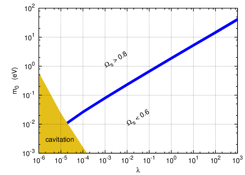
This system of equation is difficult to solve analytically. However we obtain such a relation numerically, thanks to the bisection algorithm implemented in CLASS. Namely, we vary $\lambda$ in the range $[10^{-10},10^{3}]$, $h$ in the range $[0.65,0.75]$, $\Omega_{m}=1-\Omega_{s}$ in the range $[0.2,0.4]$ and obtain the corresponding $m_{0}$ in each case. We show in the left panel of figure 2 the corresponding region in ($\lambda$, $m_{0}$) space (thin blue band). This region is compatible with hydrodynamical constraints only in the range $\lambda>2\times 10^{-5}$ (otherwise the fluid is broken apart by cavitation), corresponding to $m_{0}>0.01$ eV. The fluid is always in local equilibrium in this range of coupling. The scaling between $\lambda$ and $m_{0}$ changes around the value $\lambda\sim 10^{-5}$, but in the physically interesting range $\lambda\gg 10^{-5}$ we find a fitting formula accurate at the percent level:

Note that the validity of the model for a large self-coupling constant is far from obvious, since the expression for bulk viscosity is obtained using perturbation theory and assumes $\lambda<1$. If we impose a theoretical prior $\lambda\leq 1$, the allowed range for the mass reduces to $m_{0}\in[0.01,2]$ eV.

We checked numerically that the above relation between $m_{0}$ and $\lambda$ is not affected by $\epsilon$, as expected from our previous reasoning. Moreover, the current ratio $x^{0}=m_{0}/T_{s}^{0}$ depends on $(\lambda,H_{0},\Omega_{s})$ but not on $\epsilon$. Hence the $\epsilon$ parameter is only important at early time through its impact on the total radiation density.

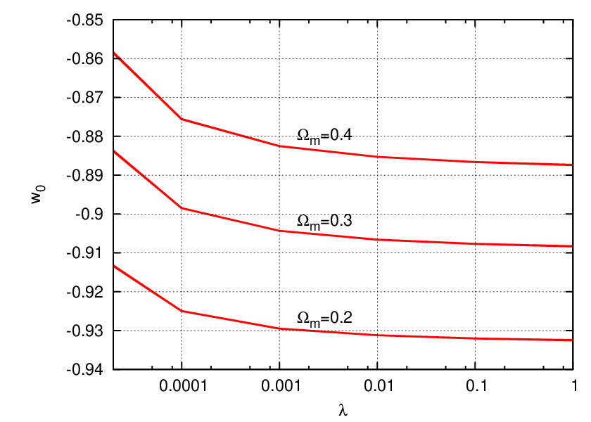
We see from figure 1 that the viscous fluid does not reach the fixed point (or stabilize with a constant energy density) immediately. This suggests that our model predicts a value of the equation-of-state parameter $w=p_{s}/\rho_{s}$ larger than -1 today and slightly varying with time. A priori, the current value $w_{0}$ could depend on $(\lambda,H_{0},\Omega_{s})$ and even slightly on $\epsilon$. A careful numerical investigation illustrated by the right panel of figure 2 shows that $w_{0}$ depends only on $\lambda$ and $\Omega_{s}$ (or $\Omega_{m}$). The same appears to be true for its time-derivative. This seems to imply that the present model is an example of a bulk viscosity-induced dark energy model that does not “cross the phantom divide” Nojiri and Odintsov (2005); Capozziello et al. (2006); Brevik and Gorbunova (2005).

In summary of this subsection, we find that the model under consideration has the same background evolution as a minimal $\Lambda$CDM model extended in the following way:

• •

  It has extra relativistic degrees of freedom at early times, controlled by the parameter $\epsilon$. The equivalent effective neutrino number is

  $$N_{\rm eff}=3.04+2.2\epsilon^{4}~.$$

  (28)

  If scalar particles decouple from the rest of the plasma very late (but before electron-positron annihilation), $\epsilon$ may be in the range $[0.5,0.7]$ and produce a significant increase of $N_{\rm eff}$ ²² 2 Indeed, if the bosons decouple before electron-positron annihilation, their temperature is at most equal to that of neutrinos, $T_{\nu}=(4/11)^{1/3}T_{\gamma}\simeq 0.7T_{\gamma}$. In principle, it would be possible to assume that our bosons decouple from the plasma after electron-positron annihilation, corresponding to $\epsilon$ in the range [0.7,1]. The physics of Big Bang Nucleosynthesis and photon recombination would then be affected in a more non-trivial way than through $N_{\rm eff}$. We do not consider this case for simplicity.. If they decouple early enough such that $\epsilon<0.5$, the increase in $N_{\rm eff}$ is negligible given the accuracy of future CMB and LSS experiments.

• •

  It incorporates slowly decaying dark energy, so our model mimics the so-called wCDM model Chevallier and Polarski (2001); Linder (2003) rather than $\Lambda$CDM. The value of $w$ today is found to be controlled by ($\Omega_{s}$, $\lambda$) or equivalently by ($\Omega_{m}$, $\lambda$), and the following fit is accurate to better than one percent:

  $$w_{0}=-0.9085+0.21(\Omega_{m}-0.3)+3\lambda^{-0.4}10^{-4}~.$$

  (29)

• •

  For a very precise description, one should take into account the fact that the parameter $w$ varies slowly with time during dark energy domination. If we try to capture this small redshift variation with a standard first-order expansion of the type $w(a)=w_{0}+w_{a}(1-a/a_{0})$ Chevallier and Polarski (2001); Linder (2003), we find numerically that the fit

  $$w_{a}=0.129+0.02(\Omega_{m}-0.3)+\lambda^{-0.5}10^{-4},$$

  (30)

  is accurate up to 5%.

It remains to be checked that the equivalence between our model and such an extended wCDM model is valid also at the level of perturbations. The study of linear perturbations is the object of section 4.

Since for $\lambda\gg 10^{-4}$ the scalar fluid undergoes a non-relativistic regime with $\rho_{s}\propto a^{-3}$ prior to the dark energy regime, one could think that it could play alternatively the role of dark matter and dark energy. At the level of the background evolution, this could be achieved by setting $\Omega_{cdm}=0$, $\Omega_{m}=\Omega_{s}+\Omega_{b}=1$, and by increasing $\lambda$ (and hence $m_{0}$) until the scalar density during the non-relativistic regime matches the usual CDM density. We find that this is indeed possible, but for values of $\lambda$ much larger than one. We conclude that our bulk viscosity model cannot explain dark matter and dark energy at the same time, but in principle one could try to extend this model with such a goal.

Our starting point are the standard evolution equations for scalar perturbations in the synchronous gauge (we follow the conventions of Weinberg Weinberg (b)):

where $\rho$ and $p$ are the background values for the density and pressure, $\delta\rho$ and $\delta p$ are the pertubations in density and pressure, $\delta U_{i}=\partial_{i}\delta U+\delta U_{i}^{V}$ are the velocity perturbations (where $\partial_{i}\delta U_{i}^{V}=0$), $\psi$ is a linear combination of metric perturbations, $\pi^{S}$ is the anisotropic stress tensor, $k$ is a wavevector and dots represent derivatives with respect to proper time. Equations 31 and  32 correspond to energy conservation and momentum conservation, respectively. There is one set of energy-momentum conservation equations for each type of matter that does not exchange energy and momentum with other constituents. In the following we present the treatment of linear perturbations for the added scalar matter, but it must be borne in mind that we consider all linear perturbations in our final analysis.

By assumption the scalar fluid in our model only interacts gravitationally with other particles. Thus we can write a set of energy-momentum conservation equations for the scalar perturbations $\delta\rho_{s}$ and $\delta U_{s}$. Since equations 31– 33 do not depend on the particular form of the energy-momentum tensor, we make the replacements $p\rightarrow p_{\rm eff}$ and $\delta p\rightarrow\delta p_{\rm eff}$ to account for bulk viscous effects. We also assume that the anisotropic stress tensor $\pi^{S}$ for our scalar fluid is zero. There is no data to constrain this number and we make this assumption to simplify the equations. The evolution equations of perturbations for our scalar fluid read:

where the subscript “$s$” refer to the scalar fluid and “other” to the other fluids present (photons, neutrinos, baryons, dark matter). We note that all fluid perturbations are necessary to obtain the correct metric perturbations.

In our model, the forms of $\rho_{s}$ and $p_{\rm eff}$ are given in eqs. 16– 18. We note that the energy density is only a function of $x$. So we can express a perturbation in energy density solely as a perturbation in $x$ (or equivalently a change in temperature):

where the function $D(x)=\rho_{s}^{\prime}(x)$ is given by eq. 21. The change in effective pressure is a bit more tricky, since $p_{\rm eff}$ also depends on $D_{\gamma}U^{\gamma}$. We write:

where the function $P_{\rm eff}(x)$ can be obtained from eqs. 16 and 18. To obtain $\delta(D_{\gamma}U^{\gamma})$, we write:

where in the last line we used $\Gamma_{\nu\lambda}^{\nu}(\delta U^{\lambda})=(\Gamma_{0\lambda}^{0}+\Gamma_{i\lambda}^{i})\delta U^{\lambda}=\Gamma_{i0}^{i}\delta U^{0}+\Gamma_{ij}^{i}\delta U^{j}=(3\dot{a}/a)\delta U^{0}$ when spatial curvature is zero. The 4-velocity is $U^{\mu}=(-1,v^{i})$ and thus $\delta U^{0}=0$. Keeping only linear terms in velocity and perturbations and using the perturbed Christoffel symbols in the synchronous gauge Weinberg (b), we obtain:

The perturbation of the effective pressure can thus be expressed in terms of temperature, velocity and metric perturbations:

Using eqs. 37 and 41, we can re-write the evolution equations for the perturbations 34– 36 as:

These are the evolution equations for scalar perturbations for the viscous (scalar) fluid. We integrate them using CLASS and the results are shown in section 4.2. For completness and in order to make our results easily reproducible, we provide in Appendix A a complete list of the equations added to the CLASS perturbation module. Essentially, these are equations 34, 35 and 41 translated into the notations of Ma & Bertschinger Ma and Bertschinger (1995), which are used throughout the CLASS code.

We first study the evolution of a few characteristic scales related to perturbations in the viscous fluids. For a perfect fluid, the qualitative behavior of perturbations is essentially captured by the Jeans wavenumber:

where $c_{i}$ is the sound speed in the fluid. Note that the sound speed is usually defined as the variation of the pressure with respect to the density for constant entropy. Since a viscous fluid contains entropy perturbations, we cannot readily obtain $c_{s}^{2}$ from the ratio $\delta p_{\rm eff}/\delta\rho_{s}$. We should instead bear in mind that the viscosity of the fluid remains negligible in an adiabatic transformation, so we must define the sound speed for the scalar fluid using the equilibrium pressure:

The Jeans wavenumber obtained with $c_{i}=c_{s}$ is shown as a solid blue line in figure 3 (for the same reference model as in the previous section). For comparison, the dashed line is obtained using $c_{i}^{2}=P_{\rm eff}(x)/D(x)$, in order to give an indication of when the viscosity becomes important and which scales it can affect.

Let us now summarize the expected behavior of perturbations in the scalar fluid when their wavenumbers cross the four different regions shown in figure 3 (left). After crossing the Hubble radius $k=aH$, the modes experience gravitational collapse as long as $k<k_{J}$. This stage is very brief: even if the scalar particles become non-relativistic before the dark-energy-like stage (as it is the case in our reference model), the sound speed decreases very slowly below $1/\sqrt{3}$ and the Jeans wavenumber remains of the same order of magnitude as $aH$. When the modes cross the Jeans length ($k>k_{J}$), and as long as viscosity is negligible, acoustic waves start to propagate in the fluid with a velocity $c_{s}$. In Fourier space, $\delta_{s}$ oscillates with a pulsation $kc_{s}$.

At some point, viscosity becomes important, and due to non-adiabatic contributions $|\delta p_{\rm eff}|$ becomes very large with respect to $c_{s}|\delta\rho_{s}|$. In our reference model, this happens around $\tau=3000$ Mpc, since this is the time at which the two characteristic scales plotted in figure 3 become different. The very large value of $|\delta p_{\rm eff}/\delta\rho_{s}|$ implies that the friction term in the equation of propagation of $\delta_{s}$ drives the perturbation to zero, on a time scale shorter than the period of oscillation. This is the regime in which viscosity erases all perturbations in the fluid.

All these expectations can be checked in figure 3 (right). For the reference model, the mode $\delta_{s}(k=10^{-3}\mathrm{Mpc})$ experiences a very short stage of gravitational amplification and is then driven to zero. The mode $\delta_{s}(k=10^{-2}\mathrm{Mpc})$ has three visible stages: amplification, oscillation (for just half-a-period) and damping. The mode $\delta_{s}(k=10^{-1}\mathrm{Mpc})$ is already in the acoustic oscillation phase at the earliest time shown in the figure. Around $\tau=3000$ Mpc, it also experiences a brutal viscosity damping.

The conclusion of this section is that the viscous fluid perturbations never grow significantly during matter domination and are washed out when viscosity becomes important (i.e. prior to dark energy perturbation). From this point of view, our viscous fluid model should be indistinguishable from any other dark energy model with negligible perturbations, like e.g. a scalar field with $c_{s}=1$.

The only time at which the viscous fluid perturbation can play a role is in the radiation domination epoch. During that stage, the fluid dilutes like $\rho_{s}\propto a^{-4}$ and from the background point of view it can be treated as extra massless neutrino species, as explained in section 3.2. This is not obvious at the perturbation level, since decoupled massless neutrinos are collisionless with anisotropic pressure leading to shear viscosity damping. Instead, our fluid is self-coupled and we assume its anisotropic stress to vanish. Hence, during radiation domination and before the time at which viscosity becomes important, we expect $\delta_{s}$ to oscillate with a larger amplitude than $\delta_{\nu}$, even if these two fluid share the same initial conditions and background evolution. This effect could in principle be significant. For instance, it has been proved that the damping of neutrino oscillations caused by shear viscosity is measurable with WMAP data De Bernardis et al. (2008). If detectable, this effect would lead to slightly higher CMB peaks in the viscous model than in a wCDM model with the same $N_{\rm eff}$.

These expectations can be checked by running CLASS for a pair of models: a viscous fluid model and an extended wCDM model with the same values of ($N_{\rm eff}$, $w_{0}$, $w_{a}$) obtained with the fitting formulas 28–30. For such pairs of models and three choices of parameters (same as in section 3.2), we present in figure 4 the CMB temperature and matter power spectra. For the model with $\epsilon=0.1$ ($N_{\rm eff}\simeq 3.04$), the matching is impressive and confirms our expectations. For the other two models with $\epsilon=0.7$ ($N_{\rm eff}\simeq 3.57$), slightly larger CMB peaks can indeed be observed in the viscous model, for the reason explained above. This effect is however small, and we recall that $\epsilon=0.7$ is an extreme assumption: it implies that the scalar particles decouple from the thermal bath late enough so that no entropy creation occured afterwards, except at the time of electron-positron annihilation.

References

- Riess et al. [1998] Adam G. Riess et al. Observational Evidence from Supernovae for an Accelerating Universe and a Cosmological Constant. Astron. J., 116:1009–1038, 1998. doi: 10.1086/300499.
- Perlmutter et al. [1999] S. Perlmutter et al. Measurements of Omega and Lambda from 42 High-Redshift Supernovae. Astrophys. J., 517:565–586, 1999. doi: 10.1086/307221.
- Komatsu et al. [2011] E. Komatsu et al. Seven-Year Wilkinson Microwave Anisotropy Probe (WMAP) Observations: Cosmological Interpretation. Astrophys. J. Suppl., 192:18, 2011. doi: 10.1088/0067-0049/192/2/18.
- Eisenstein et al. [2005] Daniel J. Eisenstein et al. Detection of the Baryon Acoustic Peak in the Large-Scale Correlation Function of SDSS Luminous Red Galaxies. Astrophys. J., 633:560–574, 2005. doi: 10.1086/466512.
- Tegmark et al. [2006] Max Tegmark et al. Cosmological Constraints from the SDSS Luminous Red Galaxies. Phys. Rev., D74:123507, 2006. doi: 10.1103/PhysRevD.74.123507.
- [6] S Amendola, L.and Tsujikawa. Dark energy: Theory and observations. Cambridge, UK: Univ. Pr. (2010) 491 p.
- Frieman et al. [2008] Joshua Frieman, Michael Turner, and Dragan Huterer. Dark Energy and the Accelerating Universe. Ann. Rev. Astron. Astrophys., 46:385–432, 2008. doi: 10.1146/annurev.astro.46.060407.145243.
- Li et al. [2011] Miao Li, Xiao-Dong Li, Shuang Wang, and Yi Wang. Dark Energy. 2011.
- Caldwell and Kamionkowski [2009] Robert R. Caldwell and Marc Kamionkowski. The Physics of Cosmic Acceleration. Ann. Rev. Nucl. Part. Sci., 59:397–429, 2009. doi: 10.1146/annurev-nucl-010709-151330.
- Brax [2009] Philippe Brax. Gif Lectures on Cosmic Acceleration. 2009.
- Caldwell et al. [1998] R. R. Caldwell, Rahul Dave, and Paul J. Steinhardt. Cosmological Imprint of an Energy Component with General Equation-of-State. Phys. Rev. Lett., 80:1582–1585, 1998. doi: 10.1103/PhysRevLett.80.1582.
- Uzan [1999] Jean-Philippe Uzan. Cosmological scaling solutions of non-minimally coupled scalar fields. Phys. Rev., D59:123510, 1999. doi: 10.1103/PhysRevD.59.123510.
- Amendola [2000] Luca Amendola. Coupled quintessence. Phys. Rev., D62:043511, 2000. doi: 10.1103/PhysRevD.62.043511.
- Chiba [1999] Takeshi Chiba. Quintessence, the gravitational constant, and gravity. Phys. Rev., D60:083508, 1999. doi: 10.1103/PhysRevD.60.083508.
- Rasanen [2004] Syksy Rasanen. Dark energy from backreaction. JCAP, 0402:003, 2004. doi: 10.1088/1475-7516/2004/02/003.
- Kolb et al. [2006] Edward W. Kolb, S. Matarrese, and A. Riotto. On cosmic acceleration without dark energy. New J. Phys., 8:322, 2006. doi: 10.1088/1367-2630/8/12/322.
- Buchert [2008] Thomas Buchert. Dark Energy from Structure - A Status Report. Gen. Rel. Grav., 40:467–527, 2008. doi: 10.1007/s10714-007-0554-8.
- Tomita [2000] Kenji Tomita. Distances and lensing in cosmological void models. Astrophys. J., 529:38, 2000. doi: 10.1086/308277.
- Celerier [2000] Marie-Noelle Celerier. Do we really see a cosmological constant in the supernovae data ? Astron. Astrophys., 353:63–71, 2000.
- Padmanabhan and Chitre [1987] T. Padmanabhan and S. M. Chitre. Viscous universes. Phys. Lett., A120:433–436, 1987. doi: 10.1016/0375-9601(87)90104-6.
- Murphy [1973] G. L. Murphy. Big-bang model without singularities. Phys. Rev., D8:4231–4233, 1973. doi: 10.1103/PhysRevD.8.4231.
- Belinskii and Khalatnikov [1975] V.A. Belinskii and I.M. Khalatnikov. Influence of viscosity on the character of cosmological evolution. Zh. Eksp. Teor. Fiz., 69:401, 1975. (Sov. Phys. JETP 42 (1976) 205).
- Fabris et al. [2006] Julio Cesar Fabris, S. V. B. Goncalves, and R. de Sa Ribeiro. Bulk viscosity driving the acceleration of the Universe. Gen. Rel. Grav., 38:495–506, 2006. doi: 10.1007/s10714-006-0236-y.
- Colistete et al. [2007] R. Colistete, J. C. Fabris, J. Tossa, and W. Zimdahl. Bulk Viscous Cosmology. Phys. Rev., D76:103516, 2007. doi: 10.1103/PhysRevD.76.103516.
- Li and Barrow [2009] Baojiu Li and John D. Barrow. Does Bulk Viscosity Create a Viable Unified Dark Matter Model? Phys. Rev., D79:103521, 2009. doi: 10.1103/PhysRevD.79.103521.
- Velten and Schwarz [2011] Hermano Velten and Dominik J. Schwarz. Constraints on dissipative unified dark matter. 2011.
- Kamenshchik et al. [2001] Alexander Yu. Kamenshchik, Ugo Moschella, and Vincent Pasquier. An alternative to quintessence. Phys. Lett., B511:265–268, 2001. doi: 10.1016/S0370-2693(01)00571-8.
- Wilson et al. [2007] James R. Wilson, Grant J. Mathews, and George M. Fuller. Bulk Viscosity, Decaying Dark Matter, and the Cosmic Acceleration. Phys. Rev., D75:043521, 2007. doi: 10.1103/PhysRevD.75.043521.
- Mathews et al. [2008] G. J. Mathews, N. Q. Lan, and C. Kolda. Late Decaying Dark Matter, Bulk Viscosity and the Cosmic Acceleration. Phys. Rev., D78:043525, 2008. doi: 10.1103/PhysRevD.78.043525.
- Jeon [1995] Sangyong Jeon. Hydrodynamic transport coefficients in relativistic scalar field theory. Phys. Rev., D52:3591–3642, 1995. doi: 10.1103/PhysRevD.52.3591.
- Lesgourgues [2011] Julien Lesgourgues. The Cosmic Linear Anisotropy Solving System (CLASS) I: Overview. 2011.
- Blas et al. [2011] Diego Blas, Julien Lesgourgues, and Thomas Tram. The Cosmic Linear Anisotropy Solving System (CLASS) II: Approximation schemes. 2011.
- Weinberg [a] S Weinberg. Gravitation and Cosmology. a. John Wiley and Sons, New York U.S.A. (1972) 657 p.
- [34] J. I. Kapusta and Charles Gale. Finite-temperature field theory: Principles and applications. Cambridge, UK: Univ. Pr. (2006) 428 p.
- Szydlowski and Hrycyna [2007] Marek Szydlowski and Orest Hrycyna. Dissipative or conservative cosmology with dark energy? Annals Phys., 322:2745–2775, 2007. doi: 10.1016/j.aop.2007.06.008.
- Israel and Stewart [1979] W. Israel and J.M. Stewart. Transient relativistic thermodynamics and kinetic theory. Annals Phys., 118:341–372, 1979. doi: 10.1016/0003-4916(79)90130-1.
- Piattella et al. [2011] Oliver F. Piattella, Julio C. Fabris, and Winfried Zimdahl. Bulk viscous cosmology with causal transport theory. JCAP, 1105:029, 2011. doi: 10.1088/1475-7516/2011/05/029.
- Denicol et al. [2008] G.S. Denicol, T. Kodama, T. Koide, and Ph. Mota. Stability and Causality in relativistic dissipative hydrodynamics. J.Phys.G, G35:115102, 2008. doi: 10.1088/0954-3899/35/11/115102.
- Pu et al. [2010] Shi Pu, Tomoi Koide, and Dirk H. Rischke. Does stability of relativistic dissipative fluid dynamics imply causality? Phys.Rev., D81:114039, 2010. doi: 10.1103/PhysRevD.81.114039.
- [40] C. E. Brennen. Cavitation and bubble dynamics. Oxford Univ. Pr. (1995) 294 p.
- Rajagopal and Tripuraneni [2010] Krishna Rajagopal and Nilesh Tripuraneni. Bulk Viscosity and Cavitation in Boost-Invariant Hydrodynamic Expansion. JHEP, 03:018, 2010. doi: 10.1007/JHEP03(2010)018.
- Nojiri and Odintsov [2005] Shin’ichi Nojiri and Sergei D. Odintsov. Inhomogeneous equation of state of the universe: Phantom era, future singularity and crossing the phantom barrier. Phys. Rev., D72:023003, 2005. doi: 10.1103/PhysRevD.72.023003.
- Capozziello et al. [2006] Salvatore Capozziello, V. F. Cardone, E. Elizalde, S. Nojiri, and S. D. Odintsov. Observational constraints on dark energy with generalized equations of state. Phys. Rev., D73:043512, 2006. doi: 10.1103/PhysRevD.73.043512.
- Brevik and Gorbunova [2005] Iver H. Brevik and O. Gorbunova. Dark Energy and Viscous Cosmology. Gen. Rel. Grav., 37:2039–2045, 2005. doi: 10.1007/s10714-005-0178-9.
- Chevallier and Polarski [2001] Michel Chevallier and David Polarski. Accelerating universes with scaling dark matter. Int. J. Mod. Phys., D10:213–224, 2001. doi: 10.1142/S0218271801000822.
- Linder [2003] Eric V. Linder. Exploring the expansion history of the universe. Phys. Rev. Lett., 90:091301, 2003. doi: 10.1103/PhysRevLett.90.091301.
- Weinberg [b] Steven Weinberg. Cosmology. b. Oxford, UK: Oxford Univ. Pr. (2008) 593 p.
- Ma and Bertschinger [1995] Chung-Pei Ma and Edmund Bertschinger. Cosmological perturbation theory in the synchronous and conformal Newtonian gauges. Astrophys.J., 455:7–25, 1995. doi: 10.1086/176550.
- De Bernardis et al. [2008] Francesco De Bernardis, Luca Pagano, Paolo Serra, Alessandro Melchiorri, and Asantha Cooray. Anisotropies in the Cosmic Neutrino Background after WMAP 5-year Data. JCAP, 0806:013, 2008. doi: 10.1088/1475-7516/2008/06/013.
- Izotov and Thuan [2010] Y.I. Izotov and T.X. Thuan. The primordial abundance of 4He: evidence for non-standard big bang nucleosynthesis. Astrophys.J., 710:L67–L71, 2010. doi: 10.1088/2041-8205/710/1/L67. * Temporary entry *.
- Keisler et al. [2011] R. Keisler, C.L. Reichardt, K.A. Aird, B.A. Benson, L.E. Bleem, et al. A Measurement of the Damping Tail of the Cosmic Microwave Background Power Spectrum with the South Pole Telescope. 2011. * Temporary entry *.
- Amanullah et al. [2010] R. Amanullah, C. Lidman, D. Rubin, G. Aldering, P. Astier, et al. Spectra and Light Curves of Six Type Ia Supernovae at 0.511 ¡ z ¡ 1.12 and the Union2 Compilation. Astrophys.J., 716:712–738, 2010. doi: 10.1088/0004-637X/716/1/712.