A precise isospin analysis of decays
Abstract
We present a precise isospin analysis of the decays using new recent experimental measurements on these final states. The decays , originating from transitions, are linked by a rich set of isospin properties. The isospin relations that connect the decay modes are presented and a fit is performed to obtain the isospin amplitudes and phases. We discuss the results of the fit and present a new measurement of the ratio of branching fractions and . We finally discuss the implications of our findings for the measurement of the unitarity matrix parameters and using these decays.
1 Introduction
In this Letter, we use an isospin analysis to establish relations between the different decays. These decays proceed via transitions, which are known to present peculiar isospin properties [1]. The possibility that a large fraction of decays hadronize as was first suggested in Ref. [2] in the context of the discrepancy between the measured semi-leptonic rate and the theoretical prediction. This hypothesis was confirmed by many experimental results where it was found that decays account for about of the and decays [3, 4, 5]. These results provide the input for the isospin analysis and the test of the isospin relations. An additional motivation for an in-depth study of these channels is the possibility, originally discussed in Refs. [6, 7, 8], to measure and using these decays. Indeed they proceed through the same quark current than the gold-plated mode and are not Cabibbo-suppressed to the difference of the modes.
This Letter, which updates and supersedes a previous investigation reported in Ref. [9], presents the complete set of isospin relations for decays. They are compared to the measurements through a fit of the experimental data which determines the isospin amplitudes. There are 22 possible modes for the decays; here the is either a or a , the is either a , , , or , the is the charge conjugate of , and the is either a or a .
These decays have been the object of many experimental investigations during the past years. In particular, the BABAR Collaboration [5] published recently a complete set of measurements of the 22 branching fractions with an excellent accuracy. They used events collected at the resonance, corresponding to an integrated luminosity of . The Belle Collaboration performed a measurement of the branching fractions of the modes [10] and [11] using pairs. All these results are used in our analysis.
With respect to the previous study [9], the statistical and systematic precision on the experimental data is improved by a factor three or larger, thereby improving by the same amount the statistical power of the tests performed. This allows to put on a firm ground the conclusion that we draw from this study.
In addition to the higher statistics, another improvement of the analysis shown in this Letter is the fact that the branching ratios and , needed to compare the neutral to charged meson decays measured at an machine operating at the resonance, are presently known with a good accuracy. This good knowledge of the ratio helps to constrain more strongly the fit performed here.
The aim of this study is:
- 1.
to verify the isospin relations using a new set of precise experimental results;
- 2.
to provide some insight into the decay mechanism from the inspection of the isospin amplitudes;
- 3.
to discuss the implications of our findings for the measurement of and using these decays.
It has to be noted that other authors [12] studied decays in the context of color rearrangement models, and compared their predictions with the experimental measurements.
2 Isospin relations for decays
A full derivation and discussion of the isospin relations for these decays can be found in Ref. [9]. Here only the main results is summarized.
The decays proceed via a current through the diagrams of Fig. 1. Depending on the final state, the external W-emission diagram, the internal W-emission diagram (which is color-suppressed), or both contribute to the transition amplitude. A penguin diagram, shown in Fig. 2 (left plot), can also contribute to the current. It is expected to be suppressed relatively to the tree diagrams of Fig. 1 and does not modify the isospin relations.


The decays and could also proceed through a different diagram, shown in Fig. 2 (right plot), which could introduce a amplitude. However this diagram proceeds through two suppressed weak vertices and and a pair must be extracted from the vacuum, instead of a light quark pair as in the Cabibbo-allowed diagrams. This amplitude is therefore suppressed by at least a factor , where is the expansion parameter of the Wolfenstein parametrization. For these reasons we expect that holds to an excellent precision.
As already mentioned, the isospin properties of the current are well known and follow from the fact that only isoscalar quarks are involved. Therefore this is a weak transition and the final state is an isospin eigenstate.
The isospin properties translate in the following set of relations [9]
| (1) | |||||
| (2) | |||||
| (3) |
where () is the amplitude to produce the system with an isospin quantum number equal to 1 (0). The amplitudes in these formulae are reduced matrix elements, in the terms of the Wigner-Eckart theorem, of the isoscalar Hamiltonian.
A similar set of relations holds for charged B meson decays
| (4) | |||||
| (5) | |||||
| (6) |
where the amplitudes are the same as for the neutral B decays. Identical equations hold for the other set of decays, , and , with different amplitudes in each case. Equivalent relations can be obtained considering the isospin quantum numbers of different subsystems of the final state (, ). The subsystem is chosen here because in this case the transitions of Eqs. (3) and (6), proceeding only through the color-suppressed diagrams of Fig. 1 (left plot), are associated only to the amplitude.
The relations presented above can be cast in the form of a triangle relation between the amplitudes:
| (7) | |||||
| (8) |
which are depicted in Fig. 3. The two triangles for and decays are identical according to the isospin relations, however experimentally it is advantageous to build the triangles separately with the and amplitudes.


We finally notice that Eqs. (1) to (8) are valid not only for the total decay amplitude but also for each helicity amplitude separately as well as for the amplitude as a function of the Dalitz plot coordinates. The amplitudes and phases we extract from the fit are averaged over the Dalitz plot as well as over all the accessible final states (vector polarizations, partial waves, …). This remark is of particular importance since it is now well known that many resonances are present in the decays, such as the , the , the , and the mesons [13].
3 Study of the experimental results
The branching fractions for the charged and neutral meson decay can be written
| (9) | |||||
| (10) |
where and [14] are the lifetimes of the and mesons, and are the masses of the and mesons, and are the invariant masses of the and subsystems, and the integral is computed numerically over the allowed region of the three-body phase space.
The BABAR Collaboration has recently studied the full set of decays and has provided precise measurements for all these modes [5]. We use also the experimental results from the Belle Collaboration [10, 11] which are available for the modes and . These two modes from Belle are combined with the corresponding ones from BABAR assuming fully correlated systematic uncertainties. Table 1 presents the measurements of the final states after having combined the BABAR and Belle results.
The BABAR and Belle data have been collected at the PEP-II and KEKB accelerators from the reaction . To compute the branching fractions, it has been assumed that . However these equalities do not necessarily hold. In order to account for this factor, we rewrite Eqs. (9) and (10) in term of the rescaled amplitudes
| (11) |
The expression for is then multiplied by the additional factor
| (12) |
The experimental data are fitted simultaneously using the method:
| (13) |
where represents the vector of the branching fraction measurements, represents the vector of the branching fraction predictions, and the superscript denotes the transposed vector. The predictions depend on 13 parameters which are and, for each set of decays, , , and . The matrix is the covariance matrix between the 22 branching fraction measurements, which allows to take properly into account the systematic uncertainties that are common and correlated between each mode. The correlated systematic uncertainties consist of uncertainties originating from the signal shape, the reconstruction and the identification of particles (charged tracks, soft pions from decays, , , single photon, and identification), the branching fractions of the secondary decays ( and ), and the accounting of the number of pairs produced in the experiment (see Table III of Ref. [5]). We separate each contribution of these systematic effects in order to break down the problem into quantities which are completely independent or completely correlated. We sum these separate covariance matrices together to obtain the total covariance matrix, where the partial correlation structures emerge. The last term in Eq. (13) constrains to the world average value [14].
The results of the minimization of this are reported in Tables 1 and 2. The overall agreement between the measured and predicted branching fractions is fair as can be judged from Table 1, Figs. 4 and 5, and from the value for 10 degrees of freedom () with a probability of 4.1%. We observe that the main source of the disagreement concerns the modes containing one or two mesons, with a measured branching fraction systematically above the predicted value. This could point to a systematic shift that was not properly taken into account in the experimental analysis. For some decays which are not distinguishable experimentally, only the sum of the branching fraction with the charge conjugate final state has been measured. We present in Table 3 the fitted values for the individual branching fractions.
The fit has also been conducted without the constraint on . We obtain a value
| (14) |
which is in good agreement, while less precise, with the world average.
An alternative way of displaying the experimental results and the fit results is given by the isospin triangles introduced in the above. For ease of comparison, we normalize the triangles to the size of the basis ( and ): therefore the lower side extends in each case from (0,0) to (1,0) and the shapes of the triangles can be directly compared. Given that we have only a measurement of the sides, there is a fourfold ambiguity on the vertex of the triangle. We choose consistently the same solution for its orientation. The seven measured triangles defined in this way are shown in Fig. 6 together with the fit result. We notice that in all the cases the shape of the triangles presents large angles.
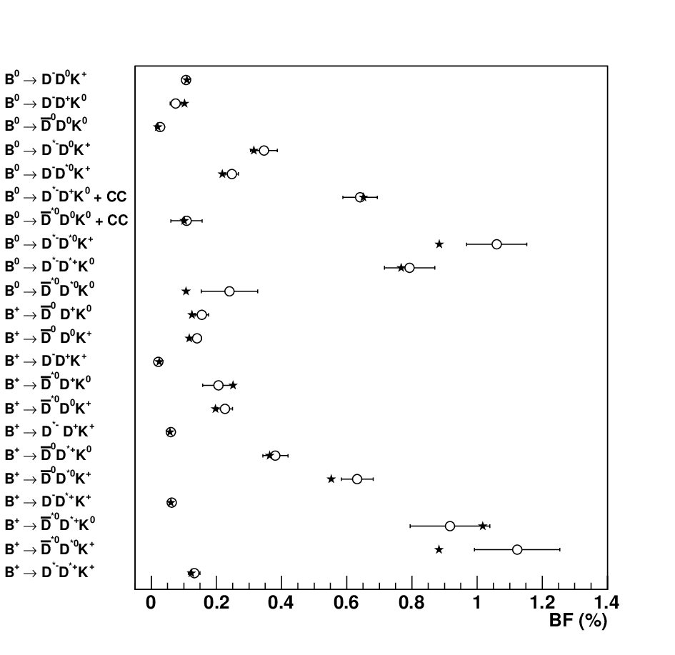
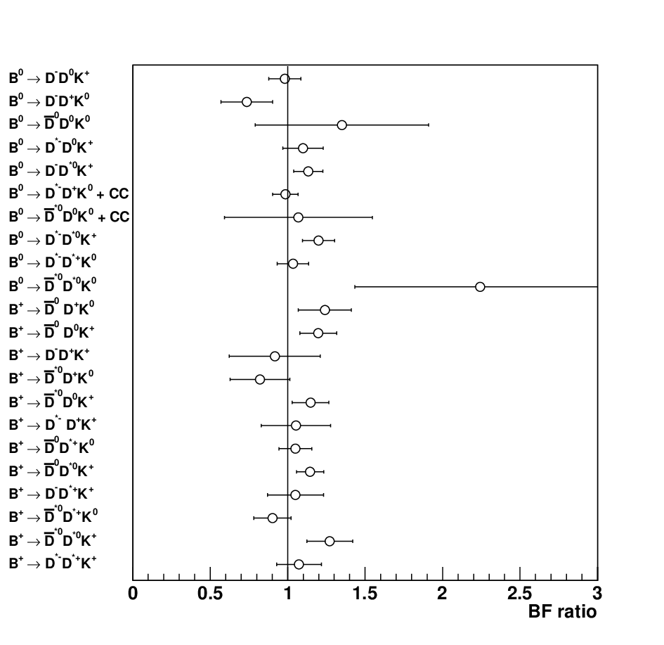
| decay mode | exp. | fit |
| decays through external -emission amplitudes | ||
| 10.9 | ||
| 31.5 | ||
| 21.8 | ||
| 88.4 | ||
| decays through external+internal -emission amplitudes | ||
| 65.1 | ||
| 76.7 | ||
| decays through internal -emission amplitudes | ||
| 10.1 | ||
| decays through external -emission amplitudes | ||
| 25.1 | ||
| 101.7 | ||
| decays through external+internal -emission amplitudes | ||
| 11.7 | ||
| 19.7 | ||
| 88.3 | ||
| decays through internal -emission amplitudes | ||
| 5.7 | ||
| Parameter | Value |
|---|---|
| 18.9/10 | |
| Prob | 4.1 % |
| decay mode | fit |
|---|---|
| 17.1 | |
| 48.0 | |
| 4.9 | |
| 5.2 |

4 Discussion
4.1 Dynamical features of the amplitudes
The amplitudes and phases extracted from the data present some distinctive features. First, within each set, the amplitude related to the color-suppressed decays is much smaller, as expected. The ratios are presented in Table 4. These ratios are very close to the naïve expectation of a suppression factor , where is the number of colors.
Second, the central values for the relative phases are in all cases large and close to . From this we can conclude that there is a firm indication for large strong phases in these amplitudes. This suggests the presence of non-negligible Final State Interaction for these decays. This is both an important indication per se and has also consequences for the violation studies that will be discussed in the next section.
| ratio | value |
|---|---|
4.2 Implications for the measurement of and
All the final states are in principle good candidates for the measurement of the angle of the unitarity matrix [6, 7, 8]. The advantages of these modes, for example with respect to , are that they are Cabibbo-favored and present a small penguin contribution. Since both and can decay to , we expect a time-dependent violating asymmetry. A study of the time-dependent Dalitz plot allows to access the phase related to the and mixing. We notice that for , the measured value of the branching fraction () and the value predicted by our fit () are almost a factor two lower that what was anticipated in Ref. [8], thereby unfortunately also reducing the comparative advantage of this mode with respect to .
The BABAR experiment did a study of the final state in this context and was able to constrain to be positive at the 94% confidence level (under some theoretical and resonant substructure assumptions, and using pairs) [15]. The Belle experiment did a similar analysis on the same final state with pairs and did a measurement of the violation parameters, although the study did not allow to conclude on the sign of [10].
Unfortunately, up to now, no other modes have been studied in the context of violation. From the BABAR data () [5], we see that the final state is observed with a significance of , where is the standard deviation, which shows that a -violation analysis would be possible.
For , a value of is reported (with a significance). In this case too, the estimated value of Ref. [7] () is a factor 12 above the measurement. However, we stress that this channel is a good candidate for -violation studies because of the nature of the final state with three pseudoscalar particles. This will facilitate the angular analysis to determine the helicity amplitudes.
Finally we notice that the and decay modes lead to final states accessible to both and . They can therefore be analyzed in the same way as described in Ref. [16]. The strong phases play an important role for this analysis as the time-dependent -asymmetry amplitudes are proportional to , where is the strong phase difference between and . The possibly large values of the strong phases noticed in the above need to be taken into account for any estimate of the sensitivities of this analysis.
5 Conclusion
We have presented an isospin analysis of the decays, based on recent and precise measurements of these final states. A fit was performed using the isospin relations between the different final states. We find a good agreement between the experimental values and the fitted values. The isospin amplitudes exhibit several peculiar features like the presence of color-suppression and large relative phases. We find a value of equal to , in agreement with other determinations of this quantity. We have discussed the features of our result and showed the implications for -violation measurements using these decays.
6 Acknowledgments
The authors would like to warmly thank Sébastien Descotes-Genon for careful reading of this Letter and useful discussions.
References
- [1] H. J. Lipkin and A. I. Sanda, Phys. Lett. B 201, 541 (1988).
- [2] G. Buchalla, I. Dunietz, and H. Yamamoto, Phys. Lett. B 364, 185 (1995).
- [3] CLEO Collaboration, CLEO CONF 97-26, EPS97 337 (1997); T. E. Coan et al. (CLEO Collaboration), Phys. Rev. Lett. 80, 1150 (1998); R. Barate et al. (ALEPH Collaboration), Eur. Phys. Jour. C 4, 387 (1998).
- [4] B. Aubert et al. (BABAR Collaboration), Phys. Rev. D 68, 092001 (2003).
- [5] P. del Amo Sanchez et al. (BABAR Collaboration), Phys. Rev. D 83, 032004 (2011).
- [6] J. Charles, A. Le Yaouanc, L. Oliver, O. Pene, and J. C. Raynal, Phys. Lett. B 425, 375 (1998) [Erratum-ibid. B 433, 441 (1998)].
- [7] P. Colangelo, F. De Fazio, G. Nardulli, N. Paver, and Riazuddin, Phys. Rev. D 60, 033002 (1999).
- [8] T. E. Browder, A. Datta, P. J. O’Donnell and S. Pakvasa, Phys. Rev. D 61, 054009 (2000).
- [9] M. Zito, Phys. Lett. B 586, 314 (2004).
- [10] J. Dalseno et al. (Belle Collaboration), Phys. Rev. D 76, 072004 (2007).
- [11] J. Brodzicka et al. (Belle Collaboration), Phys. Rev. Lett. 100, 092001 (2008).
- [12] D. Eriksson, G. Ingelman, and J. Rathsman, Phys. Rev. D 79, 014011 (2009).
- [13] J. Brodzicka et al. (Belle Collaboration), Phys. Rev. Lett. 100, 092001 (2008); B. Aubert et al. (BABAR Collaboration), Phys. Rev. D 77, 011102 (2008); T. Aushev, N. Zwahlen et al. (Belle Collaboration), Phys. Rev. D 81, 031103 (2010).
- [14] K. Nakamura et al. (Particle Data Group), J. Phys. G 37, 075021 (2010).
- [15] B. Aubert et al. (BABAR Collaboration), Phys. Rev. D 74, 091101 (2006).
- [16] R. Aleksan et al., Nucl. Phys. B 361, 141 (1991).