跳到论文正文
W Papers独立论文阅读器 arXiv:1107.1404 论文正文 计算阅读时间 · 0%
引用这篇论文根据当前论文元数据生成,正式投稿前建议核对。


License: arXiv.org perpetual non-exclusive license
arXiv:1107.1404v3 [math.ST] 17 Dec 2012

Multiscale Methods for Shape Constraints in Deconvolution: Confidence Statements for Qualitative Features

Johannes Schmidt-Hieber    Axel Munk    Lutz Dümbgen
Abstract

We derive multiscale statistics for deconvolution in order to detect qualitative features of the unknown density. An important example covered within this framework is to test for local monotonicity on all scales simultaneously. We investigate the moderately ill-posed setting, where the Fourier transform of the error density in the deconvolution model is of polynomial decay. For multiscale testing, we consider a calibration, motivated by the modulus of continuity of Brownian motion. We investigate the performance of our results from both the theoretical and simulation based point of view. A major consequence of our work is that the detection of qualitative features of a density in a deconvolution problem is a doable task although the minimax rates for pointwise estimation are very slow.

keywords
[class=AMS] Primary 62G10 ; secondary 62G15 , 62G20
keywords
Brownian motion , convexity , pseudo-differential operators , ill-posed problems , mode detection , monotonicity , multiscale statistics , shape constraints

and

Department of Mathematics
Vrije Universiteit Amsterdam
De Boelelaan 1081a,
1081 HV Amsterdam
Netherlands
??

Institut für Mathematische Stochastik
Universität Göttingen
Goldschmidtstr. 7
D-37077 Göttingen
and
Max-Planck Institute
for Biophysical Chemistry
Am Fassberg 11
D-37077 Göttingen
Germany
??

Institut für mathematische Stochastik
und Versicherungslehre
Universität Bern
Alpeneggstrasse 22
CH-3012 Bern
Switzerland
??

1 Introduction

We observe Y=(Y1,…,Yn)Y=\left(Y_{1},\ldots,Y_{n}\right) according to the deconvolution model

Yi=Xi+ϵi,i=1,…,n,\displaystyle Y_{i}=X_{i}+\epsilon_{i},\quad i=1,\ldots,n, (1)

where Xi,ϵi,i=1,…,nX_{i},\epsilon_{i},\ i=1,\ldots,n are assumed to be real valued and independent, Xi∼i.i.d.X,ϵi∼i.i.d.ϵX_{i}\stackrel{{\scriptstyle i.i.d.}}{{\sim}}X,\epsilon_{i}\stackrel{{\scriptstyle i.i.d.}}{{\sim}}\epsilon and Y1,X,ϵY_{1},X,\epsilon have densities g,fg,f and fϵf_{\epsilon}, respectively. Our goal is to develop multiscale test statistics for certain structural properties of ff, where the density fϵf_{\epsilon} of the blurring distribution is assumed to be known.

Although estimation in deconvolution models has attracted a lot of attention during the last decades (cf. Fan [17], Diggle and Hall [12], Pensky and Vidakovic [41], Johnstone et al. [29], Butucea and Tsybakov [7] as well as Meister [38] for some selective references), inference about ff and its qualitative features is rather less well studied. In fact, adaptive confidence bands would be desirable but turn out to be very ambitious. First, they suffer from the bad convergence rates induced by the ill-posedness of the problem (cf. Bissantz et al. [5]), making confidence bands less attractive for applications. Second, one would need to circumvent the classical problems of honest adaptation over Hölder scales. To overcome these difficulties the aim of the paper is to derive simultaneous confidence statements for qualitative features of f.f.

Structural properties or shape constraints will be conveniently expressed as (pseudo)-differential inequalities of the density ff, assuming for the moment that ff is sufficiently smooth. Important examples are f′≷0f^{\prime}\gtrless 0 to check local monotonicity properties as well as f′′≷0f^{\prime\prime}\gtrless 0 for local convexity or concavity. To give another example, suppose that we are interested in local monotonicity properties of the density f~\tilde{f} of exp⁡(a​X)\exp(aX) for given a>0a>0. Since f~​(s)=(a​s)−1​f​(a−1​log⁡(s))\tilde{f}(s)=(as)^{-1}f(a^{-1}\log(s)), one can easily verify that local monotonicity properties of f~\tilde{f} may be expressed in terms of the inequalities f′−a​f≶0f^{\prime}-af\lessgtr 0.

This paper deals with the moderately ill-posed case, meaning that the Fourier transform of the blurring density fϵf_{\epsilon} decays at polynomial rate. In fact, we work under the well-known assumption of Fan [17] (cf. Assumption 2), which essentially assures that the inversion operator, mapping g↦fg\mapsto f, is pseudo-differential. This combines nicely with the assumption on the class of shape constraints. Our framework includes many important error distributions such as Exponential, χ2\chi^{2}, Laplace and Gamma distributed random variables. The special case ϵ=0\epsilon=0 (i.e. no deconvolution or direct problem) can be treated as well, of course.

1.1 Example: Detecting trends in deconvolution

To illustrate the key ideas, suppose that we are interested in detection of regions of increase and decrease of the true density in Laplace deconvolution, that is, the error density is given by fϵ=(2θ)−1exp(−|⋅|/θ)f_{\epsilon}=(2\theta)^{-1}\exp(-|\cdot|/\theta). Let ϕ\phi be a sufficiently smooth, non-negative kernel function (i.e. ∫ϕ⁡(u)​𝑑u=1\int\phi(u)du=1), supported on [0,1][0,1]. Then, since f=g−θ2​g′′f=g-\theta^{2}g^{\prime\prime} in this case, it follows by partial integration that

Tt,h:=1h​n​∑k=1n(θ2h2​ϕ(3)​(Yk−th)−ϕ′​(Yk−th)).\displaystyle T_{t,h}:=\frac{1}{h\sqrt{n}}\sum_{k=1}^{n}\left(\frac{\theta^{2}}{h^{2}}\phi^{(3)}\left(\frac{Y_{k}-t}{h}\right)-\phi^{\prime}\left(\frac{Y_{k}-t}{h}\right)\right). (2)

has expectation 𝔼​Tt,h=n​∫tt+hϕ⁡(s−th)​f′​(s)​𝑑s\mathbb{E}T_{t,h}=\sqrt{n}\int_{t}^{t+h}\phi(\tfrac{s-t}{h}\big)f^{\prime}(s)ds. The construction of the multiscale test relies on the following analytic observation. Suppose that for a given pair (t,h)(t,h) there is a number dt,hd_{t,h} such that

|Tt,h−𝔼​Tt,h|≤dt,h.\displaystyle|T_{t,h}-\mathbb{E}T_{t,h}|\leq d_{t,h}. (3)

If in addition Tt,h>dt,hT_{t,h}>d_{t,h}, then necessarily

𝔼​Tt,h=n​∫tt+hϕ⁡(s−th)​f′​(s)​𝑑s>0\displaystyle\mathbb{E}T_{t,h}=\sqrt{n}\int_{t}^{t+h}\phi\big(\tfrac{s-t}{h}\big)f^{\prime}(s)ds>0 (4)

and by the non-negativity of ϕ\phi, f⁡(s1)<f⁡(s2)f(s_{1})<f(s_{2}) for some points s1<s2s_{1}<s_{2} in [t,t+h][t,t+h]. On the contrary, Tt,h<−dt,hT_{t,h}<-d_{t,h} implies that there is a decrease on [t,t+h][t,t+h]. For a sequence Nn=o⁡(n/log3⁡n)N_{n}=o(n/\log^{3}n) tending to infinity faster than log3⁡n\log^{3}n and un=1/log⁡log⁡nu_{n}=1/\log\log n, define

Bn:={(kNn,lNn)|k=0,1,…,l=1,2,…,[Nnun],k+l≤Nn}.\displaystyle B_{n}:=\Big\{\Big(\frac{k}{N_{n}},\frac{l}{N_{n}}\Big)\ \big|\ k=0,1,\ldots,\ l=1,2,\ldots,[N_{n}u_{n}],\ k+l\leq N_{n}\Big\}.

Given α∈(0,1)\alpha\in(0,1), we will be able to compute bounds dt,hd_{t,h} such that for all (t,h)∈Bn(t,h)\in B_{n}, inequality (3) holds simultaneously with asymptotic probability 1−α1-\alpha. Taking into account that (3) implies (4), this allows to identify regions of increase and decrease for prescribed probability.

Refer to caption
Fig 1: Simulation for sample size n=2000n=2000 and 90%90\%-quantile. Upper display: True density ff (dashed) and convoluted density gg (solid). Middle display: Kernel density estimates for ff based on the bandwidths h=0.22h=0.22 (’   ’), h=0.31h=0.31 (’   ’), and h=0.40h=0.40 (’  ’). Lower display: Confidence statements. Thick horizontal lines are intervals with monotone increase/decrease (above/below the thin line).

Figure 1 shows a simulation result for n=2000,Nn=⌊n3/5⌋,θ=0.075n=2000,N_{n}=\lfloor n^{3/5}\rfloor,\theta=0.075 and confidence level 90%90\%. The upper panel of Figure 1 displays the true density of ff as well as the convoluted density gg. Notice that we only have observations with density gg. In fact, by visual inspection of gg it becomes apparent how difficult it is to find segments on which ff is monotone increasing/decreasing.

The lower panel of Figure 1 displays intervals for which we can conclude that there is a monotone increase/decrease. Let us give precise instructions on how to read this plot: Pick any of the thick horizontal lines. Then, with overall probability 90%90\%, somewhere in this interval there is a monotone increase or decrease of ff, depending on whether it is drawn above or below the thin line, respectively. In particular, the fact that intervals with monotone increase and decrease overlap does not yield a contradiction, since the statement is that the monotonicity holds only on a non-empty subset of the corresponding interval. (The way the intervals are piled up in the plot, besides the fact that they are above or below the thin line, is arbitrary and does not contain information.) Recall that we have uniformity in the sense that with confidence 90%90\% all these statements are true simultaneously (cf. also Dümbgen and Walther [14]).

To illustrate our approach consider the middle panel in Figure 1. Here, we have displayed three reconstructions using t↦Tt,h/(h​n)t\mapsto T_{t,h}/(h\sqrt{n}) as kernel density estimator with the same unimodal kernel as for the test statistic and three different bandwidths h∈{0.22,0.31,0.40}h\in\{0.22,0.31,0.40\}. Not surprisingly (cf. Delaigle and Gijbels [11]), the reconstructions yield very different answers what the shape of ff could be. For instance, focus on the left hand side of the graph. For h=0.22h=0.22 and h=0.31h=0.31, the density estimators have a mode at around 0.060.06, which is completely smoothed out under the larger bandwidth h=0.4h=0.4. As a practitioner, not knowing the truth, we might want to screen for modes by browsing through the plots for varying bandwidths and ask ourselves whether there is another mode or not. With the confidence statement in the lower display, we see that the true density ff has to have a monotone decrease on [0.02,0.22][0.02,0.22] with confidence 90%90\% (this is exactly the meaning of the leftmost horizontal line). This rules out the reconstruction without a mode at 0.060.06, since it is monotone increasing on the whole interval [0,0.25][0,0.25] and thus does not reflect the right shape behavior. The kernel density estimator corresponding to the smallest bandwidth h=0.22h=0.22 (although it is the best estimator in a pointwise sense) suggests that there could be another mode at around 0.580.58. However, since the confidence intervals do not support such a hypothesis, this could be merely an artefact. Combining the confidence statements in Figure 1, we conclude that with 90%90\% confidence the true density has a local minimum and a local maximum on [0,1][0,1]. Repetition of the simulation shows that often two, three or four segments of increases and decreases are detected, and at most one mode on [0,1][0,1] is found (in 69%69\% of the cases). Therefore, sample size n=2000n=2000 is not large enough to detect systematically the correct number of minima and maxima (22 and 33). Numerical simulations for larger sample size and more details are given in Section 6.

The derived confidence statements should be viewed as an additional tool for analyzing data, in particular for substantiating vague conclusions or visual impressions from point estimators.

1.2 Pseudo-differential operators and multiscale analysis

As mentioned at the beginning of the introduction, we interpret shape constraints as pseudo-differential inequalities. Let ℱ(f)=∫ℝexp(−ix⋅)f(x)dx\mathcal{F}(f)=\int_{\mathbb{R}}\exp\left(-ix\cdot\right)f(x)dx always denote the Fourier transform of f∈L1​(ℝ)f\in L^{1}\left(\mathbb{R}\right) or f∈L2​(ℝ)f\in L^{2}\left(\mathbb{R}\right) (depending on the context). Consider a general class of differential operators op⁡(p)\operatorname{op}(p) with symbol pp which can be written for nice ff as

(op⁡(p)​f)​(x)=12​π​∫ei​x​ξ​p​(x,ξ)​ℱ​(f)​(ξ)​𝑑ξ.\displaystyle(\operatorname{op}(p)f)(x)=\frac{1}{2\pi}\int e^{ix\xi}p(x,\xi)\mathcal{F}(f)(\xi)d\xi. (5)

This class will be an enlargement of (elliptic) pseudo-differential operators by fractional differentiation. Given data from model (1) the goal is then to identify intervals at a controlled error level on which Re⁡(op⁡(p)​f)≰0\operatorname{Re}(\operatorname{op}(p)f)\not\leq 0 or Re⁡(op⁡(p)​f)≱0\operatorname{Re}(\operatorname{op}(p)f)\not\geq 0. Here Re\operatorname{Re} denotes the projection on the real part. In Subsection 1.1 we studied implicitly already the case of op⁡(p)\operatorname{op}(p) being the differentiation operator D​f=f′Df=f^{\prime} (monotonicity). If applied to op⁡(p)=D2\operatorname{op}(p)=D^{2} (i.e. p⁡(x,ξ)=−ξ2p(x,\xi)=-\xi^{2}), our method yields bounds for the number and confidence regions for the location of inflection points of ff. We also discuss an example related to Wicksell’s problem with shape constraint described by fractional differentiation.

The statistic introduced in this paper investigates shape constraints of the unknown density ff on all scales simultaneously. Generalizing (4), we need to derive simultaneous confidence intervals for ⟨ϕ∘St,h,Re⁡(op⁡(p)​f)⟩\langle\phi\circ S_{t,h},\operatorname{Re}(\operatorname{op}(p)f)\rangle with the scale-and-location shift St,h=(⋅−t)/hS_{t,h}=(\cdot-t)/h and the inner product ⟨h1,h2⟩:=∫ℝh1​(x)​h2¯​(x)​𝑑x\langle h_{1},h_{2}\rangle:=\int_{\mathbb{R}}h_{1}(x)\overline{h_{2}}(x)\,dx in L2L^{2}. If op⁡(p)⋆\operatorname{op}(p)^{\star} is the adjoint of op⁡(p)\operatorname{op}(p) (in a certain space) with respect to ⟨⋅,⋅⟩\langle\cdot,\cdot\rangle, then

n​⟨ϕ∘St,h,Re⁡op⁡(p)​f⟩\displaystyle\sqrt{n}\ \big\langle\phi\circ S_{t,h},\operatorname{Re}\operatorname{op}(p)f\big\rangle =n​Re​∫(op⁡(p)⋆​(ϕ∘St,h))​(x)​f​(x)​𝑑x\displaystyle=\sqrt{n}\ \operatorname{Re}\int\big(\operatorname{op}(p)^{\star}(\phi\circ S_{t,h})\big)(x)f(x)dx
=n2​π​Re​∫ℱ⁡(op⁡(p)⋆​(ϕ∘St,h))​(s)​ℱ​(f)​(s)¯​𝑑s\displaystyle=\frac{\sqrt{n}}{2\pi}\ \operatorname{Re}\int\mathcal{F}\big(\operatorname{op}(p)^{\star}(\phi\circ S_{t,h})\big)(s)\overline{\mathcal{F}(f)(s)}ds (6)

and the r.h.s. can be estimated unbiasedly by the test statistic

Tt,h:=n−1/2∑k=1nRevt,h(Yk)T_{t,h}:=n^{-1/2}\sum_{k=1}^{n}\operatorname{Re}\ v_{t,h}(Y_{k})

with

vt,h​(u):=12​π​∫ℱ⁡(op⁡(p)⋆​(ϕ∘St,h))​(s)​ei​s​uℱ​(fϵ)​(−s)​𝑑s.\displaystyle v_{t,h}(u):=\frac{1}{2\pi}\int\mathcal{F}\big(\operatorname{op}(p)^{\star}(\phi\circ S_{t,h})\big)(s)\frac{e^{isu}}{\mathcal{F}(f_{\epsilon})(-s)}ds.

This gives rise to a multiscale statistic

Tn=sup(t,h)wh​(|Tt,h−𝔼​Tt,h|Std⁡(Tt,h)^−w~h),\displaystyle T_{n}=\sup_{(t,h)}w_{h}\left(\frac{\big|T_{t,h}-\mathbb{E}\,T_{t,h}\big|}{\widehat{\operatorname{Std}(T_{t,h})}}-\widetilde{w}_{h}\right),

where whw_{h} and w~h\widetilde{w}_{h} are chosen in order to calibrate the different scales with equal weight, while Std⁡(Tt,h)^\widehat{\operatorname{Std}(T_{t,h})} is an estimator of the standard deviation of Tt,hT_{t,h}.

The key result in this paper is the approximation of TnT_{n} by a distribution-free statistic from which critical values can be inferred. Given the critical values, we can in a second step compute bounds dt,hd_{t,h} such that a statement of type (3) holds. Following the same ideas as in Subsection 1.1, this is enough to identify intervals on which Re⁡(op⁡(p)​f)≰0\operatorname{Re}(\operatorname{op}(p)f)\not\leq 0 or Re⁡(op⁡(p)​f)≱0\operatorname{Re}(\operatorname{op}(p)f)\not\geq 0. In fact the multiscale method implies confidence statements which are stronger than the ones described up to now. These objects can be related to superpositions of confidence bands. For more precise statements see Section 4.

1.3 Comparison with related work and applications

Hypothesis testing for deconvolution and related inverse problems is a relatively new area. Current methods cover testing of parametric assumptions (cf. [4, 34, 6]) and, more recently, testing for certain smoothness classes such as Sobolev balls in a Gaussian sequence model (Laurent et al. [35, 34] and Ingster et al. [28]). All these papers focus on regression deconvolution models. Exceptions for density deconvolution are Holzmann et al. [25], Balabdaoui et al. [3], and Meister [39] who developed tests for various global hypotheses, such as global monotonicity. The latter test has been derived for one fixed interval and allows to check whether a density is monotone on that interval at a preassigned level of significance.

Our work can also be viewed as an extension of Chaudhuri and Marron [8] as well as Dümbgen and Walther [14] who treated the case op⁡(p)=Dm\operatorname{op}(p)=D^{m} (with m=1m=1 in [14]) in the direct case, i.e. when ϵ=0\epsilon=0. However, the approach in [8] does not allow for sequences of bandwidths tending to zero and yields limit distributions depending on unknown quantities again. The methods in [14] require a deterministic coupling result. The latter allows to consider the multiscale approximation for f=𝕀[0,1]f=\mathbb{I}_{[0,1]} only, but it cannot be transferred to the deconvolution setting.

One of the main advantages of multiscale methods, making it attractive for applications, is that essentially no smoothing parameter is required. The main choice will be the quantile of the multiscale statistic, which has a clear probabilistic interpretation. Furthermore, our multiscale statistic allows to construct estimators for the number of modes and inflection points which have a number of nice properties: First, modes and inflection points are detected with the minimax rate of convergence (up to a log-factor). Second, the probability that the true number is overestimated can be made small, since it is completely controlled by the quantile of the multiscale statistic. To state it differently, it is highly unlikely that artefacts are detected, which is a desirable property in many applications. It is worth noting that neither assumptions are made on the number of modes nor additional model selection penalties are necessary.

For practical applications, we may use these models if for instance the error variable ϵ\epsilon is an independent waiting time. For example let XiX_{i} be the (unknown) time of infection of the ii-th patient, ϵi\epsilon_{i} the corresponding incubation time, and YiY_{i} is the time when diagnosis is made. Then, it is convenient to assume ϵ∼Γ⁡(r,θ)\epsilon\sim\Gamma\left(r,\theta\right) (see for instance [10], Section 3.5). By the techniques developed in this paper one will be able to identify for example time intervals where the number of infections increased and decreased for a specified confidence level. Another application is single photon emission computed tomography (SPECT), where the detected scattered photons are blurred by Laplace distributed random variables (cf. Floyd et al. [18], Kacperski et al. [30]).

The paper is organized as follows. In Section 2 we show how distribution-free approximations of multiscale statistics can be derived for general empirical processes under relatively weak conditions. For the precise statement see Theorem 1. These results are transferred to shape constraints and deconvolution models in Section 3. In Section 4 we discuss the statistical consequences and show how confidence statements can be derived. Theoretical questions related to the performance of the multiscale method and numerical aspects are discussed in Sections 5 and 6. Proofs and further technicalities are shifted to the appendix.

Notation: We write 𝒯\mathcal{T} for the set [0,1]×(0,1][0,1]\times(0,1]. The expression ⌊x⌋\lfloor x\rfloor means the largest integer not exceeding xx. The support of a function ϕ\phi is supp⁡ϕ\operatorname{supp}\phi, ∥⋅∥p\|\cdot\|_{p} denotes the norm in Lp:=Lp​(ℝ)L^{p}:=L^{p}(\mathbb{R}), and TV⁡(⋅)\operatorname{TV}(\cdot) stands for the total variation of functions on ℝ\mathbb{R}. As customary in the theory of Sobolev spaces, put ⟨s⟩:=(1+|s|2)1/2\langle s\rangle:=(1+|s|^{2})^{1/2}. One should not confuse this with ⟨⋅,⋅⟩\langle\cdot,\cdot\rangle, the L2L^{2}-inner product. If it is clear from the context, we write xk​ϕx^{k}\phi and ⟨x⟩k​ϕ\langle x\rangle^{k}\phi for the functions x↦xk​ϕ​(x)x\mapsto x^{k}\phi(x) and x↦⟨x⟩k​ϕ​(x)x\mapsto\langle x\rangle^{k}\phi(x), respectively. The (L2L^{2}-)Sobolev space HrH^{r} is defined as the class of functions with norm

‖ϕ‖Hr:=(∫⟨s⟩2​r​|ℱ⁡(ϕ)​(s)|2​𝑑s)1/2<∞.\displaystyle\|\phi\|_{H^{r}}:=\Big(\int\langle s\rangle^{2r}|\mathcal{F}(\phi)(s)|^{2}ds\Big)^{1/2}<\infty.

For any qq and ℓ∈ℕ\ell\in\mathbb{N} (ℕ\mathbb{N} is always the set of non-negative integers) define HℓqH^{q}_{\ell} as the Sobolev type space

Hℓq:={ψ|xkψ∈Hq,fork=0,1,…,ℓ}\displaystyle H^{q}_{\ell}:=\big\{\psi\ |\ x^{k}\psi\in H^{q},\ \text{for}\ k=0,1,\ldots,\ell\ \big\}

with norm ‖ψ‖Hℓq:=∑k=0ℓ‖xk​ψ‖Hq\|\psi\|_{H^{q}_{\ell}}:=\sum_{k=0}^{\ell}\|x^{k}\psi\|_{H^{q}}.

2 A general multiscale test statistic

In this section, we shall give a fairly general convergence result which is of interest on its own. The presented result does not use the deconvolution structure of model (1). It only requires that we have observations Yi=G−1(Ui),i=1,…,nY_{i}=G^{-1}(U_{i}),\ i=1,\ldots,n with UiU_{i} i.i.d. uniform on [0,1][0,1] and GG an unknown distribution function with Lebesgue density gg in the class

𝒢:=𝒢c,C,q:={G|\displaystyle\mathcal{G}:=\mathcal{G}_{c,C,q}:=\big\{G\ \big| G​is a distribution function with density​g,\displaystyle\ G\ \text{is a distribution function with density}\ g,
c≤g|[0,1],∥g∥∞≤c−1,andg∈𝒥(C,q)}\displaystyle\ \ c\leq g\big|_{[0,1]},\ \|g\|_{\infty}\leq c^{-1},\ \text{and}\ g\in\mathcal{J}(C,q)\ \big\} (7)

for fixed c,C≥0c,C\geq 0, 0≤q<1/20\leq q<1/2, and the Lipschitz type constraint

𝒥\displaystyle\mathcal{J} :=𝒥⁡(C,q)\displaystyle:=\mathcal{J}(C,q)
:={h||h⁡(x)−h⁡(y)|≤C(1+|x|+|y|)q|x−y|,for allx,y∈ℝ}.\displaystyle:=\big\{h\ \big|\ |\sqrt{h(x)}-\sqrt{h(y)}|\leq C(1+|x|+|y|)^{q}|x-y|,\ \text{for all}\ x,y\in\mathbb{R}\big\}.

For a set of real-valued functions (ψt,h)t,h(\psi_{t,h})_{t,h} define the test statistic (empirical process) Tt,h=n−1/2∑k=1nψt,h(Yk)T_{t,h}=n^{-1/2}\sum_{k=1}^{n}\psi_{t,h}(Y_{k}). If hh is small and ψt,h\psi_{t,h} localized around tt, then Std⁡(Tt,h)≈(∫ψt,h2​(s)​g​(s)​𝑑s)1/2≈‖ψt,h‖2​g⁡(t)\operatorname{Std}(T_{t,h})\approx(\int\psi_{t,h}^{2}(s)g(s)ds)^{1/2}\approx\|\psi_{t,h}\|_{2}\sqrt{g(t)}. It will turn out later on that one should allow for a slightly regularized standardization and therefore we consider

|Tt,h−𝔼⁡[Tt,h]|Vt,h​g^n​(t)\displaystyle\frac{|T_{t,h}-\mathbb{E}[T_{t,h}]|}{V_{t,h}\ \sqrt{\widehat{g}_{n}(t)}}

with Vt,h≥‖ψt,h‖2V_{t,h}\geq\|\psi_{t,h}\|_{2} and g^n\widehat{g}_{n} an estimator of gg, satisfying

supG∈𝒢‖g^n−g‖∞=OP​(1/log⁡n).\displaystyle\sup_{G\in\mathcal{G}}\|\widehat{g}_{n}-g\|_{\infty}=O_{P}(1/\log n). (8)

Unless stated otherwise, asymptotic statements refer to n→∞n\to\infty. We combine the single test statistics for an arbitrary subset

Bn⊂{(t,h)|t∈[0,1],h∈[ln,un]}\displaystyle B_{n}\subset\big\{(t,h)\big|\ t\in[0,1],\ h\in[l_{n},u_{n}]\big\} (9)

and consider for ν>e\nu>e and

wh=12​log⁡νhlog⁡log⁡νh,\displaystyle w_{h}=\frac{\sqrt{\tfrac{1}{2}\log\tfrac{\nu}{h}}}{\log\log\tfrac{\nu}{h}}, (10)

distribution-free approximations of the multiscale statistic

Tn:=sup(t,h)∈Bnwh​(|Tt,h−𝔼⁡[Tt,h]|Vt,h​g^n​(t)−2​log⁡νh).\displaystyle T_{n}:=\sup_{(t,h)\in B_{n}}w_{h}\left(\frac{\big|T_{t,h}-\mathbb{E}[T_{t,h}]\big|}{V_{t,h}\ \sqrt{\widehat{g}_{n}(t)}}-\sqrt{2\log\tfrac{\nu}{h}}\right). (11)
Assumption 1 (Assumption on test functions).

Given a set BnB_{n} of the form (9), functions (ψt,h)(t,h)∈𝒯(\psi_{t,h})_{(t,h)\in\mathcal{T}}, and numbers (Vt,h)(t,h)∈𝒯(V_{t,h})_{(t,h)\in\mathcal{T}}, suppose that the following assumptions hold.

  • (i)

    For all (t,h)∈𝒯(t,h)\in\mathcal{T}, ‖ψt,h‖2≤Vt,h\|\psi_{t,h}\|_{2}\leq V_{t,h}.

  • (ii)

    We have uniform bounds on the norms

    sup(t,h)∈𝒯hTV(ψt,h)+h∥ψt,h∥∞+h−1/2∥ψt,h∥1Vt,h≲1.\displaystyle\sup_{(t,h)\in\mathcal{T}}\frac{\sqrt{h}\operatorname{TV}(\psi_{t,h})+\sqrt{h}\|\psi_{t,h}\|_{\infty}+h^{-1/2}\|\psi_{t,h}\|_{1}}{V_{t,h}}\lesssim 1.
  • (iii)

    There exists α>1/2\alpha>1/2 such that

    κn:=sup(t,h)∈Bn,G∈𝒢wh​TV⁡(ψt,h​(⋅)​[g⁡(⋅)−g⁡(t)]​⟨⋅⟩α)Vt,h→0.\displaystyle\kappa_{n}:=\sup_{(t,h)\in B_{n},\ G\in\mathcal{G}}w_{h}\frac{\operatorname{TV}\Big(\psi_{t,h}(\cdot)\big[\sqrt{g(\cdot)}-\sqrt{g(t)}\big]\langle\cdot\rangle^{\alpha}\Big)}{V_{t,h}}\rightarrow 0.
  • (iv)

    There exists a constant KK such that for all (t,h),(t′,h′)∈𝒯(t,h),(t^{\prime},h^{\prime})\in\mathcal{T},

    h∧h′Vt,h∨Vt′,h′​[‖ψt,h−ψt′,h′‖2+|Vt,h−Vt′,h′|]≤K​|t−t′|+|h−h′|.\displaystyle\frac{\sqrt{h}\wedge\sqrt{h^{\prime}}}{V_{t,h}\vee V_{t^{\prime},h^{\prime}}}\Big[\|\psi_{t,h}-\psi_{t^{\prime},h^{\prime}}\|_{2}+|V_{t,h}-V_{t^{\prime},h^{\prime}}|\Big]\leq K\sqrt{|t-t^{\prime}|+|h-h^{\prime}|}.
Theorem 1.

Given a multiscale statistic of the form (11). Work in model (1) under Assumption 1 and suppose that ln​n​log−3​n→∞l_{n}n\log^{-3}n\rightarrow\infty and un=o⁡(1)u_{n}=o(1). If the process (t,h)↦h​Vt,h−1​∫ψt,h​(s)​d​Ws(t,h)\mapsto\sqrt{h}V_{t,h}^{-1}\int\psi_{t,h}(s)dW_{s} has continuous sample paths on 𝒯\mathcal{T}, then there exists a (two-sided) standard Brownian motion WW, such that for ν>e\nu>e,

supG∈𝒢c,C,q|Tn−sup(t,h)∈Bnwh​(|∫ψt,h​(s)​d​Ws|Vt,h−2​log⁡νh)|=OP​(rn),\displaystyle\sup_{G\in\mathcal{G}_{c,C,q}}\Big|T_{n}-\sup_{(t,h)\in B_{n}}w_{h}\left(\frac{\big|\int\psi_{t,h}(s)dW_{s}\big|}{V_{t,h}}-\sqrt{2\log\tfrac{\nu}{h}}\right)\Big|=O_{P}(r_{n}), (12)

with

rn=supG∈𝒢∥g^n−g∥∞log⁡nlog⁡log⁡n+ln−1/2n−1/2log3/2⁡nlog⁡log⁡n+un​log⁡(1/un)log⁡log⁡(1/un)+κn.\displaystyle r_{n}=\sup_{G\in\mathcal{G}}\big\|\widehat{g}_{n}-g\big\|_{\infty}\frac{\log n}{\log\log n}+l_{n}^{-1/2}n^{-1/2}\frac{\log^{3/2}n}{\log\log n}+\frac{\sqrt{u_{n}\log(1/u_{n})}}{\log\log(1/u_{n})}+\kappa_{n}.

Moreover,

sup(t,h)∈𝒯wh​(|∫ψt,h​(s)​d​Ws|Vt,h−2​log⁡νh)<∞,a.s.\displaystyle\sup_{(t,h)\in\mathcal{T}}w_{h}\left(\frac{\big|\int\psi_{t,h}(s)dW_{s}\big|}{V_{t,h}}-\sqrt{2\log\tfrac{\nu}{h}}\right)\ <\infty,\quad\text{a.s.} (13)

Hence, the approximating statistic in (12) is almost surely bounded from above.

The proof of the coupling in this theorem (cf. Appendix A) is based on generalizing techniques developed by Giné et al. [19], while finiteness of the approximating test statistic utilizes results of Dümbgen and Spokoiny [13]. Note that Theorem 1 can be understood as a multiscale analog of the L∞L^{\infty}-loss convergence for kernel estimators (cf. [20, 19, 5, 21]).

To give an example, let us assume that ψt,h=ψ⁡(⋅−th)\psi_{t,h}=\psi(\tfrac{\cdot-t}{h}) is a kernel function. By Lemmas B.12 and B.4, Assumption 1 holds for Vt,h=‖ψt,h‖2=h​‖ψ‖2V_{t,h}=\|\psi_{t,h}\|_{2}=\sqrt{h}\|\psi\|_{2} whenever ψ≠0\psi\neq 0 on a Lebesgue measurable set, TV⁡(ψ)<∞\operatorname{TV}(\psi)<\infty and supp⁡ψ⊂[0,1]\operatorname{supp}\psi\subset[0,1]. Furthermore, by partial integration, we can easily verify that the process (t,h)↦‖ψ‖2−1​∫ψt,h​(s)​d​Ws(t,h)\mapsto\|\psi\|_{2}^{-1}\int\psi_{t,h}(s)dW_{s} has continuous sample paths (cf. [13], p. 144).

For an application of Theorem 1 to wavelet thresholding, cf. Example 4 in the appendix. Let us close this section with a result on the lower bound of the approximating statistic.

Theorem 1 shows that the approximating statistic is almost surely bounded from above. On the contrary, we have the trivial lower bound

Tn≥−inf(t,h)∈Bnlog⁡νhlog⁡log⁡νh,\displaystyle T_{n}\geq-\inf_{(t,h)\in B_{n}}\frac{\log\tfrac{\nu}{h}}{\log\log\tfrac{\nu}{h}},

which converges to −∞-\infty in general and describes the behavior of TnT_{n}, provided the cardinality of BnB_{n} is small (for instance if BnB_{n} contains only one element). However, if BnB_{n} is sufficiently rich, TnT_{n} can be shown to be bounded from below, uniformly in nn. Let us make this more precise. Assume, that for every nn there exists a KnK_{n} such that Kn→∞K_{n}\rightarrow\infty and

BKn∘:={(iKn,1Kn)|i=0,…,Kn−1}⊂Bn.\displaystyle B_{K_{n}}^{\circ}:=\big\{\big(\tfrac{i}{K_{n}},\tfrac{1}{K_{n}}\big)\ \big|\ i=0,\ldots,K_{n}-1\big\}\subset B_{n}. (14)

Then, the approximating statistic is asymptotically bounded from below by −1/4-1/4. This follows from Lemma C.1 in the appendix. It is a challenging problem to calculate the distribution for general index set BnB_{n} explicitly. Although the tail behavior has been studied for the one-scale case (cf. [19, 5]) this has not been addressed so far for the approximating statistic in Theorem 1. For implementation, later on, our method relies therefore on Monte Carlo simulations.

3 Testing for shape constraints in deconvolution

We start by defining the class of differential operators in (5). However, before making this precise, let us define pseudo-differential operators in dimension one as well as fractional integration and differentiation. Given a real mm, consider SmS^{m} the class of functions a:ℝ×ℝ→ℂa:\mathbb{R}\times\mathbb{R}\rightarrow\mathbb{C} such that for all α,β∈ℕ\alpha,\beta\in\mathbb{N},

|∂xβ∂ξαa⁡(x,ξ)|≤Cα,β​(1+|ξ|)m−αfor all​x,ξ∈ℝ.\displaystyle|\partial_{x}^{\beta}\partial_{\xi}^{\alpha}a(x,\xi)|\leq C_{\alpha,\beta}(1+|\xi|)^{m-\alpha}\quad\text{for all}\ x,\xi\in\mathbb{R}. (15)

Then the pseudo-differential operator Op⁡(a)\operatorname{Op}(a) corresponding to the symbol aa can be defined on the Schwartz space of rapidly decreasing functions 𝒮\mathcal{S} by

Op⁡(a):𝒮→𝒮\displaystyle\operatorname{Op}(a):\mathcal{S}\rightarrow\mathcal{S}
Op⁡(a)​ϕ​(x):=12​π​∫ei​x​ξ​a​(x,ξ)​ℱ​(ϕ)​(ξ)​𝑑ξ.\displaystyle\operatorname{Op}(a)\phi(x):=\frac{1}{2\pi}\int e^{ix\xi}a(x,\xi)\mathcal{F}(\phi)(\xi)d\xi.

It is well-known that for any s∈ℝs\in\mathbb{R}, Op⁡(a)\operatorname{Op}(a) can be extended to a continuous operator Op⁡(a):Hm+s→Hs\operatorname{Op}(a):H^{m+s}\rightarrow H^{s}. In order to simplify the readability, we only write Op\operatorname{Op} for pseudo-differential operators and op\operatorname{op} in general for operators of the form (5). Throughout the paper, we write ιsα=exp⁡(α​π​i​sign⁡(s)/2)\iota_{s}^{\alpha}=\exp(\alpha\pi i\operatorname{sign}(s)/2) and understand as usual (±i​s)α=|s|α​ιs±α(\pm is)^{\alpha}=|s|^{\alpha}\iota_{s}^{\pm\alpha}. The Gamma function evaluated at α\alpha will be denoted by Γ⁡(α)\Gamma(\alpha). Let us further introduce the Riemann-Liouville fractional integration operators on the real axis for α>0\alpha>0 by

(I+α​h)​(x)\displaystyle\big(I_{+}^{\alpha}h\big)(x) :=1Γ⁡(α)∫−∞xh⁡(t)(x−t)1−αdtand\displaystyle:=\frac{1}{\Gamma(\alpha)}\int_{-\infty}^{x}\frac{h(t)}{(x-t)^{1-\alpha}}dt\quad\text{and}\quad
(I−α​h)​(x)\displaystyle\big(I_{-}^{\alpha}h\big)(x) :=1Γ⁡(α)​∫x∞h⁡(t)(t−x)1−α​𝑑t.\displaystyle:=\frac{1}{\Gamma(\alpha)}\int_{x}^{\infty}\frac{h(t)}{(t-x)^{1-\alpha}}dt. (16)

For β≥0\beta\geq 0, we define the corresponding fractional differentiation operators (D+β​h)​(x):=Dn​(I+n−β​h)​(x)(D_{+}^{\beta}h)(x):=D^{n}(I_{+}^{n-\beta}h)(x) and (D−β​h)​(x)=(−D)n​(I−n−β​f)​(x)(D_{-}^{\beta}h)(x)=(-D)^{n}(I_{-}^{n-\beta}f)(x), where n=⌊β⌋+1n=\lfloor\beta\rfloor+1. For any s∈ℝs\in\mathbb{R}, we can extend D+βD_{+}^{\beta} and D−βD_{-}^{\beta} to continuous operators from Hβ+s→HsH^{\beta+s}\rightarrow H^{s} using the identity (cf. [31], p.90),

ℱ⁡(D±β​h)​(ξ)=(±i​ξ)β​ℱ​(h)​(ξ)=ιξ±β​|ξ|β​ℱ​(h)​(ξ).\displaystyle\mathcal{F}\big(D_{\pm}^{\beta}h\big)(\xi)=(\pm i\xi)^{\beta}\mathcal{F}\big(h\big)(\xi)=\iota_{\xi}^{\pm\beta}|\xi|^{\beta}\mathcal{F}\big(h\big)(\xi). (17)

In this paper, we consider operators op⁡(p)\operatorname{op}(p) which “factorize” into a pseudo-differential operator and a fractional differentiation in Riemann-Liouville sense. More precisely, the symbol pp is in the class

S¯m:={(x,ξ)↦p(x,ξ)=a(x,ξ)|ξ|γιξμ|\displaystyle\underline{S}^{m}:=\big\{\ (x,\xi)\mapsto p(x,\xi)=a(x,\xi)|\xi|^{\gamma}\iota_{\xi}^{\mu}\ \big|\ a∈Sm¯,m=m¯+γ,\displaystyle a\in S^{\overline{m}},\ m=\overline{m}+\gamma,
γ∈{0}∪[1,∞),μ∈ℝ}.\displaystyle\gamma\in\{0\}\cup[1,\infty),\ \mu\in\mathbb{R}\ \big\}.

Let us mention that we cannot allow for all γ≥0\gamma\geq 0 since in our proofs it is essential that ∂ξ2p⁡(x,ξ)\partial_{\xi}^{2}p(x,\xi) is integrable. The results can also be formulated for finite sums of symbols, i.e. ∑j=1Jpj\sum_{j=1}^{J}p_{j} and pj∈S¯mp_{j}\in\underline{S}^{m}. However, for simplicity we restrict us to J=1J=1.

Throughout the remaining part of the paper, we will always assume that op⁡(p)​f\operatorname{op}(p)f is continuous. A closed rectangle in ℝ2\mathbb{R}^{2} parallel to the coordinate axes with vertices (a1,b1),(a1,b2),(a2,b1),(a2,b2),a1<a2,b1<b2(a_{1},b_{1}),(a_{1},b_{2}),(a_{2},b_{1}),(a_{2},b_{2}),a_{1}<a_{2},\ b_{1}<b_{2} will be denoted by [a1,a2]×[b1,b2][a_{1},a_{2}]\times[b_{1},b_{2}].

The main objective of this paper is to obtain uniform confidence statement of the following kinds:

  1. (ii)

    The number and location of the roots and maxima of op⁡(p)​f\operatorname{op}(p)f.

  2. (i​iii)

    Simultaneous identification of intervals of the form [ti,ti+hi],ti∈[0,1],hi>0,i[t_{i},t_{i}+h_{i}],\ t_{i}\in[0,1],h_{i}>0,\ i in some index set II, with the following property: For a pre-specified confidence level we can conclude that for all i∈Ii\in I the functions (op⁡(p)​f)|[ti,ti+hi](\operatorname{op}(p)f)|_{[t_{i},t_{i}+h_{i}]} attain, at least on a subset of [ti,ti+hi][t_{i},t_{i}+h_{i}], positive values.

  3. (i​i′ii^{\prime})

    Same as (i​i)(ii), but we want to conclude that (op⁡(p)​f)|[ti,ti+hi](\operatorname{op}(p)f)|_{[t_{i},t_{i}+h_{i}]} has to attain negative values.

  4. (i​i​iiii)

    For any pair (t,h)∈Bn(t,h)\in B_{n} with BnB_{n} as in (9), we want to find b−​(t,h,α)b_{-}(t,h,\alpha) and b+​(t,h,α)b_{+}(t,h,\alpha), such that we can conclude that with overall confidence 1−α1-\alpha, the graph of op⁡(p)​f\operatorname{op}(p)f (denoted as graph⁡(op⁡(p)​f)\operatorname{graph}(\operatorname{op}(p)f) in the sequel) has a non-empty intersection with every rectangle [t,t+h]×[b−​(t,h,α),b+​(t,h,α)][t,t+h]\times[b_{-}(t,h,\alpha),b_{+}(t,h,\alpha)].

In the following we will refer to these goals as Problems (i)(i), (i​i)(ii), (i​i′)(ii^{\prime}) and (i​i​i)(iii), respectively. Note that (i​i)(ii) follows from (i​i​i)(iii) by taking all intervals [t,t+h][t,t+h] with b−​(t,h,α)>0b_{-}(t,h,\alpha)>0. Analogously, [t,t+h][t,t+h] satisfies (i​i′ii^{\prime}) whenever b+​(t,h,α)<0b_{+}(t,h,\alpha)<0. The geometrical ordering of the intervals obtained by (i​i)(ii) and (i​i′)(ii^{\prime}) yields in a straightforward way a lower bound for the number of roots of op⁡(p)​f\operatorname{op}(p)f, solving Problem (ii) (cf. also Dümbgen and Walther [14]). A confidence interval for the location of a root can be constructed as follows: If there exists [t,t+h][t,t+h] such that b−​(t,h,α)>0b_{-}(t,h,\alpha)>0 and [t~,t~+h~][\widetilde{t},\widetilde{t}+\widetilde{h}] with b+​(t~,h~,α)<0b_{+}(\widetilde{t},\widetilde{h},\alpha)<0, then, with confidence 1−α1-\alpha, op⁡(p)​f\operatorname{op}(p)f has a zero in the interval [min⁡(t,t~),max⁡(t+h,t~+h~)]\bigl[\min(t,\widetilde{t}),\max(t+h,\widetilde{t}+\widetilde{h})\bigr]. The maximal number of disjoint intervals on which we find zeros is then an estimator for the number of roots.

Example 1.

In the example in Section 1.1 we had op⁡(p)=D\operatorname{op}(p)=D. In this case we want to find a collection of intervals [t,t+h][t,t+h] such that with overall probability 1−α1-\alpha for each such interval there exists a nondegenerate subinterval on which ff is strictly monotonically increasing/decreasing.

Instead of studying qualitative features of XX directly, we might as well be interested in properties of the density of a transformed random variable q⁡(X)q(X). If XX is non-negative and a>0a>0, qq could be for instance a (slightly regularized) log-transform q=log(⋅+a)q=\log(\cdot+a).

Example 2.

Suppose that we want to analyze the convexity/concavity properties of U=q⁡(X)U=q(X), where qq is a smooth function, which is strictly monotone increasing on the support of the distribution of XX. Let fUf_{U} denote the density of UU. Then, by change of variables

fU​(y)=1q′​(q−1​(y))​f​(q−1​(y)),\displaystyle f_{U}(y)=\frac{1}{q^{\prime}\big(q^{-1}(y)\big)}f\big(q^{-1}(y)\big),

and there is a pseudo-differential operator Op⁡(p)\operatorname{Op}(p) with symbol

p⁡(x,ξ)=−1(q′​(x))2​ξ2−q′′​(x)​q′​(x)+2​q′′​(x)(q′​(x))4​i​ξ+3​(q′′​(x))2−q′′′​(x)​q′​(x)(q′​(x))5,\displaystyle p(x,\xi)=-\frac{1}{(q^{\prime}(x))^{2}}\xi^{2}-\frac{q^{\prime\prime}(x)q^{\prime}(x)+2q^{\prime\prime}(x)}{(q^{\prime}(x))^{4}}i\xi+\frac{3(q^{\prime\prime}(x))^{2}-q^{\prime\prime\prime}(x)q^{\prime}(x)}{(q^{\prime}(x))^{5}},

such that fU′′​(y)=(op⁡(p)​f)​(q−1​(y))f^{\prime\prime}_{U}(y)=(\operatorname{op}(p)f)(q^{-1}(y)). Therefore,

graph⁡(op⁡(p)​f)∩[t,t+h]×[b−​(t,h,α),b+​(t,h,α)]≠∅\operatorname{graph}(\operatorname{op}(p)f)\cap[t,t+h]\times[b_{-}(t,h,\alpha),b_{+}(t,h,\alpha)]\neq\varnothing

implies

graph⁡(fU′′)∩[q⁡(t),q⁡(t+h)]×[b−​(t,h,α),b+​(t,h,α)]≠∅.\operatorname{graph}(f^{\prime\prime}_{U})\cap[q(t),q(t+h)]\times[b_{-}(t,h,\alpha),b_{+}(t,h,\alpha)]\neq\varnothing.

In particular, if b−​(t,h,α)>0b_{-}(t,h,\alpha)>0 then, with confidence 1−α1-\alpha, we may conclude that fUf_{U} is strictly convex on a nondegenerate subinterval of [q⁡(t),q⁡(t+h)][q(t),q(t+h)].

Example 3 (Noisy Wicksell problem).

In the classical Wicksell problem, cross-sections of a plane with randomly distributed balls in three-dimensional space are observed. From these observations the distribution HH or density h=H′h=H^{\prime} of the squared radii of the balls has to be estimated (cf. Groeneboom and Jongbloed [23]). Statistically speaking, we have observations X1,…,XnX_{1},\ldots,X_{n} with density ff satisfying the following relationship (cf. Golubev and Levit [22])

1−H⁡(x)∝∫x∞f⁡(t)(t−x)1/2​𝑑t=Γ⁡(12)​(I−1/2​f)​(x),for all​x∈[0,∞),\displaystyle 1-H(x)\propto\int_{x}^{\infty}\frac{f(t)}{(t-x)^{1/2}}dt=\Gamma(\tfrac{1}{2})(I_{-}^{1/2}f)(x),\quad\text{for all}\ x\in[0,\infty),

where ∝\propto means up to a positive constant and I−1/2I_{-}^{1/2} as in (16). Suppose now, that we are interested in monotonicity properties of the density h=H′h=H^{\prime} on [0,1][0,1]. For x>0x>0, −h′≶0-h^{\prime}\lessgtr 0 iff the fractional derivative of order 3/23/2 satisfies (D−3/2​f)​(x)=D2​(I−1/2​f)​(x)≶0(D^{3/2}_{-}f)(x)=D^{2}(I_{-}^{1/2}f)(x)\lessgtr 0. It is reasonable to assume in applications that the observations are corrupted by measurement errors, which means we only observe Yi=Xi+ϵiY_{i}=X_{i}+\epsilon_{i} as in model (1). Hence, we are in the framework described above and the shape constraint is given by op⁡(p)​f≶0\operatorname{op}(p)f\lessgtr 0 for p(x,ξ)=ιξ−3/2|ξ|3/2p(x,\xi)=\iota_{\xi}^{-3/2}|\xi|^{3/2}.

In order to formulate our results in a proper way, let us introduce the following definitions. We say that a pseudo-differential operator Op⁡(a)\operatorname{Op}(a) with a∈Sma\in S^{m} and SmS^{m} as in (15), is elliptic, if there exists ξ0\xi_{0} such that |a⁡(x,ξ)|>K​|ξ|m|a(x,\xi)|>K|\xi|^{m} for a positive constant KK and all ξ\xi satisfying |ξ|>|ξ0||\xi|>|\xi_{0}|. In the framework of Example 2 for instance, ellipticity holds if ‖q′‖∞<∞\|q^{\prime}\|_{\infty}<\infty. It is well-known that ellipticity is equivalent to a generalized invertibility of the operator. Furthermore, for an arbitrary symbol p∈Sm¯p\in S^{\overline{m}} let us denote by Op⁡(p⋆)\operatorname{Op}(p^{\star}) the adjoint of Op⁡(p)\operatorname{Op}(p) with respect to the inner product ⟨⋅,⋅⟩\langle\cdot,\cdot\rangle. This is again a pseudo-differential operator and p⋆∈Sm¯p^{\star}\in S^{\overline{m}}. Formally, we can compute p⋆p^{\star} by p⋆(x,ξ)=e∂x∂ξp¯(x,ξ)p^{\star}(x,\xi)=e^{\partial_{x}\partial_{\xi}}\overline{p}(x,\xi), where p¯\overline{p} denotes the complex conjugate of pp. Here the equality holds in the sense of asymptotic summation (for a precise statement see Theorem 18.1.7 in Hörmander [26]). Now, suppose that we have a symbol in S¯m\underline{S}^{m} of the form a​|ξ|γ​ιξμ=a⁡(x,ξ)​|ξ|γ​ιξμa|\xi|^{\gamma}\iota_{\xi}^{\mu}=a(x,\xi)|\xi|^{\gamma}\iota_{\xi}^{\mu} with a∈Sm¯a\in S^{\overline{m}} and m¯+γ=m\overline{m}+\gamma=m. Since for any u,v∈Hmu,v\in H^{m},

⟨op⁡(a​|ξ|γ​ιξμ)​u,v⟩\displaystyle\langle\operatorname{op}(a|\xi|^{\gamma}\iota_{\xi}^{\mu})u,v\rangle =⟨Op⁡(a)​op⁡(|ξ|γ​ιξμ)​u,v⟩=⟨op⁡(|ξ|γ​ιξμ)​u,Op⁡(a⋆)​v⟩\displaystyle=\langle\operatorname{Op}(a)\operatorname{op}(|\xi|^{\gamma}\iota_{\xi}^{\mu})u,v\rangle=\langle\operatorname{op}(|\xi|^{\gamma}\iota_{\xi}^{\mu})u,\operatorname{Op}(a^{\star})v\rangle
=⟨u,op⁡(|ξ|γ​ιξ−μ)​Op⁡(a⋆)​v⟩\displaystyle=\langle u,\operatorname{op}(|\xi|^{\gamma}\iota_{\xi}^{-\mu})\operatorname{Op}(a^{\star})v\rangle (18)

we conclude that ℱ⁡(op⁡(a​|ξ|γ​ιξμ)⋆​ϕ)=|ξ|γ​ιξ−μ​ℱ​(Op⁡(a⋆)​ϕ)\mathcal{F}(\operatorname{op}(a|\xi|^{\gamma}\iota_{\xi}^{\mu})^{\star}\phi)=|\xi|^{\gamma}\iota_{\xi}^{-\mu}\mathcal{F}(\operatorname{Op}(a^{\star})\phi) for all ϕ∈Hm\phi\in H^{m}.

In order to formulate the assumptions and the main result, let us fix one symbol p∈S¯mp\in\underline{S}^{m} and one factorization p⁡(x,ξ)=a⁡(x,ξ)​|ξ|γ​ιξμp(x,\xi)=a(x,\xi)|\xi|^{\gamma}\iota_{\xi}^{\mu} with a,γ,μa,\gamma,\mu as in the definition of S¯m\underline{S}^{m}.

Assumption 2.

We assume that there is a positive real number r>0r>0 and constants 0<Cl≤Cu<∞0<C_{l}\leq C_{u}<\infty such that the characteristic function of ϵ\epsilon is bounded from below and above by

Cl​⟨s⟩−r≤|𝔼​e−i​s​ϵ|=|ℱ⁡(fϵ)​(s)|≤Cu​⟨s⟩−rfor all​s∈ℝ.\displaystyle C_{l}\langle s\rangle^{-r}\leq|\mathbb{E}\,e^{-is\epsilon}|=|\mathcal{F}(f_{\epsilon})(s)|\leq C_{u}\langle s\rangle^{-r}\quad\text{for all}\ s\in\mathbb{R}.

Moreover, suppose that the second derivative of ℱ⁡(fϵ)\mathcal{F}(f_{\epsilon}) exists and

⟨s⟩​|D​ℱ​(fϵ)​(s)|+⟨s⟩2​|D2​ℱ​(fϵ)​(s)|≤Cu​⟨s⟩−rfor all​s∈ℝ.\langle s\rangle|D\mathcal{F}(f_{\epsilon})(s)|+\langle s\rangle^{2}|D^{2}\mathcal{F}(f_{\epsilon})(s)|\leq C_{u}\langle s\rangle^{-r}\quad\text{for all}\ s\in\mathbb{R}.

These are the classical assumptions on the decay of the Fourier transform of the error density in the moderately ill-posed case (cf. Assumptions (G1) and (G3) in Fan [17]). Heuristically, we can think of ℱ⁡(fϵ)\mathcal{F}(f_{\epsilon}) as an elliptic symbol in S−rS^{-r}.

Let Re\operatorname{Re} denote the projection on the real part. For sufficiently smooth ϕ\phi consider the test statistic

Tt,h:=1n​∑k=1nRe⁡vt,h​(Yk)=1n​∑k=1nRe⁡vt,h​(G−1​(Uk))\displaystyle T_{t,h}:=\frac{1}{\sqrt{n}}\sum_{k=1}^{n}\operatorname{Re}\ v_{t,h}(Y_{k})=\frac{1}{\sqrt{n}}\sum_{k=1}^{n}\operatorname{Re}\ v_{t,h}(G^{-1}(U_{k})) (19)

with

vt,h=ℱ−1​(λγμ​(⋅)​ℱ​(Op⁡(a⋆)​(ϕ∘St,h)))\displaystyle v_{t,h}=\mathcal{F}^{-1}\big(\lambda_{\gamma}^{\mu}(\cdot)\mathcal{F}\big(\operatorname{Op}(a^{\star})(\phi\circ S_{t,h})\big)\big) (20)

and

λ⁡(s)=λγμ​(s)=|s|γ​ιs−μℱ​(fϵ)​(−s).\displaystyle\lambda(s)=\lambda_{\gamma}^{\mu}(s)=\frac{|s|^{\gamma}\iota_{s}^{-\mu}}{\mathcal{F}(f_{\epsilon})(-s)}. (21)

From (6) and (18), we find that for f∈Hmf\in H^{m},

𝔼​Tt,h\displaystyle\mathbb{E}\,T_{t,h} =n​∫(ϕ∘St,h)​(x)​Re⁡(op⁡(p)​f)​(x)​𝑑x.\displaystyle=\sqrt{n}\int(\phi\circ S_{t,h})(x)\operatorname{Re}\big(\operatorname{op}(p)f\big)(x)dx.

Proceeding as in Section 2 we consider the multiscale statistic

Tn=sup(t,h)∈Bnwh​(|Tt,h−𝔼⁡[Tt,h]|g^n​(t)​‖vt,h‖2−2​log⁡νh),\displaystyle T_{n}=\sup_{(t,h)\in B_{n}}w_{h}\left(\frac{\big|T_{t,h}-\mathbb{E}[T_{t,h}]\big|}{\sqrt{\widehat{g}_{n}(t)}\ \|v_{t,h}\|_{2}}-\sqrt{2\log\tfrac{\nu}{h}}\right), (22)

i.e. with the notation of (11), we set ψt,h:=Re⁡vt,h\psi_{t,h}:=\operatorname{Re}v_{t,h} and Vt,h:=‖vt,h‖2V_{t,h}:=\|v_{t,h}\|_{2}. Define further

Tn∞​(W):=sup(t,h)∈Bnwh​(|∫Re⁡vt,h​(s)​d​Ws|‖vt,h‖2−2​log⁡νh).\displaystyle T_{n}^{\infty}(W):=\sup_{(t,h)\in B_{n}}w_{h}\left(\frac{\big|\int\operatorname{Re}v_{t,h}(s)dW_{s}\big|}{\|v_{t,h}\|_{2}}-\sqrt{2\log\tfrac{\nu}{h}}\right).
Theorem 2.

Given an operator op⁡(p)\operatorname{op}(p) with symbol p∈S¯mp\in\underline{S}^{m} and let TnT_{n} be as in (22). Work in model (1) under Assumption 2. Suppose that

  • (i)

    ln​n​log−3​n→∞l_{n}n\log^{-3}n\rightarrow\infty and un=o⁡(log−3⁡n)u_{n}=o(\log^{-3}n),

  • (ii)

    ϕ∈H4⌊r+m+5/2⌋\phi\in H_{4}^{\lfloor r+m+5/2\rfloor}, supp⁡ϕ⊂[0,1]\operatorname{supp}\phi\subset[0,1], and TV⁡(D⌊r+m+5/2⌋​ϕ)<∞\operatorname{TV}(D^{\lfloor r+m+5/2\rfloor}\phi)<\infty,

  • (iii)

    Op⁡(a)\operatorname{Op}(a) is elliptic.

Then, there exists a (two-sided) standard Brownian motion WW, such that for ν>e\nu>e,

supG∈𝒢c,C,q|Tn−Tn∞​(W)|=oP​(rn),\displaystyle\sup_{G\in\mathcal{G}_{c,C,q}}\Big|T_{n}-T_{n}^{\infty}(W)\Big|=o_{P}(r_{n}), (23)

with

rn=supG∈𝒢∥g^n−g∥∞log⁡nlog⁡log⁡n+ln−1/2n−1/2log3/2⁡nlog⁡log⁡n+un1/2log3/2n.\displaystyle r_{n}=\sup_{G\in\mathcal{G}}\big\|\widehat{g}_{n}-g\big\|_{\infty}\frac{\log n}{\log\log n}+l_{n}^{-1/2}n^{-1/2}\frac{\log^{3/2}n}{\log\log n}+u_{n}^{1/2}\log^{3/2}n.

Moreover,

sup(t,h)∈𝒯wh​(|∫Re⁡vt,h​(s)​d​Ws|‖vt,h‖2−2​log⁡νh)<∞,a.s.\displaystyle\sup_{(t,h)\in\mathcal{T}}w_{h}\left(\frac{\big|\int\operatorname{Re}v_{t,h}(s)dW_{s}\big|}{\|v_{t,h}\|_{2}}-\sqrt{2\log\tfrac{\nu}{h}}\right)\ <\infty,\quad\text{a.s.} (24)

Hence, the approximating statistic Tn∞​(W)T_{n}^{\infty}(W) is almost surely bounded from above by (24).

One can easily show using Lemma C.1, that if BnB_{n} contains (14) and the symbol pp does not depend on tt, then the approximating statistic is also bounded from below. Furthermore, the case ϵ=0\epsilon=0 can be treated as well (we can define ℱ⁡(fϵ)=1\mathcal{F}(f_{\epsilon})=1 in this case). In particular, our framework allows for the important case ϵ=0\epsilon=0 and op⁡(p)\operatorname{op}(p) the identity operator, which cannot be treated with the results from [14].

For special choices of pp and fϵf_{\epsilon} the functions (vt,h)t,h(v_{t,h})_{t,h} have a much simpler form, which allows to read off the ill-posedness of the problem from the index of the pseudo-differential operator associated with vt,hv_{t,h}. Let us shortly discuss this. Suppose Assumption 2 holds and additionally ⟨s⟩k​|Dk​ℱ​(fϵ)​(s)|≤Ck​⟨s⟩−r\langle s\rangle^{k}|D^{k}\mathcal{F}(f_{\epsilon})(s)|\leq C_{k}\langle s\rangle^{-r} for all s∈ℝs\in\mathbb{R} and k=3,4,…k=3,4,\ldots Then (x,ξ)↦ℱ⁡(fϵ)​(−ξ)(x,\xi)\mapsto\mathcal{F}(f_{\epsilon})(-\xi) defines a symbol in S−rS^{-r}. Because of the lower bound in Assumption 2, Cl​⟨ξ⟩−r≤|ℱ⁡(fϵ)​(−ξ)|C_{l}\langle\xi\rangle^{-r}\leq|\mathcal{F}(f_{\epsilon})(-\xi)|, the corresponding pseudo-differential operator is elliptic and (x,ξ)↦1/ℱ⁡(fϵ)​(−ξ)(x,\xi)\mapsto 1/\mathcal{F}(f_{\epsilon})(-\xi) is the symbol of a parametrix and consequently an element in SrS^{r} (cf. Hörmander [26], Theorem 18.1.9). If ϕ∈Hr+m\phi\in H^{r+m} and p∈S¯m∩Smp\in\underline{S}^{m}\cap S^{m}, then

vt,h​(u)\displaystyle v_{t,h}(u) =12​π​∫ℱ⁡(Op⁡(1ℱ(fϵ)(−⋅))∘Op⁡(p⋆)​(ϕ∘St,h))​(s)​ei​s​u​𝑑s\displaystyle=\frac{1}{2\pi}\int\mathcal{F}\big(\operatorname{Op}\big(\tfrac{1}{\mathcal{F}(f_{\epsilon})(-\cdot)}\big)\circ\operatorname{Op}(p^{\star})\big(\phi\circ S_{t,h}\big)\big)(s)e^{isu}ds
=Op⁡(1ℱ(fϵ)(−⋅))∘Op⁡(p⋆)​(ϕ∘St,h)​(u).\displaystyle=\operatorname{Op}\big(\tfrac{1}{\mathcal{F}(f_{\epsilon})(-\cdot)}\big)\circ\operatorname{Op}(p^{\star})\big(\phi\circ S_{t,h}\big)(u).

Pseudo-differential operators are closed under composition. More precisely, pj∈Smjp_{j}\in S^{m_{j}} for j=1,2j=1,2 implies that the symbol of the composed operator is in Sm1+m2S^{m_{1}+m_{2}}. Therefore, there is a symbol p~∈Sm+r\widetilde{p}\in S^{m+r} such that vt,h=Op⁡(p~)​(ϕ∘St,h)v_{t,h}=\operatorname{Op}(\widetilde{p})(\phi\circ S_{t,h}). Hence, for fixed hh, the function t↦vt,ht\mapsto v_{t,h} can be viewed as a kernel estimator with bandwidth hh. Furthermore, the problem is completely determined by the composition Op⁡(p~)\operatorname{Op}(\widetilde{p}) and this yields a heuristic argument why (as it will turn out later) the ill-posedness of the detection problem Re⁡op⁡(p)​f≶0\operatorname{Re}\operatorname{op}(p)f\lessgtr 0 in model (1) is determined by the sum m+rm+r, i.e.

ill-posedness of shape constraint ++ ill-posedness of deconvolution problem.

Suppose further that rr and mm are integers and Op⁡(p)\operatorname{Op}(p) is a differential operator of the form

∑k=1mak​(x)​Dk\displaystyle\sum_{k=1}^{m}a_{k}(x)D^{k} (25)

with smooth functions aka_{k} k=1,…,mk=1,\ldots,m and ama_{m} bounded uniformly away from zero. If 1/ℱ(fϵ)(−⋅)1/\mathcal{F}(f_{\epsilon})(-\cdot) is a polynomial of degree rr (which is true for instance if ϵ\epsilon is Exponential, Laplace or Gamma distributed) then Op⁡(p~)\operatorname{Op}(\widetilde{p}) is again of the form (25) but with degree m+rm+r and hence vt,h​(u)v_{t,h}(u) is essentially a linear combination of derivatives of ϕ\phi evaluated at (u−t)/h(u-t)/h. However, these assumptions on the error density are far to restrictive. In the following paragraph we will show that even under more general conditions the approximating statistic has a very simple form.

Principal symbol

In order to perform our test, it is necessary to compute quantiles of the approximating statistic in Theorem 2. Since the approximating statistic has a relatively complex structure let us give conditions under which it can be simplified considerably. First, we impose a condition on the asymptotic behavior of the Fourier transform of the errors. Similar conditions have been studied by Fan [16] and Bissantz et al. [5]. Recall that for any α,a∈ℝ,s≠0\alpha,a\in\mathbb{R},\ s\neq 0, D​ιsα​|s|a=D​(i​s)a1​(−i​s)a2=a​i​ιsα−1​|s|a−1D\iota_{s}^{\alpha}|s|^{a}=D(is)^{a_{1}}(-is)^{a_{2}}=ai\iota_{s}^{\alpha-1}|s|^{a-1} with a1=(a+α)/2a_{1}=(a+\alpha)/2 and a2=(a−α)/2a_{2}=(a-\alpha)/2.

Assumption 3.

Suppose that there exist β0>1/2\beta_{0}>1/2, ρ∈[0,4)\rho\in[0,4) and positive numbers A,CϵA,C_{\epsilon} such that

|A​ιsρ​|s|r​ℱ​(fϵ)​(s)−1|+|A​r−1​i​ιsρ+1​|s|r+1​D​ℱ​(fϵ)​(s)−1|≤Cϵ​⟨s⟩−β0,∀s∈ℝ.\displaystyle\big|A\iota_{s}^{\rho}|s|^{r}\mathcal{F}(f_{\epsilon})(s)-1\big|+\big|Ar^{-1}i\iota_{s}^{\rho+1}|s|^{r+1}D\mathcal{F}(f_{\epsilon})(s)-1\big|\leq C_{\epsilon}\langle s\rangle^{-\beta_{0}},\ \forall s\in\mathbb{R}.

For instance the previous assumption holds with A=θrA=\theta^{r} and ρ≡rmod4\rho\equiv r\mod 4, if fϵf_{\epsilon} is the density of a Γ⁡(r,θ)\Gamma(r,\theta) distributed random variable. In this case ℱ⁡(fϵ)​(s)=(1+i​θ​s)−r\mathcal{F}(f_{\epsilon})(s)=(1+i\theta s)^{-r}.

Assumption 4.

Given m={0}∪[1,∞)m=\{0\}\cup[1,\infty), suppose there exists a decomposition p=pP+pRp=p_{P}+p_{R} such that pR∈S¯m′p_{R}\in\underline{S}^{m^{\prime}} for some m′<mm^{\prime}<m, and

pP​(x,ξ)=aP​(x)​|ξ|m​ιξμ,for all​x,ξ∈ℝ,\displaystyle p_{P}(x,\xi)=a_{P}(x)|\xi|^{m}\iota_{\xi}^{\mu},\quad\text{for all}\ x,\xi\in\mathbb{R},

with (x,ξ)↦aP​(x)∈S0(x,\xi)\mapsto a_{P}(x)\in S^{0}, aPa_{P} real-valued and |aP​(⋅)|>0|a_{P}(\cdot)|>0.

For s≠0s\neq 0, ιs2=−1\iota_{s}^{2}=-1. Assume that in the special case m=0m=0 we have |ρ+μ|≤r|\rho+\mu|\leq r. Then, we can (and will) always choose ρ\rho and μ\mu in Assumptions 3 and 4 such that σ=(r+m+ρ+μ)/2\sigma=(r+m+\rho+\mu)/2 and τ=(r+m−ρ−μ)/2\tau=(r+m-\rho-\mu)/2 are non-negative. The symbol pPp_{P} is called principal symbol. We will see that, together with the characteristics from the error density, it completely determines the asymptotics. The condition basically means that there is a smooth function bb such that the highest order of the pseudo-differential operator coincides with aP​(x)​Dma_{P}(x)D^{m}. Note that principal symbols are usually defined in a slightly more general sense, however Assumption 4 turns out to be appropriate for our purposes. In particular, the last assumption is verified for Examples 1-3.

In the following, we investigate the approximation of the multiscale test statistic

TnP:=sup(t,h)∈Bnwh​(hr+m−1/2​|Tt,h−𝔼⁡[Tt,h]|g^n​(t)​|A​aP​(t)|​‖D+r+m​ϕ‖2−2​log⁡νh),\displaystyle T_{n}^{P}:=\sup_{(t,h)\in B_{n}}w_{h}\left(\frac{h^{r+m-1/2}\ \big|T_{t,h}-\mathbb{E}[T_{t,h}]\big|}{\sqrt{\widehat{g}_{n}(t)}\ |Aa_{P}(t)|\ \|D_{+}^{r+m}\phi\|_{2}}-\sqrt{2\log\tfrac{\nu}{h}}\right), (26)

by

TnP,∞​(W):=sup(t,h)∈Bnwh​(|∫D+σ​D−τ​ϕ​(s−th)​d​Ws|‖D+r+m​ϕ​(⋅−th)‖2−2​log⁡νh).\displaystyle T_{n}^{P,\infty}(W):=\sup_{(t,h)\in B_{n}}w_{h}\left(\frac{\big|\int D_{+}^{\sigma}D_{-}^{\tau}\phi\big(\tfrac{s-t}{h}\big)dW_{s}\big|}{\|D_{+}^{r+m}\phi\big(\tfrac{\cdot-t}{h}\big)\|_{2}}-\sqrt{2\log\tfrac{\nu}{h}}\right).
Theorem 3.

Work under Assumptions 2, 3 and 4. Suppose further, that

  • (i)

    ln​n​log−3​n→∞l_{n}n\log^{-3}n\rightarrow\infty and un=o⁡(log−(3∨(m−m′)−1)⁡n)u_{n}=o(\log^{-(3\vee(m-m^{\prime})^{-1})}n),

  • (ii)

    ϕ∈H3⌊r+m+5/2⌋\phi\in H_{3}^{\lfloor r+m+5/2\rfloor}, supp⁡ϕ⊂[0,1]\operatorname{supp}\phi\subset[0,1], and TV⁡(D⌊r+m+5/2⌋​ϕ)<∞\operatorname{TV}(D^{\lfloor r+m+5/2\rfloor}\phi)<\infty,

  • (iii)

    If m=0m=0 assume that r>1/2r>1/2 and |μ+ρ|≤r|\mu+\rho|\leq r.

Then, there exists a (two-sided) standard Brownian motion WW, such that for ν>e\nu>e,

supG∈𝒢c,C,q|TnP−TnP,∞​(W)|=oP​(1),\displaystyle\sup_{G\in\mathcal{G}_{c,C,q}}\Big|T_{n}^{P}-T_{n}^{P,\infty}(W)\Big|=o_{P}(1),

and the approximating statistic TnP,∞​(W)T_{n}^{P,\infty}(W) is almost surely bounded from above by

sup(t,h)∈𝒯wh​(|∫D+σ​D−τ​ϕ​(s−th)​d​Ws|‖D+r+m​ϕ​(⋅−th)‖2−2​log⁡νh)<∞,a.s.\displaystyle\sup_{(t,h)\in\mathcal{T}}w_{h}\left(\frac{\big|\int D_{+}^{\sigma}D_{-}^{\tau}\phi\big(\tfrac{s-t}{h}\big)dW_{s}\big|}{\|D_{+}^{r+m}\phi\big(\tfrac{\cdot-t}{h}\big)\|_{2}}-\sqrt{2\log\tfrac{\nu}{h}}\right)\ <\infty,\quad\text{a.s.} (27)

4 Confidence statements

4.1 Confidence rectangles

Suppose that Theorem 2 holds. The distribution of Tn∞​(W)T_{n}^{\infty}(W) depends only on known quantities. By ignoring the oP​(1)o_{P}(1) term on the right hand side of (23), we can therefore simulate the distribution of TnT_{n}. To formulate it differently, the distance between the (1−α)(1-\alpha)-quantiles of TnT_{n} and Tn∞​(W)T_{n}^{\infty}(W) tends asymptotically to zero, although Tn∞​(W)T_{n}^{\infty}(W) does not need to have a weak limit. The (1−α)(1-\alpha)-quantile of Tn∞​(W)T_{n}^{\infty}(W) will be denoted by qα​(Tn∞​(W))q_{\alpha}(T_{n}^{\infty}(W)) in the sequel.

In order to obtain a confidence band one has to control the bias which requires a Hölder condition on op⁡(p)​f\operatorname{op}(p)f. However, since we are more interested in a qualitative analysis, it suffices to assume that op⁡(p)​f\operatorname{op}(p)f is continuous (and f∈Hmf\in H^{m} in order to define the scalar product of op⁡(p)​f\operatorname{op}(p)f properly). Moreover, instead of a moment condition on the kernel ϕ\phi, we require non-negativity, i.e. for the remaining part of this work, assume that ϕ≥0\phi\geq 0 and ∫ϕ⁡(u)​𝑑u=1\int\phi(u)du=1. Theorem 2 implies that asymptotically with probability 1−α1-\alpha, for all (t,h)∈Bn(t,h)\in B_{n},

⟨ϕt,h,op⁡(p)​f⟩\displaystyle\langle\phi_{t,h},\operatorname{op}(p)f\rangle ∈[Tt,h−dt,hn,Tt,h+dt,hn],\displaystyle\in\Big[\frac{T_{t,h}-d_{t,h}}{\sqrt{n}},\frac{T_{t,h}+d_{t,h}}{\sqrt{n}}\Big], (28)

where

dt,h\displaystyle d_{t,h} :=g^n​(t)​‖vt,h‖2​2​log⁡νh​(1+qα​(Tn∞​(W))​log⁡log⁡νhlog⁡νh).\displaystyle:=\sqrt{\widehat{g}_{n}(t)}\big\|v_{t,h}\big\|_{2}\sqrt{2\log\tfrac{\nu}{h}}\Big(1+q_{\alpha}(T_{n}^{\infty}(W))\frac{\log\log\tfrac{\nu}{h}}{\log\tfrac{\nu}{h}}\Big).

Using the continuity of op⁡(p)​f\operatorname{op}(p)f, it follows that asymptotically with confidence 1−α1-\alpha, for all (t,h)∈Bn(t,h)\in B_{n}, the graph of x↦op⁡(p)​f​(x)x\mapsto\operatorname{op}(p)f(x) has a non-empty intersection with each of the rectangles

[t,t+h]×[Tt,h−dt,hh​n,Tt,h+dt,hh​n].\displaystyle\big[t,t+h\big]\times\Big[\frac{T_{t,h}-d_{t,h}}{h\sqrt{n}},\frac{T_{t,h}+d_{t,h}}{h\sqrt{n}}\Big]. (29)

This means we find a solution of (i​i​i)(iii) by setting

b−​(t,h,α):=Tt,h−dt,hh​n,b+​(t,h,α):=Tt,h+dt,hh​n.\displaystyle b_{-}(t,h,\alpha):=\frac{T_{t,h}-d_{t,h}}{h\sqrt{n}},\quad b_{+}(t,h,\alpha):=\frac{T_{t,h}+d_{t,h}}{h\sqrt{n}}. (30)

If instead Theorem 3 holds, we obtain by similar arguments that asymptotically with confidence 1−α1-\alpha, for all (t,h)∈Bn(t,h)\in B_{n}, the graph of x↦op⁡(p)​f​(x)x\mapsto\operatorname{op}(p)f(x) has a non-empty intersection with each of the rectangles

[t,t+h]×[Tt,h−dt,hPh​n,Tt,h+dt,hPh​n]\displaystyle\big[t,t+h]\times\Big[\frac{T_{t,h}-d_{t,h}^{P}}{h\sqrt{n}},\frac{T_{t,h}+d_{t,h}^{P}}{h\sqrt{n}}\Big] (31)

with

dt,hP:=g^n​(t)​|A​aP​(t)|​h1/2−m−r​‖D+r+m​ϕ‖2\displaystyle d_{t,h}^{P}:=\sqrt{\widehat{g}_{n}(t)}|Aa_{P}(t)|h^{1/2-m-r}\big\|D_{+}^{r+m}\phi\big\|_{2} 2​log⁡νh\displaystyle\sqrt{2\log\tfrac{\nu}{h}}
⋅(1+qα​(TnP,∞​(W))​log⁡log⁡νhlog⁡νh)\displaystyle\cdot\Big(1+q_{\alpha}(T_{n}^{P,\infty}(W))\frac{\log\log\tfrac{\nu}{h}}{\log\tfrac{\nu}{h}}\Big) (32)

and qα​(TnP,∞​(W))q_{\alpha}(T_{n}^{P,\infty}(W)) the 1−α1-\alpha-quantile of TnP,∞​(W)T_{n}^{P,\infty}(W). Therefore we find a solution with

b−​(t,h,α):=Tt,h−dt,hPh​n,b+​(t,h,α):=Tt,h+dt,hPh​n.\displaystyle b_{-}(t,h,\alpha):=\frac{T_{t,h}-d_{t,h}^{P}}{h\sqrt{n}},\quad b_{+}(t,h,\alpha):=\frac{T_{t,h}+d_{t,h}^{P}}{h\sqrt{n}}.

Finally let us mention that instead of rectangles we can also cover op⁡(p)​f\operatorname{op}(p)f by ellipses. Note that in particular a rectangle is an ellipse with respect to the ∥⋅∥∞\|\cdot\|_{\infty} vector norm on ℝ2\mathbb{R}^{2}, i.e. (up to translation) a set of the form {(x1,x2):max⁡(a​|x1|,b​|x2|)=1}\{(x_{1},x_{2}):\max(a|x_{1}|,b|x_{2}|)=1\} for positive a,ba,b.

4.2 Comparison with confidence bands

Let us shortly comment on the relation between confidence rectangles and confidence bands, which for density deconvolution were studied by Bissantz et al. [5] and Lounici and Nickl [37]. Fix one scale h=hnh=h_{n} and consider Bn=[0,1]×{h}B_{n}=[0,1]\times\{h\}. For simplicity let us further restrict to the framework of Theorem 2. From (28), we obtain that

t↦[Tt,h−dt,hh​n,Tt,h+dt,hh​n]\displaystyle t\mapsto\Big[\frac{T_{t,h}-d_{t,h}}{h\sqrt{n}},\frac{T_{t,h}+d_{t,h}}{h\sqrt{n}}\Big] (33)

is a uniform (1−α)(1-\alpha)-confidence band for the locally averaged function t↦1h​⟨ϕt,h,op⁡(p)​f⟩t\mapsto\tfrac{1}{h}\langle\phi_{t,h},\operatorname{op}(p)f\rangle. Restricting to scales on which the stochastic error dominates the bias |op⁡(p)​f−1h​⟨ϕt,h,op⁡(p)​f⟩||\operatorname{op}(p)f-\tfrac{1}{h}\langle\phi_{t,h},\operatorname{op}(p)f\rangle| (for instance by slightly undersmoothing) we can, inflating (33) by a small amount, easily construct asymptotic confidence bands for op⁡(p)​f\operatorname{op}(p)f as well. Note that Theorem 2 does not require that sr​ℱ​(fϵ)​(s)s^{r}\mathcal{F}(f_{\epsilon})(s) converges to a constant and therefore we can construct confidence bands for situations which are not covered within the framework of [5]. However, the construction of confidence bands described above will not work on scales where we oversmooth or if

Refer to caption
Fig 2: Obtaining confidence rectangles from bands.

bias and stochastic error are of the same order. The strength of the multiscale approach lies in the fact that for confidence rectangles all scales can be used simultaneously. This allows for another view on confidence rectangles. Figure 2 displays a band (33) computed for a large scale/bandwidth which obviously does not cover op⁡(p)​f\operatorname{op}(p)f. Now, take a point, t0t_{0} say, then (29) is equivalent to the existence of a point t0′∈[t0,t0+h]t_{0}^{\prime}\in[t_{0},t_{0}+h] such that the confidence interval [A,B][A,B] at t0t_{0} shifted to t0′t_{0}^{\prime} (and denoted by [A′,B′][A^{\prime},B^{\prime}] in Figure 2) contains op⁡(p)​f​(t0′)\operatorname{op}(p)f(t_{0}^{\prime}). Thus, confidence rectangles also account for the uncertainty of t↦op⁡(p)​f​(t)t\mapsto\operatorname{op}(p)f(t) along the tt-axis.

5 Choice of kernel and theoretical properties of the multiscale statistic

In this section, we investigate the size/area of the rectangles constructed in the previous paragraphs. Recall that by (6) the expectation of the statistic Tt,hT_{t,h} depends in general on op⁡(p)\operatorname{op}(p). In contrast, Theorem 3 shows that the variance of Tt,hT_{t,h} depends asymptotically only on the principal symbol, which acts on ϕ\phi as a differentiation operator of order m+rm+r. Therefore, the m+rm+r-th derivative of ϕ\phi appears in the approximating statistic TnP,∞​(W)T_{n}^{P,\infty}(W), but no other derivative does. In fact, we shall see in this section that the scaling property of the confidence rectangles can be compared to the convergence rates appearing in estimation of the (m+r)(m+r)-th derivative of a density.

5.1 Optimal choice of the kernel

In what follows we are going to study the problem of finding an optimal function ϕ\phi. If m+r∈ℕm+r\in\mathbb{N} and the confidence statements are formulated via the conclusions of Theorem 3, this can be done explicitly.

Note that for given (t,h)∈Bn(t,h)\in B_{n}, the width of the rectangle (31) is given by 2​dt,hP/(h​n)2d_{t,h}^{P}/(h\sqrt{n}). Further, the choice of ϕ\phi influences the value of dt,hPd_{t,h}^{P} in two ways, namely by the factor ‖D+r+m​ϕ‖2=‖Dr+m​ϕ‖2\big\|D_{+}^{r+m}\phi\big\|_{2}=\big\|D^{r+m}\phi\big\|_{2} as well as the quantile qα​(TnP,∞​(W))q_{\alpha}(T_{n}^{P,\infty}(W)) (cf. the definition of dt,hPd_{t,h}^{P} given in (32)). Since α\alpha is fixed, we have

qα​(TnP,∞​(W))​log⁡log⁡νhlog⁡νh=o⁡(1).\displaystyle q_{\alpha}(T_{n}^{P,\infty}(W))\frac{\log\log\tfrac{\nu}{h}}{\log\tfrac{\nu}{h}}=o(1).

Therefore, dt,hPd_{t,h}^{P} depends in first order on ‖Dr+m​ϕ‖2\big\|D^{r+m}\phi\big\|_{2} and our optimization problem can be reformulated as

minimize​‖Dr+m​ϕ‖2,subject to​∫ϕ⁡(u)​𝑑u=1.\displaystyle\text{minimize}\ \big\|D^{r+m}\phi\big\|_{2},\quad\text{subject to}\ \int\phi(u)du=1.

This is in fact easy to solve if we additionally assume that ϕ∈Hq\phi\in H^{q} with r+m≤q<r+m+1/2r+m\leq q<r+m+1/2. By Lagrange calculus, we find that on (0,1)(0,1), ϕ\phi has to be a polynomial of order 2​m+2​r2m+2r. Under the induced boundary conditions ϕ(k)​(0)=ϕ(k)​(1)=0\phi^{(k)}(0)=\phi^{(k)}(1)=0 for k=0,…,r+m−1k=0,\ldots,r+m-1, the solution ϕm+r\phi_{m+r} is of the form

ϕm+r​(x)=cm+r​xm+r​(1−x)m+r​𝕀(0,1)​(x).\displaystyle\phi_{m+r}(x)=c_{m+r}x^{m+r}(1-x)^{m+r}\mathbb{I}_{(0,1)}(x). (34)

Due to the normalization constraint ∫ϕm+r​(u)​𝑑u=1\int\phi_{m+r}(u)du=1, it follows that ϕm+r\phi_{m+r} is the density of a beta distributed random variable with parameters α=m+r+1\alpha=m+r+1 and β=m+r+1\beta=m+r+1, implying, cm+r=(2​m+2​r+1)!/((m+r)!)2c_{m+r}=(2m+2r+1)!/((m+r)!)^{2}. It is worth mentioning that ϕm+r(m+r)\phi_{m+r}^{(m+r)}, restricted to the domain [−1,1)[-1,1), is (up to translation/scaling) the (m+r)(m+r)-th Legendre polynomial Lm+rL_{m+r}, i.e.

ϕm+r(m+r)=(−1)m+r(2​m+2​r+1)!(m+r)!Lm+r(2⋅−1)\phi_{m+r}^{(m+r)}=(-1)^{m+r}\frac{(2m+2r+1)!}{(m+r)!}L_{m+r}(2\cdot-1)

(this is essentially Rodrigues’ representation, cf. Abramowitz and Stegun [1], p. 785). For that reason, we even can compute

‖ϕm+r(m+r)‖L2=(2​m+2​r)!(m+r)!​2​m+2​r+1.\displaystyle\big\|\phi_{m+r}^{(m+r)}\big\|_{L^{2}}=\frac{(2m+2r)!}{(m+r)!}\sqrt{2m+2r+1}.

In the particular case r=0,m=1r=0,\ m=1 we obtain ϕ1(1)​(x)∝1−2​x\phi_{1}^{(1)}(x)\propto 1-2x. This is known from the work of Dümbgen and Walther [14] who considered locally most powerful tests to derive ϕ1(1)\phi_{1}^{(1)}.

To summarize, we can find the “optimal” kernel but it turns out that it has less smoothness than it is required by the conditions for Theorem 3 due to its behavior on the boundaries {0,1}\{0,1\}. However, if the operator defining the shape constraint and the inversion operator g↦fg\mapsto f are both differential operators (for an example see Section 1.1), then, the theorems can be proved under weaker assumptions on ϕ\phi including as a special case the optimal beta kernels.

5.2 Theoretical properties of the method

In this part, we give some theoretical insights. We start by investigating Problem (i​i​i)(iii) (cf. Section 3). After that, we will address issues related to (i​i)(ii) and (i)(i). It is easy to see that ‖vt,h‖2≲h1/2−m−r\|v_{t,h}\|_{2}\lesssim h^{1/2-m-r} and thus, dt,hd_{t,h} and dt,hPd_{t,h}^{P} are of the same order. We can therefore restrict ourselves in the following to the situation, where the confidence statements are constructed based on the approximation in Theorem 2. In the other case, similar results can be derived.

Problem (iii): Recall that with confidence 1−α1-\alpha, for all (t,h)∈Bn(t,h)\in B_{n},

graph⁡(op⁡(p)​f)∩[t,t+h]×[Tt,h−dt,hh​n,Tt,h+dt,hh​n]≠∅.\displaystyle\operatorname{graph}(\operatorname{op}(p)f)\cap\big[t,t+h\big]\times\Big[\frac{T_{t,h}-d_{t,h}}{h\sqrt{n}},\frac{T_{t,h}+d_{t,h}}{h\sqrt{n}}\Big]\neq\varnothing.

The so constructed rectangles localize op⁡(p)​f\operatorname{op}(p)f, where the amount of information is directly linked to the size of the rectangle. Therefore, it is natural to think of the length of the diagonal as a measure of localization quality. This length behaves like h∨h−m−r−1/2n−1/2log⁡1/hh\vee h^{-m-r-1/2}n^{-1/2}\sqrt{\log 1/h}. In particular, if the rectangle is a square, then, h∼(log⁡n/n)1/(3+2​m+2​r)h\sim(\log n/n)^{1/(3+2m+2r)} and this coincides with the optimal bandwidth for a kernel density estimator under a Lipschitz assumption on ff. This is no surprise, of course, since Lipschitz continuity allows a function to oscillate over an interval II by an amount that is proportional to the length |I||I|.

Problem (i​i)(ii), (i​i′)(ii^{\prime}): The following lemma gives a necessary condition in order to solve (i​i)(ii). Loosely speaking, it states that whenever

op(p)f|[t,t+h]≳n−1/2h−m−r−1/2log⁡1/h,\displaystyle\operatorname{op}(p)f\big|_{[t,t+h]}\gtrsim n^{-1/2}h^{-m-r-1/2}\sqrt{\log 1/h},

the multiscale test returns a rectangle [t,t+h]×[b−​(t,h,α),b+​(t,h,α)][t,t+h]\times[b_{-}(t,h,\alpha),b_{+}(t,h,\alpha)] which is in the upper half-plane with high-probability. Or, to state it differently, we can reject that op⁡(p)​f|[t,t+h]<0\operatorname{op}(p)f\big|_{[t,t+h]}<0.

In order to formulate the next theorem, recall the definition of b±​(t,h,α)b_{\pm}(t,h,\alpha) given in (30). Further, set rt,h,n:=2​dt,h/(h​n)r_{t,h,n}:=2d_{t,h}/(h\sqrt{n}) and denote by Mn−M_{n}^{-} the set of tupels (t,h)∈Bn(t,h)\in B_{n} for which op⁡(p)​f|[t,t+h]>rt,h,n\operatorname{op}(p)f\big|_{[t,t+h]}>r_{t,h,n}. Similarly define Mn+:={(t,h)∈Bn|op⁡(p)​f|[t,t+h]<−rt,h,n}M_{n}^{+}:=\{(t,h)\in B_{n}\ |\ \operatorname{op}(p)f|_{[t,t+h]}<-r_{t,h,n}\}.

Theorem 4.

Work under the assumptions of Theorem 2. If ϕ≥0\phi\geq 0, then

limn→∞ℙ⁡((−1)∓​b±​(t,h,α)>0, for all ​(t,h)∈Mn±)≥1−α.\lim_{n\rightarrow\infty}\mathbb{P}\Big((-1)^{\mp}b_{\pm}(t,h,\alpha)>0,\text{\ for all \ }(t,h)\in M_{n}^{\pm}\Big)\geq 1-\alpha.
Proof.

For all (t,h)∈Mn−(t,h)\in M_{n}^{-}, conditionally on the event given by (28),

op⁡(p)​f|[t,t+h]>rt,h,n\displaystyle\operatorname{op}(p)f\big|_{[t,t+h]}>r_{t,h,n}\ ⇒⟨ϕt,h,op⁡(p)​f⟩>h​rt,h,n\displaystyle\Rightarrow\ \langle\phi_{t,h},\operatorname{op}(p)f\rangle>hr_{t,h,n}
⇒Tt,h>dt,h⇒b−​(t,h,α)>0.\displaystyle\Rightarrow\ T_{t,h}>d_{t,h}\ \Rightarrow\ b_{-}(t,h,\alpha)>0.

One can argue similarly for Mn+M_{n}^{+}. ∎

Define

Cα:=(8​‖fϵ‖∞​hm+r−1/2​‖vt,h‖2​(1+qα​(Tn∞​(W))))2/(2​m+2​r+1)\displaystyle C_{\alpha}:=\big(\sqrt{8\|f_{\epsilon}\|_{\infty}}h^{m+r-1/2}\|v_{t,h}\|_{2}(1+q_{\alpha}(T_{n}^{\infty}(W)))\big)^{2/(2m+2r+1)} (35)

and let M~±\widetilde{M}^{\pm} be the set of tupels (t,h)∈Bn(t,h)\in B_{n} satisfying the pair of constraints

h≥Cα​(log⁡nn)1/(2​β+2​m+2​r+1)\displaystyle h\geq C_{\alpha}\left(\frac{\log n}{n}\right)^{1/(2\beta+2m+2r+1)}

and

op⁡(p)​f|[t,t+h]≶(log⁡nn)β/(2​β+2​m+2​r+1)\displaystyle\operatorname{op}(p)f\big|_{[t,t+h]}\lessgtr\left(\frac{\log n}{n}\right)^{\beta/(2\beta+2m+2r+1)} (36)

(with >> in the last equality corresponding to M~n−\widetilde{M}_{n}^{-} and << to M~n+\widetilde{M}_{n}^{+}).

Corollary 1.

Work under the assumptions of Theorem 2. If ϕ≥0\phi\geq 0 and β∈ℝ\beta\in\mathbb{R}, then

limn→∞ℙ⁡((−1)∓​b±​(t,h,α)>0, for all ​(t,h)∈M~n±)≥1−α.\lim_{n\rightarrow\infty}\mathbb{P}\Big((-1)^{\mp}b_{\pm}(t,h,\alpha)>0,\text{\ for all \ }(t,h)\in\widetilde{M}_{n}^{\pm}\Big)\geq 1-\alpha.
Proof.

It holds that

dt,h≤‖fϵ‖∞1/2​‖vt,h‖2​2​log⁡ν/h​(1+qα​(Tn∞​(W))).\displaystyle d_{t,h}\leq\left\|f_{\epsilon}\right\|_{\infty}^{1/2}\big\|v_{t,h}\big\|_{2}\sqrt{2\log\nu/h}\big(1+q_{\alpha}(T_{n}^{\infty}(W))\big).

For sufficiently large nn, h≥ln≥ν/nh\geq l_{n}\geq\nu/n. Therefore we have for every (t,h)∈M~n−(t,h)\in\widetilde{M}_{n}^{-},

rt,h,n≤8​‖fϵ‖∞∥vt,h∥2(1+qα(Tn∞(W)))h−1/2n−1/2log⁡n<op(p)f|[t,t+h].\displaystyle r_{t,h,n}\leq\sqrt{8\left\|f_{\epsilon}\right\|_{\infty}}\big\|v_{t,h}\big\|_{2}\big(1+q_{\alpha}(T_{n}^{\infty}(W))\big)h^{-1/2}n^{-1/2}\sqrt{\log n}<\operatorname{op}(p)f\big|_{[t,t+h]}.

Similar for M~n+\widetilde{M}_{n}^{+}. Since M~n±⊂Mn±\widetilde{M}_{n}^{\pm}\subset M_{n}^{\pm}, the result follows directly from Theorem 4. ∎

Roughly speaking, the last result shows that if h∼(log⁡n/n)1/(2​β+2​m+2​r+1)h\sim(\log n/n)^{1/(2\beta+2m+2r+1)} and op⁡(p)​f|[t,t+h]∼(log⁡n/n)β/(2​β+2​m+2​r+1)=hβ\operatorname{op}(p)f\big|_{[t,t+h]}\sim(\log n/n)^{\beta/(2\beta+2m+2r+1)}=h^{\beta}, then with probability 1−α1-\alpha, our method returns a rectangle in the upper half-plane. We have three distinct regimes

β>0:op⁡(p)​f|[t,t+h]→0,β=0:op⁡(p)​f|[t,t+h]=O⁡(1),−m−r−12<β<0:op⁡(p)​f|[t,t+h]→∞.\displaystyle\begin{array}[]{lll}\beta>0:&\operatorname{op}(p)f\big|_{[t,t+h]}\rightarrow 0,\\ \beta=0:&\operatorname{op}(p)f\big|_{[t,t+h]}=O(1),\\ -m-r-\tfrac{1}{2}<\beta<0:&\operatorname{op}(p)f\big|_{[t,t+h]}\rightarrow\infty.\end{array}

It is insightful to compare the previous result to derivative estimation of a density if m+rm+r is a positive integer. As it is well known, Dm+r​fD^{m+r}f can be estimated with rate of convergence

(log⁡nn)β/(2​β+2​m+2​r+1)\Big(\frac{\log n}{n}\Big)^{\beta/(2\beta+2m+2r+1)}

under L∞L^{\infty}-risk assuming that op⁡(p)​f\operatorname{op}(p)f is Hölder continuous with index β>0\beta>0 and h∼(log⁡n/n)1/(2​β+2​m+2​r+1)h\sim(\log n/n)^{1/(2\beta+2m+2r+1)}. This directly relates to the first case considered above.

Problem (i)(i): At the beginning of Section 3 we shortly addressed construction of confidence statements for the number of roots and their location. Note that estimators derived in this way, have many interesting features. On the one hand, we know that with probability 1−α1-\alpha the estimated number of roots is a lower bound for the true number of roots. Therefore, these estimates do not come from a trade-off between bias and variance but they allow for a clear control on the probability to observe artefacts. In order to show that the lower bound for the number of roots is not trivial, we need to prove that whenever two roots are well-separated (for instance the distance between them shrinks not too fast), they will be detected eventually by our test. This property follows if we can show that the simultaneous confidence intervals for a fixed number of roots, say, shrink to zero.

Therefore, assume for simplicity that the number KK and the locations (x0,j)j=1,…,K(x_{0,j})_{j=1,\ldots,K} of the zeros of op⁡(p)​f\operatorname{op}(p)f are fixed (but unknown) and x0,j∈(0,1)x_{0,j}\in(0,1) for j=1,…,Kj=1,\ldots,K. For example, these roots can be extreme/saddle points if op⁡(p)=D\operatorname{op}(p)=D or points of inflection if op⁡(p)=D2\operatorname{op}(p)=D^{2}.

In order to formulate the result, we need that BnB_{n} is sufficiently rich. Therefore, we assume that for all nn, there exists a sequence (Nn),Nn≳n1/(2​m+2​r+1)​log4​n(N_{n}),\ N_{n}\gtrsim n^{1/(2m+2r+1)}\log^{4}n, such that

{(kNn,lNn)|k=0,1,…,l=1,2,…,k+l≤Nn}⊂Bn.\displaystyle\Big\{\Big(\frac{k}{N_{n}},\frac{l}{N_{n}}\Big)\ \big|\ k=0,1,\ldots,\ l=1,2,\ldots,\ k+l\leq N_{n}\Big\}\subset B_{n}.

Assume further that in a neighborhood of the roots x0,jx_{0,j}, op⁡(p)​f\operatorname{op}(p)f behaves like

op⁡(p)​f​(x)=γ​sign⁡(x−x0,j)​|x−x0,j|β+o⁡(|x−x0,j|β),\displaystyle\operatorname{op}(p)f(x)=\gamma\operatorname{sign}(x-x_{0,j})|x-x_{0,j}|^{\beta}+o(|x-x_{0,j}|^{\beta}),

for some positive β∈(0,1]\beta\in(0,1]. Let ρn=(log⁡n/n)1/(2​β+2​m+2​r+1)​2/γ1/β\rho_{n}=(\log n/n)^{1/(2\beta+2m+2r+1)}2/\gamma^{1/\beta} and Cα,Mn±C_{\alpha},M_{n}^{\pm} as defined in Corollary 1. There exist integer sequences (kj,n−)j,n(k^{-}_{j,n})_{j,n}, (kj,n+)j,n(k^{+}_{j,n})_{j,n}, (ln)n(l_{n})_{n} such that for all sufficiently large nn,

ρn≤kj,n−Nn−x0,j≤2​ρn,−2​ρn≤kj,n+Nn−x0,j≤−ρn,\rho_{n}\leq\frac{k^{-}_{j,n}}{N_{n}}-x_{0,j}\leq 2\rho_{n},\quad-2\rho_{n}\leq\frac{k^{+}_{j,n}}{N_{n}}-x_{0,j}\leq-\rho_{n},

and

Cα​γ1/β​ρn≤lnNn≤2​Cα​γ1/β​ρn.C_{\alpha}\gamma^{1/\beta}\rho_{n}\leq\frac{l_{n}}{N_{n}}\leq 2C_{\alpha}\gamma^{1/\beta}\rho_{n}.

Direct calculations show (kj,n−/Nn,ln/Nn)∈Mn−(k_{j,n}^{-}/N_{n},l_{n}/N_{n})\in M_{n}^{-} and ((kj,n+−ln)/Nn,ln/Nn)∈Mn+((k_{j,n}^{+}-l_{n})/N_{n},l_{n}/N_{n})\in M_{n}^{+} for j=1,…,Kj=1,\ldots,K. We can conclude from Corollary 1 and the construction that for j=1,…,Kj=1,\ldots,K, the confidence intervals have to be a subinterval of

[kj,n+−lnNn,kj,n−+lnNn].\displaystyle\left[\frac{k^{+}_{j,n}-l_{n}}{N_{n}},\frac{k_{j,n}^{-}+l_{n}}{N_{n}}\right].

Hence, the length for each confidence interval is bounded from above by

4​(Cα​γ1/β+1)​ρn∼(log⁡nn)1/(2​β+2​m+2​r+1).\displaystyle 4(C_{\alpha}\gamma^{1/\beta}+1)\rho_{n}\sim\left(\frac{\log n}{n}\right)^{1/(2\beta+2m+2r+1)}.

As n→∞n\rightarrow\infty the confidence intervals shrink to zero, and will therefore become disjoint eventually. This shows that our estimator for the number of roots picks asymptotically the correct number with high probability. Observe, that for localization of modes in density estimation (m,r,β)=(1,0,1)(m,r,\beta)=(1,0,1) the rate (log⁡n/n)1/5(\log n/n)^{1/5} is indeed optimal up to the log-factor (cf. Hasminskii [24]). The rate (log⁡n/n)1/7(\log n/n)^{1/7} for localization of inflection points in density estimation (m,r,β)=(2,0,1)(m,r,\beta)=(2,0,1) coincides with the one found in Davis et al. [9].

For the special case of mode estimation in density deconvolution (here: (m,r,β)=(1,r,1)(m,r,\beta)=(1,r,1)) let us shortly comment on related work by Rachdi and Sabre [42] and Wieczorek [45]. In [45] optimal estimation of the mode under relatively restrictive conditions on the smoothness of ff is considered. In contrast, Rachdi and Sabre find the same rates of convergence n−1/(2r+5)n^{-1/(2r+5)} (but with respect to the mean-square error). Under the stronger assumption that D3​fD^{3}f exists they also provide confidence bands which converge at a different rate, of course.

5.3 On calibration of multiscale statistics

Let us shortly comment on the type of multiscale statistic, derived in Theorems 1-3. Following [13], p.139, we can view the calibration of the multiscale statistics (11), (22), and (26) as a generalization of Lévy’s modulus of continuity. In fact, the supremum is attained uniformly over different scales, making this calibration in particular attractive for construction of adaptive methods.

One of the restrictions of our method, compared to other works on multiscale statistics, is that we exclude the coarsest scales, i.e. h>un=o⁡(1)h>u_{n}=o(1) (cf. Theorem 1). Otherwise the approximating statistic would not be distribution-free. However, excluding the coarsest scales is a very weak restriction since the important features of op⁡(p)​f\operatorname{op}(p)f can be already detected at scales tending to zero with a certain rate. For instance in view of Corollary 1, the multiscale method detects a deviation from zero, i.e. op⁡(p)​f|I≥C>0\operatorname{op}(p)f\big|_{I}\geq C>0, provided the length of the interval II is larger than const.×(logn/n)1/(2​m+2​r+1)\mathrm{const.}\times(\log n/n)^{1/(2m+2r+1)}. This can be also seen by numerical simulations, as outlined in the next section.

6 Numerical simulations
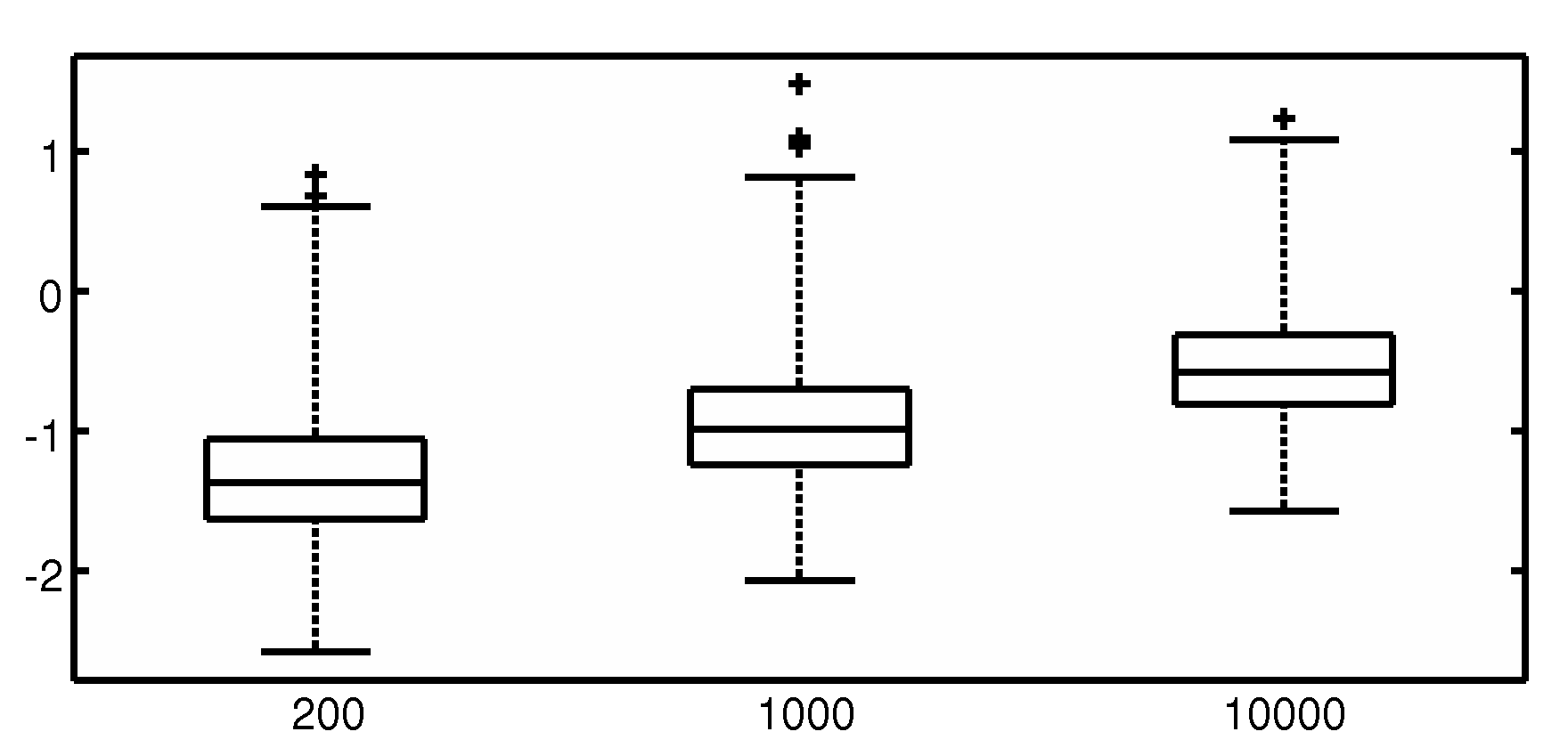
Refer to caption
Fig 3: Boxplots for three different values (n=200,n=1000,n=10.000n=200,\ n=1000,\ n=10.000) of the approximating statistic (37).

In this section we provide further simulation results and discussion to the example from Section 1.1 (cf. also Example 1, Section 3), that is, studying monotonicity of the density ff under Laplace-deconvolution. More precisely, the error density is fϵ(x)=θ−1e−|x|/θf_{\epsilon}(x)=\theta^{-1}e^{-|x|/\theta} with θ=0.075\theta=0.075. In this case,

ℱ⁡(fϵ)​(t)=⟨θ​t⟩−2andop⁡(p)⋆​f=−D​f.\displaystyle\mathcal{F}(f_{\epsilon})(t)=\langle\theta t\rangle^{-2}\quad\text{and}\quad\operatorname{op}(p)^{\star}f=-Df.

One should notice that for Laplace deconvolution the inversion operator, mapping gg to ff, is given by 1−θ2​D21-\theta^{2}D^{2} and therefore the statistic (19) takes the simple form (2) (cf. also the discussion following Theorem 2). The ill-posedness of the shape constraint and the deconvolution problem give m=1m=1, r=2.r=2. Together with (34) it is therefore natural to choose ϕ\phi as the density of a Beta⁡(4,4)\operatorname{Beta}(4,4) random variable. Further, recall that un=1/log⁡log⁡nu_{n}=1/\log\log n, Nn=[n3/5]N_{n}=[n^{3/5}], and

Bn={(kNn,lNn)|k=0,1,…,l=1,2,…,[Nnun],k+l≤Nn}.\displaystyle B_{n}=\Big\{\Big(\frac{k}{N_{n}},\frac{l}{N_{n}}\Big)\ \big|\ k=0,1,\ldots,\ l=1,2,\ldots,[N_{n}u_{n}],\ k+l\leq N_{n}\Big\}.

Note that Assumptions 3 and 4 hold for (A,ρ,r,β0)=(θ2,0,2,2)(A,\rho,r,\beta_{0})=(\theta^{2},0,2,2) and (μ,m)=(1,1)(\mu,m)=(1,1), respectively. Thus, we might work in the framework of Theorem 3. The multiscale statistics

TnP=sup(t,h)∈Bnwh​(|Tt,h−𝔼​Tt,h|g^n​(t)​θ2​‖ϕ(3)‖2−2​log⁡(νh))\displaystyle T_{n}^{P}=\sup_{(t,h)\in B_{n}}w_{h}\left(\frac{|T_{t,h}-\mathbb{E}T_{t,h}|}{\sqrt{\widehat{g}_{n}(t)}\ \theta^{2}\ \|\phi^{(3)}\|_{2}}-\sqrt{2\log\big(\tfrac{\nu}{h}\big)}\right)

and

TnP,∞​(W)=sup(t,h)∈Bnwh​(|∫ϕ(3)​(s−th)​d​Ws|h​‖ϕ(3)‖2−2​log⁡(νh))\displaystyle T_{n}^{P,\infty}(W)=\sup_{(t,h)\in B_{n}}w_{h}\left(\frac{\big|\int\phi^{(3)}\big(\tfrac{s-t}{h}\big)dW_{s}\big|}{\sqrt{h}\ \|\phi^{(3)}\|_{2}}-\sqrt{2\log\big(\tfrac{\nu}{h}\big)}\right) (37)

have a particular simple form as well and the rectangles in (31) can be computed via

dt,hP=h−5/2g^n​(t)θ2∥ϕ(3)∥22​log⁡νh(1+qα,nlog⁡log⁡νhlog⁡νh).\displaystyle d_{t,h}^{P}=h^{-5/2}\sqrt{\widehat{g}_{n}(t)}\theta^{2}\|\phi^{(3)}\|_{2}\sqrt{2\log\tfrac{\nu}{h}}\big(1+q_{\alpha,n}\tfrac{\log\log\tfrac{\nu}{h}}{\log\tfrac{\nu}{h}}\big). (38)

Boxplots for the distributions T200P,∞​(W)T_{200}^{P,\infty}(W), T1000P,∞​(W)T_{1000}^{P,\infty}(W) and T10.000P,∞​(W)T_{10.000}^{P,\infty}(W) are displayed in Figure 3 based on 10.00010.000 repetitions each. The plot shows that the distribution is well-concentrated with a few outliers only. Although our theoretical results imply boundedness of the multiscale statistic as n→∞n\rightarrow\infty, Figure 3 indicates that if nn is in the range of a few thousands TnP,∞​(W)T_{n}^{P,\infty}(W) increases slowly.

Refer to caption
Fig 4: Simulation for sample size n=10.000n=10.000 and 90%90\%-quantile. Upper display: True density ff (dashed) and convoluted density gg (solid). Lower display: Subset of minimal solutions to (i​i)(ii) and (i​i′)(ii^{\prime}) (horizontal lines above/below the thin line)
Refer to caption
Fig 5: True (unobserved) derivative f′f^{\prime} (dashed) and confidence statements for the level of f′f^{\prime}. Computed for the same data set as in Figure 5.

In Section 1.1 we showed confidence statements for a simulated sample of size n=2000n=2000. To complement our study, let us now investigate the case of large nn, i.e. n=10.000n=10.000. Again we choose the confidence level equal to 90%90\%. The estimated quantile is q0.1​(T10.000P,∞​(W))=−0.04q_{0.1}(T_{10.000}^{P,\infty}(W))=-0.04. For all simulations, we use ν=exp⁡(e2)\nu=\exp(e^{2}) because then, h↦log⁡ν/h/(log⁡log⁡ν/h)h\mapsto\sqrt{\log\nu/h}/(\log\log\nu/h) is monotone as long as 0<h≤10<h\leq 1 (cf. Lemma B.11 (i)). The density ff has been designed in order to investigate Corollary 1 numerically. Indeed, on [0,0.35][0,0.35] the signal |f′||f^{\prime}| is large on average, but the intervals on which ff increases/decreases are comparably small. By way of contrast, on [0.35,1][0.35,1] the signal |f′||f^{\prime}| is small and there is only one increase/decrease.

The test is able to find all increases and decreases of ff besides the increase on [0,0.04][0,0.04], which is not detected (cf. Figure 5). In contrast to the simulation in Figure 1, we see now a much better localization of the sharp increase/decrease on [0.2,0.25][0.2,0.25] and [0.25,0.3][0.25,0.3].

With the confidence rectangles at hand, we are able to say more about ff than localizing regions of increase/decrease only. In fact, we also can provide some confidence statements about the value of f′f^{\prime} close to a given point. Instead of plotting all confidence statements, we have displayed in Figure 5 the most prominent ones, allowing for a good characterization of the derivative f′f^{\prime} and telling us something about the strength of the increases/decreases of ff.

A bracket of type “⊔\sqcup” means that f′f^{\prime} has to be above the horizontal line, somewhere. To give an example, from the bracket R​1R1 we can conclude that at least on a subset of [0.07,0.3][0.07,0.3], the derivative f′f^{\prime} exceeds 2929. Similarly, “⊓\sqcap” means that somewhere f′f^{\prime} has to be below the corresponding horizontal line. As always, these statements hold simultaneously with confidence 90%90\%.

What we find is that in regions where the derivative does not oscillate much, we can achieve rather precise confidence statements about the value of f′f^{\prime}. For example, from the rightmost bracket we can infer that with confidence 90%90\% the minimum of f′f^{\prime} on [0.45,1][0.45,1] has to be below −4-4, coming close to the true minimum, which is approximately −6-6.

Figure 5 also shows nicely why a multiscale approach can provide additional insight compared to a one-scale method. Consider R​1R1 and R​2R2 in Figure 5 and denote by (t1,h1)(t_{1},h_{1}) and (t2,h2)(t_{2},h_{2}) the corresponding indices in BnB_{n} (as in (31)). Note that R​1R1 and R​2R2 belong to similar time points in the sense that R​2⊂R​1R2\subset R1 but different bandwidths h1,h2h_{1},h_{2}. Therefore we may view R​1R1 and R​2R2 as a superposition of confidence statements on different scales. This allows to infer different qualitative and quantitative statements close to the same time point. We would use R​2R2 in order to detect and localize an increase (as in Figure 5) or to construct a confidence band for a mode, whereas from R​1R1 we obtain a better lower bound for supf′\sup f^{\prime}. Thus, for a qualitative analysis there is a real gain by taking into account all scales simultaneously.

7 Outlook and Discussion

Given a density deconvolution model, we have investigated multiscale methods in order to analyze qualitative features of the unknown density which can be expressed as pseudo-differential operator inequalities. Compared to previous work, a more refined multiscale calibration has been considered using an idea of proof based on KMT results together with tools from the theory of pseudo-differential operators. We believe that the same strategy can be applied to a variety of other problems. In particular, it is to be expected that similar results will hold for regression and spectral density estimation.

In the formulation of the problem but also in the proofs it becomes apparent that modern tools from functional and harmonic analysis such as pseudo-differential operators are very helpful and to a certain extent unavoidable. In the same spirit, very recently, Nickl and Reiß [40] as well as Söhl and Trabs [43] used singular integral theory in order to prove Donsker theorems in deconvolution-type models. It is expected that reconsidering deconvolution theory from the viewpoint of harmonic analysis will lead to an improved understanding of the field.

Our multiscale approach allows us to identify intervals such that for given significance level we know that op⁡(p)​f>0\operatorname{op}(p)f>0 at least on a subinterval. As outlined in Section 5, these results allow for qualitative inference as for example construction of confidence bands for the roots of op⁡(p)​f\operatorname{op}(p)f. Since we only required that op⁡(p)​f\operatorname{op}(p)f is continuous, op⁡(p)​f\operatorname{op}(p)f can be highly oscillating. In this framework, it is therefore impossible to obtain strong confidence statements in the sense that we find intervals on which op⁡(p)​f\operatorname{op}(p)f is always positive. By adding bias controlling smoothness assumptions such as for instance Hölder conditions stronger results can be obtained resulting for instance in uniform confidence bands.

Obtaining multiscale results for error distributions as in Assumption 2 is already a very difficult topic on its own and extension to the severely ill-posed case, including Gaussian deconvolution, becomes technically challenging since the theory of pseudo-differential operators has to the best of our knowledge not been formulated on the induced function spaces so far. Therefore we intend to treat this in a subsequent paper.

Restricting to shape constraint which are associated with pseudo-differential operators appears to be a limitation of our method, since important shape constraints as for instance curvature cannot be handled within this framework and we may only work with linearizations (which is quite common in physics and engineering). Allowing for non-linearity is a very challenging task for further investigations. We are further aware of the fact that many other important qualitative features are related to integral transforms (that are in general not of convolution type) and they do not have a representation as pseudo-differential operator. For instance complete monotonicity and positive definiteness are by Bernstein’s and Bochner’s Theorem connected to the Laplace transform and Fourier transform, respectively. They cannot be handled with the methods proposed here and are subject to further research.

Acknowledgments. This research was supported by the joint research grant FOR 916 of the German Science Foundation (DFG) and the Swiss National Science Foundation (SNF). The first author was partly funded by DFG postdoctoral fellowship SCHM 2807/1-1. The second author would like to acknowledge support by DFG grants CRC 755 and CRC 803. The authors are grateful for very helpful comments by Steve Marron, Markus Reiß , Jakob Söhl, Mathias Trabs, and Günther Walther as well as two referees and an associate editor which led to a more general version of previous results.

Appendix A Proofs of the main theorems

Throughout the appendix, let

wh=12​log⁡νhlog⁡log⁡νh,w~h=log⁡νhlog⁡log⁡νh.\displaystyle w_{h}=\frac{\sqrt{\tfrac{1}{2}\log\tfrac{\nu}{h}}}{\log\log\tfrac{\nu}{h}},\quad\widetilde{w}_{h}=\frac{\log\tfrac{\nu}{h}}{\log\log\tfrac{\nu}{h}}.

Furthermore, we often use the normalized differential d̸​ξ:=(2​π)−1​d​ξ{\not{d}}\xi:=(2\pi)^{-1}d\xi

Proof of Theorem 1.

In a first step we study convergence of the statistic

Tn(1)=sup(t,h)∈Bnwh​|Tt,h−𝔼​Tt,h|Vt,h​g⁡(t)−w~h.\displaystyle T_{n}^{(1)}=\sup_{(t,h)\in B_{n}}w_{h}\frac{\big|T_{t,h}-\mathbb{E}T_{t,h}\big|}{V_{t,h}\ \sqrt{g(t)}}-\widetilde{w}_{h}.

Note that Tn(1)T_{n}^{(1)} is the same as TnT_{n}, but g^n\widehat{g}_{n} is replaced by the true density gg. We show that there exists a (two-sided) Brownian motion WW, such that with

Tn(2)​(W):=sup(t,h)∈Bnwh​|∫ψt,h​(s)​g⁡(s)​d​Ws|Vt,h​g⁡(t)−w~h,\displaystyle T_{n}^{(2)}(W):=\sup_{(t,h)\in B_{n}}w_{h}\frac{\big|\int\psi_{t,h}(s)\sqrt{g(s)}dW_{s}\big|}{V_{t,h}\ \sqrt{g(t)}}-\widetilde{w}_{h},

we have

supG∈𝒢c,C,q|Tn(1)−Tn(2)​(W)|=oP​(rn).\displaystyle\sup_{G\in\mathcal{G}_{c,C,q}}\big|T_{n}^{(1)}-T_{n}^{(2)}(W)\big|=o_{P}(r_{n}). (39)

The main argument is based on the standard version of KMT (cf. [33]). This is a fairly classical result, but has never been used to describe the asymptotic distribution of a multiscale statistic, the only exception being Walther [44]. In order to state the result, let us define a Brownian bridge on the index set [0,1][0,1] as a centered Gaussian process (B(f)){f∈ℱ},ℱ⊂L2([0,1])(B(f))_{\{f\in\mathcal{F}\}},\ \mathcal{F}\subset L^{2}([0,1]) with covariance structure

Cov⁡(B⁡(f),B⁡(g))=⟨f,g⟩−⟨f,1⟩​⟨g,1⟩.\displaystyle\operatorname{Cov}\big(B(f),B(g)\big)=\langle f,g\rangle-\langle f,1\rangle\langle g,1\rangle.

For ℱ0:={x↦𝕀[0,s]​(x):s∈[0,1]},\mathcal{F}_{0}:=\{x\mapsto\mathbb{I}_{[0,s]}(x):s\in[0,1]\}, the process (B(f)){f∈ℱ0}(B(f))_{\{f\in\mathcal{F}_{0}\}} coincides with the classical definition of a Brownian bridge. If Ui∼𝒰⁡[0,1]U_{i}\sim\mathcal{U}[0,1], i.i.d., the uniform empirical process on the function class ℱ\mathcal{F} is defined as

𝕌n​(f)=n​(1n​∑i=1nf⁡(Ui)−∫f⁡(x)​𝑑x),f∈ℱ.\displaystyle\mathbb{U}_{n}(f)=\sqrt{n}\ \Big(\frac{1}{n}\sum_{i=1}^{n}f(U_{i})-\int f(x)dx\Big),\quad f\in\mathcal{F}.

In particular

Tt,h−𝔼​Tt,h=𝕌n​(ψt,h∘G−1),\displaystyle T_{t,h}-\mathbb{E}\,T_{t,h}=\mathbb{U}_{n}\big(\psi_{t,h}\circ G^{-1}\big),

where G−1G^{-1} denotes the quantile function of YY. For convenience, we restate the celebrated KMT inequality for the uniform empirical process.

Theorem 5 (KMT on [0,1][0,1], cf. [33]).

There exist versions of 𝕌n\mathbb{U}_{n} and a Brownian bridge BB such that for all xx

ℙ(supf∈ℱ0|𝕌n(f)−B(f)|>n−1/2(x+Clogn))<Ke−λ​x,\displaystyle\mathbb{P}\Big(\sup_{f\in\mathcal{F}_{0}}\big|\mathbb{U}_{n}(f)-B(f)\big|>n^{-1/2}(x+C\log n)\Big)<Ke^{-\lambda x},

where C,K,λ>0C,K,\lambda>0 are universal constants.

However, we need a functional version of KMT. We shall prove this by using the theorem above in combination with a result due to Koltchinskii [32], (Theorem 11.4, p. 112) stating that the supremum over a function class ℱ\mathcal{F} behaves as the supremum over the symmetric convex hull sc¯​(ℱ)\overline{\operatorname{sc}}(\mathcal{F}), defined by

sc¯(ℱ):={∑i=1∞λifi:fi∈ℱ,λi∈[−1,1],∑i=1∞|λi|≤1}.\displaystyle\overline{\operatorname{sc}}(\mathcal{F}):=\Big\{\sum_{i=1}^{\infty}\lambda_{i}f_{i}:f_{i}\in\mathcal{F},\lambda_{i}\in[-1,1],\sum_{i=1}^{\infty}|\lambda_{i}|\leq 1\Big\}.
Theorem 6.

Assume there exists a version BB of a Brownian bridge, such that for a sequence (δ~n)n(\widetilde{\delta}_{n})_{n} tending to 00,

ℙ∗​(supf∈ℱ|𝕌n​(f)−B⁡(f)|≥δ~n​(x+C​log⁡n))≤K​e−λ​x,\displaystyle\mathbb{P}^{*}\Big(\sup_{f\in\mathcal{F}}|\mathbb{U}_{n}(f)-B(f)|\geq\widetilde{\delta}_{n}(x+C\log n)\Big)\leq Ke^{-\lambda x},

where C,K,λ>0C,K,\lambda>0 are constants depending only on ℱ\mathcal{F}. Then, there exists a version B~\widetilde{B} of a Brownian bridge, such that

ℙ∗​(supf∈sc¯​(ℱ)|𝕌n​(f)−B~​(f)|≥δ~n​(x+C′​log⁡n))≤K′​e−λ′​x\displaystyle\mathbb{P}^{*}\Big(\sup_{f\in\overline{\operatorname{sc}}(\mathcal{F})}|\mathbb{U}_{n}(f)-\widetilde{B}(f)|\geq\widetilde{\delta}_{n}(x+C^{\prime}\log n)\Big)\leq K^{\prime}e^{-\lambda^{\prime}x}

for constants C′,K′,λ′>0C^{\prime},K^{\prime},\lambda^{\prime}>0.

In Theorem 6, ℙ⋆\mathbb{P}^{\star} refers to the outer measure, however, for the function class considered in this paper, we have measurability of the corresponding event and hence may replace ℙ⋆\mathbb{P}^{\star} by ℙ\mathbb{P}. It is well-known (cf. Giné et al. [19], p. 172) that

{ρ|ρ:ℝ→ℝ,suppρ⊂[0,1],ρ(1)=0,TV(ρ)≤1}⊂sc¯(ℱ0).\displaystyle\big\{\rho\ \big|\ \rho:\mathbb{R}\rightarrow\mathbb{R},\ \operatorname{supp}\rho\subset[0,1],\ \rho(1)=0,\ \operatorname{TV}(\rho)\leq 1\big\}\subset\overline{\operatorname{sc}}(\mathcal{F}_{0}). (40)

Now, assume that ρ:ℝ→ℝ\rho:\mathbb{R}\rightarrow\mathbb{R} is such that TV⁡(ρ)+3​|ρ⁡(1)|≤1\operatorname{TV}(\rho)+3|\rho(1)|\leq 1. Define ρ~=(ρ−ρ⁡(1)​𝕀[0,1])/(1−|ρ⁡(1)|)\widetilde{\rho}=(\rho-\rho(1)\mathbb{I}_{[0,1]})/(1-|\rho(1)|) and observe that TV⁡(ρ~)≤1\operatorname{TV}(\widetilde{\rho})\leq 1 and ρ~​(1)=0\widetilde{\rho}(1)=0. By (40) there exists λ1,λ2,…∈ℝ\lambda_{1},\lambda_{2},\ldots\in\mathbb{R} and t1,t2,…∈[0,1]t_{1},t_{2},\ldots\in[0,1] such that ρ~=∑λi​𝕀[0,ti]\widetilde{\rho}=\sum\lambda_{i}\mathbb{I}_{[0,t_{i}]} and ∑|λi|≤1\sum|\lambda_{i}|\leq 1. Therefore, ρ=(1−|ρ⁡(1)|)​ρ~+ρ⁡(1)​𝕀[0,1]\rho=(1-|\rho(1)|)\widetilde{\rho}+\rho(1)\mathbb{I}_{[0,1]} can be written as linear combination of indicator functions, such that the sum of the absolute values of weights is bounded by 11. This shows

{ρ|ρ:ℝ→ℝ,suppρ⊂[0,1],TV(ρ)+3|ρ(1)|≤1}⊂sc¯(ℱ0).\displaystyle\big\{\rho\ \big|\ \rho:\mathbb{R}\rightarrow\mathbb{R},\ \operatorname{supp}\rho\subset[0,1],\ \operatorname{TV}(\rho)+3|\rho(1)|\leq 1\big\}\subset\overline{\operatorname{sc}}(\mathcal{F}_{0}).

Since TV⁡(ψt,h∘G−1)≤TV⁡(ψt,h)\operatorname{TV}(\psi_{t,h}\circ G^{-1})\leq\operatorname{TV}(\psi_{t,h}) it follows by Assumption 1 (ii) that the function class

ℱn:={C⋆Vt,h−1hψt,h∘G−1:(t,h)∈Bn,G∈𝒢c,C,q}\displaystyle\mathcal{F}_{n}:=\Big\{C_{\star}V_{t,h}^{-1}\sqrt{h}\ \psi_{t,h}\circ G^{-1}:(t,h)\in B_{n},\ G\in\mathcal{G}_{c,C,q}\Big\}

is a subset of sc¯​(ℱ0)\overline{\operatorname{sc}}(\mathcal{F}_{0}) for sufficiently small constant C⋆C_{\star}. Combining Theorems 5 and 6 shows for δ~n=n−1/2\widetilde{\delta}_{n}=n^{-1/2} that there are constants C′,K′,λ′C^{\prime},K^{\prime},\lambda^{\prime} and a Brownian bridge (B⁡(f))f∈sc¯​(ℱ0)(B(f))_{f\in\overline{\operatorname{sc}}(\mathcal{F}_{0})} such that for x>0x>0, the probability of

{sup(t,h)∈Bn,G∈𝒢C⋆h​|𝕌n​(ψt,h∘G−1)−B⁡(ψt,h∘G−1)|Vt,h≥1n(x+C′logn)}\displaystyle\Big\{\sup_{(t,h)\in B_{n},\ G\in\mathcal{G}}C_{\star}\frac{\sqrt{h}\big|\mathbb{U}_{n}\big(\psi_{t,h}\circ G^{-1}\big)-B\big(\psi_{t,h}\circ G^{-1}\big)\big|}{V_{t,h}}\geq\frac{1}{\sqrt{n}}(x+C^{\prime}\log n)\Big\}

is bounded by K′​e−λ′​xK^{\prime}e^{-\lambda^{\prime}x}. Due to Lemma B.11 (i) and ln≥ν/nl_{n}\geq\nu/n for sufficiently large nn, we have that wln≤wν/nw_{l_{n}}\leq w_{\nu/n}. This readily implies with x=log⁡nx=\log n that

sup(t,h)∈Bn,G∈𝒢wh​||Tt,h−𝔼​Tt,h|−|B⁡(ψt,h∘G−1)||Vt,h​g⁡(t)=OP​(1ln​n​wν/n​log⁡n).\displaystyle\sup_{(t,h)\in B_{n},\ G\in\mathcal{G}}w_{h}\frac{\Big|\big|T_{t,h}-\mathbb{E}\,T_{t,h}\big|-\big|B\big(\psi_{t,h}\circ G^{-1}\big)\big|\Big|}{V_{t,h}\ \sqrt{g(t)}}=O_{P}\Big(\frac{1}{\sqrt{l_{n}n}}w_{\nu/n}\log n\Big).

Now, let us introduce the (general) Brownian motion W⁡(f)W(f) as a centered Gaussian process with covariance 𝔼⁡[W⁡(f)​W​(g)]=⟨f,g⟩\mathbb{E}[W(f)W(g)]=\langle f,g\rangle. In particular, W⁡(f)=B⁡(f)+(∫f)​ξW(f)=B(f)+(\int f)\xi, ξ∼𝒩⁡(0,1)\xi\sim\mathcal{N}(0,1) and independent of BB, defines a Brownian motion and hence there exists a version of (W⁡(f))f∈sc¯​(ℱ0)(W(f))_{f\in\overline{\operatorname{sc}}(\mathcal{F}_{0})} such that B⁡(f)=W⁡(f)−(∫f)​W​(1)B(f)=W(f)-(\int f)W(1). We have

sup(t,h)∈Bn,G∈𝒢wh​|∫ψt,h​(u)​𝑑G​(u)|Vt,h​g⁡(t)\displaystyle\sup_{(t,h)\in B_{n},\ G\in\mathcal{G}}w_{h}\frac{\big|\int\psi_{t,h}(u)\ dG(u)\big|}{V_{t,h}\ \sqrt{g(t)}} ≤c−1​sup(t,h)∈Bn,G∈𝒢wh​‖ψt,h‖1Vt,h​g⁡(t)\displaystyle\leq c^{-1}\sup_{(t,h)\in B_{n},\ G\in\mathcal{G}}w_{h}\frac{\|\psi_{t,h}\|_{1}}{V_{t,h}\ \sqrt{g(t)}}
≲suph∈[ln,un]wh​h1/2≤wun​un1/2,\displaystyle\lesssim\sup_{h\in[l_{n},u_{n}]}w_{h}h^{1/2}\leq w_{u_{n}}u_{n}^{1/2},

where the second inequality follows from Assumption 1 (ii) and the last inequality from Lemma B.11 (ii). This implies further

𝔼⁡[‖whVt,h​g⁡(t)​[|B⁡(ψt,h∘G−1)|−|W⁡(ψt,h∘G−1)|]‖ℱn]=O⁡(wun​un1/2),\displaystyle\mathbb{E}\Big[\Big\|\frac{w_{h}}{V_{t,h}\ \sqrt{g(t)}}\Big[\big|B\big(\psi_{t,h}\circ G^{-1}\big)\big|-\big|W\big(\psi_{t,h}\circ G^{-1}\big)\big|\Big]\Big\|_{\mathcal{F}_{n}}\Big]=O(w_{u_{n}}u_{n}^{1/2}),

and therefore

supG∈𝒢|Tn(1)−sup(t,h)∈Bnwh​|W⁡(ψt,h∘G−1)|Vt,h​g⁡(t)−w~h|=OP​(w1/n​log⁡nln​n+wun​un1/2),\displaystyle\sup_{G\in\mathcal{G}}\Big|T_{n}^{(1)}-\sup_{(t,h)\in B_{n}}w_{h}\frac{\big|W\big(\psi_{t,h}\circ G^{-1}\big)\big|}{V_{t,h}\ \sqrt{g(t)}}-\widetilde{w}_{h}\Big|=O_{P}(\frac{w_{1/n}\log n}{\sqrt{l_{n}n}}+w_{u_{n}}u_{n}^{1/2}),

and

supG∈𝒢|Tn(1)−Tn(2)(W)|=OP(ln−1/2n−1/2w1/nlogn+wunun1/2).\displaystyle\sup_{G\in\mathcal{G}}\Big|T_{n}^{(1)}-T_{n}^{(2)}(W)\Big|=O_{P}(l_{n}^{-1/2}n^{-1/2}w_{1/n}\log n+w_{u_{n}}u_{n}^{1/2}).

In the last equality we used that (Wt(1))t∈[0,1]=(W⁡(𝕀[0,t]​(⋅)))t∈[0,1](W^{(1)}_{t})_{t\in[0,1]}=(W(\mathbb{I}_{[0,t]}(\cdot)))_{t\in[0,1]} and

(Wt)t∈ℝ=(∫0t𝕀{g>0}(s)g⁡(s)​d​WG⁡(s)(1))t∈ℝ(W_{t})_{t\in\mathbb{R}}=\Big(\int_{0}^{t}\frac{\mathbb{I}_{\{g>0\}}(s)}{\sqrt{g(s)}}dW_{G(s)}^{(1)}\Big)_{t\in\mathbb{R}}

are (two-sided) standard Brownian motions, proving W⁡(ψt,h∘G−1)=∫ψt,h​(s)​g⁡(s)​d​WsW(\psi_{t,h}\circ G^{-1})=\linebreak\int\psi_{t,h}(s)\sqrt{g(s)}dW_{s} and hence (39). Further note that Assumption 1 (iii) together with Lemma B.10 shows that

supG∈𝒢|Tn(2)​(W)−sup(t,h)∈Bnwh​|∫ψt,h​(s)​d​Ws|Vt,h−w~h|=OP​(κn).\displaystyle\sup_{G\in\mathcal{G}}\Big|T_{n}^{(2)}(W)-\sup_{(t,h)\in B_{n}}w_{h}\frac{\big|\int\psi_{t,h}(s)dW_{s}\big|}{V_{t,h}}-\widetilde{w}_{h}\Big|=O_{P}(\kappa_{n}).

In a final step let us show that (13) is almost surely bounded. In order to establish the result, we use Theorem 6.1 and Remark 1 of Dümbgen and Spokoiny [13]. We set ρ⁡((t,h),(t′,h′))=(|t−t′|+|h−h′|)1/2\rho\big((t,h),(t^{\prime},h^{\prime})\big)=(|t-t^{\prime}|+|h-h^{\prime}|)^{1/2}. Further, let X⁡(t,h)=h​Vt,h−1​∫ψt,h​(s)​d​WsX(t,h)=\sqrt{h}V_{t,h}^{-1}\int\psi_{t,h}(s)dW_{s} and σ⁡(t,h)=h1/2\sigma(t,h)=h^{1/2}.

By assumption, XX has continuous sample paths on 𝒯\mathcal{T} and obviously, for all (t,h),(t′,h′)∈𝒯(t,h),(t^{\prime},h^{\prime})\in\mathcal{T},

σ2​(t,h)≤σ2​(t′,h′)+ρ2​((t,h),(t′,h′)).\displaystyle\sigma^{2}(t,h)\leq\sigma^{2}(t^{\prime},h^{\prime})+\rho^{2}((t,h),(t^{\prime},h^{\prime})).

Let Z∼𝒩⁡(0,1)Z\sim\mathcal{N}(0,1). Since X⁡(t,h)X(t,h) is a Gaussian process and Vt,h≥‖ϕt,h‖2V_{t,h}\geq\|\phi_{t,h}\|_{2}, ℙ(X(t,h)>σ(t,h)η)≤ℙ(Z>η)≤exp(−η2/2)\mathbb{P}(X(t,h)>\sigma(t,h)\eta)\leq\mathbb{P}(Z>\eta)\leq\exp(-\eta^{2}/2) for any η>0\eta>0. Further, denote by

At,t′,h,h′:=‖ψt,h​hVt,h−ψt′,h′​h′Vt′,h′‖2.\displaystyle A_{t,t^{\prime},h,h^{\prime}}:=\left\|\frac{\psi_{t,h}\sqrt{h}}{V_{t,h}}-\frac{\psi_{t^{\prime},h^{\prime}}\sqrt{h}^{\prime}}{V_{t^{\prime},h^{\prime}}}\right\|_{2}. (41)

Because of ℙ(|X(t,h)−X(t′,h′)|≥At,t′,h,h′η)≤2exp(−η2/2)\mathbb{P}(|X(t,h)-X(t^{\prime},h^{\prime})\big|\geq A_{t,t^{\prime},h,h^{\prime}}\eta\Big)\leq 2\exp\big(-\eta^{2}/2\big) we have by Lemma B.6 for a universal constant K>0K>0,

ℙ(|X(t,h)−X(t′,h′)|≥ρ((t,h),(t′,h′))η)≤2exp(−η2/(2K2)).\displaystyle\mathbb{P}\Big(\big|X(t,h)-X(t^{\prime},h^{\prime})\big|\geq\rho((t,h),(t^{\prime},h^{\prime}))\eta\Big)\leq 2\exp\big(-\eta^{2}/(2K^{2})\big).

Finally, we can bound the entropy 𝒩⁡((δ​u)1/2,{(t,h)∈𝒯:h≤δ})\mathcal{N}((\delta u)^{1/2},\{(t,h)\in\mathcal{T}:h\leq\delta\}) similarly as in [13], p. 145. Therefore, application of Remark 1 in [13] shows that

S:=sup(t,h)∈𝒯12​log⁡eh​|∫ψt,h​(s)​d​Ws|log⁡(e​log⁡eh)​Vt,h−log⁡(1h)​log⁡(eh)log⁡(e​log⁡eh)\displaystyle S:=\sup_{(t,h)\in\mathcal{T}}\frac{\sqrt{\tfrac{1}{2}\log\tfrac{e}{h}}\ \big|\int\psi_{t,h}(s)dW_{s}\big|}{\log\big(e\log\tfrac{e}{h}\big)\ V_{t,h}}-\frac{\sqrt{\log(\tfrac{1}{h})\log(\tfrac{e}{h})}}{\log\big(e\log\tfrac{e}{h}\big)}

is almost surely bounded from above. Define

S′:=sup(t,h)∈𝒯12​log⁡νh​|∫ψt,h​(s)​d​Ws|log⁡log​νh​Vt,h−log⁡(1h)​log⁡(νh)log⁡log⁡νh.\displaystyle S^{\prime}:=\sup_{(t,h)\in\mathcal{T}}\frac{\sqrt{\tfrac{1}{2}\log\tfrac{\nu}{h}}\ \big|\int\psi_{t,h}(s)dW_{s}\big|}{\log\log\tfrac{\nu}{h}\ V_{t,h}}-\frac{\sqrt{\log(\tfrac{1}{h})\log(\tfrac{\nu}{h})}}{\log\log\tfrac{\nu}{h}}.

If e<ν≤eee<\nu\leq e^{e}, then

log⁡log⁡νh=log⁡(log⁡νe​log⁡eehe/log⁡ν)≥log⁡log⁡ν−1+log⁡(e​log​eh)\displaystyle\log\log\tfrac{\nu}{h}=\log\Big(\tfrac{\log\nu}{e}\log\tfrac{e^{e}}{h^{e/\log\nu}}\Big)\geq\log\log\nu-1+\log\big(e\log\tfrac{e}{h}\big)

implies

log⁡(e​log⁡eh)log⁡log⁡νh≤1log⁡log⁡ν+1.\displaystyle\frac{\log\big(e\log\tfrac{e}{h}\big)}{\log\log\tfrac{\nu}{h}}\leq\frac{1}{\log\log\nu}+1.

Furthermore, log⁡ν/h≤(log⁡ν)​(log⁡e/h)\log\nu/h\leq(\log\nu)(\log e/h). Suppose now that S′>0S^{\prime}>0 (otherwise S′S^{\prime} is bounded from below by 00). Then, S′≲SS^{\prime}\lesssim S and hence S′S^{\prime} is almost surely bounded. Finally,

log⁡νh​|log⁡1h−log⁡νh|≤log⁡ν.\displaystyle\sqrt{\log\tfrac{\nu}{h}}\big|\sqrt{\log\tfrac{1}{h}}-\sqrt{\log\tfrac{\nu}{h}}\big|\leq\log\nu.

Therefore, (13) holds, i.e.

sup(t,h)∈𝒯wh​|∫ψt,h​(s)​d​Ws|Vt,h−w~h\displaystyle\sup_{(t,h)\in\mathcal{T}}w_{h}\frac{\big|\int\psi_{t,h}(s)dW_{s}\big|}{V_{t,h}}-\widetilde{w}_{h}

is almost surely bounded.

In the last step, it remains to prove that supG∈𝒢c,C,q|Tn−Tn(1)|=OP​(supG∈𝒢‖g^n−g‖∞​log⁡n/log⁡log⁡n)\sup_{G\in\mathcal{G}_{c,C,q}}|T_{n}-T_{n}^{(1)}|=O_{P}(\sup_{G\in\mathcal{G}}\|\widehat{g}_{n}-g\|_{\infty}\log n/\log\log n). For sufficiently large nn and because G∈𝒢G\in\mathcal{G}, g^n≥c/2\widehat{g}_{n}\geq c/2 for all t∈[0,1]t\in[0,1]. Therefore using Lemma B.11 (i),

supG∈𝒢|Tn−Tn(1)|\displaystyle\sup_{G\in\mathcal{G}}\big|T_{n}-T_{n}^{(1)}| ≤sup(t,h)∈Bn,G∈𝒢wh​|Tt,h−𝔼⁡[Tt,h]|Vt,h​g⁡(t)​supG∈𝒢‖g^n−g‖∞g^n​(t)\displaystyle\leq\sup_{(t,h)\in B_{n},\ G\in\mathcal{G}}w_{h}\frac{\big|T_{t,h}-\mathbb{E}[T_{t,h}]\big|}{V_{t,h}\ \sqrt{g(t)}}\frac{\sup_{G\in\mathcal{G}}\big\|\widehat{g}_{n}-g\big\|_{\infty}}{\widehat{g}_{n}(t)}
≤2​supG∈𝒢‖g^n−g‖∞c​sup(t,h)∈Bn,G∈𝒢wh​|Tt,h−𝔼⁡[Tt,h]|Vt,h​g⁡(t)\displaystyle\leq\frac{2\sup_{G\in\mathcal{G}}\big\|\widehat{g}_{n}-g\big\|_{\infty}}{c}\sup_{(t,h)\in B_{n},\ G\in\mathcal{G}}w_{h}\frac{\big|T_{t,h}-\mathbb{E}[T_{t,h}]\big|}{V_{t,h}\ \sqrt{g(t)}}
≤2​supG∈𝒢‖g^n−g‖∞c​(Tn(1)+suph∈[ln,un]w~h)\displaystyle\leq\frac{2\sup_{G\in\mathcal{G}}\big\|\widehat{g}_{n}-g\big\|_{\infty}}{c}(T_{n}^{(1)}+\sup_{h\in[l_{n},u_{n}]}\widetilde{w}_{h})
≤2​supG∈𝒢‖g^n−g‖∞c​(Tn(1)+O⁡(log⁡nlog⁡log⁡n)).\displaystyle\leq\frac{2\sup_{G\in\mathcal{G}}\big\|\widehat{g}_{n}-g\big\|_{\infty}}{c}\big(T_{n}^{(1)}+O(\frac{\log n}{\log\log n})\big). (42)

Since Tn(1)T_{n}^{(1)} is a.s. bounded by Theorem 1, the result follows. ∎

Remark 1.

Next, we give a proof of Theorem 2. In fact we proof a slightly stronger version, which does not necessarily require the symbol aa to be elliptic and Vt,h=‖vt,h‖2V_{t,h}=\|v_{t,h}\|_{2}. It is only assumed that

  • (i)

    Vt,h≥‖vt,h‖2V_{t,h}\geq\|v_{t,h}\|_{2},

  • (ii)

    there exists constants cV,CVc_{V},C_{V} with 0<cV≤hm+r−1/2​Vt,h≤CV<∞0<c_{V}\leq h^{m+r-1/2}V_{t,h}\leq C_{V}<\infty

  • (iii)

    for all (t,h),(t′,h′)∈𝒯(t,h),(t^{\prime},h^{\prime})\in\mathcal{T} and whenever h≤h′h\leq h^{\prime} it holds that hm+r​|Vt,h−Vt′,h′|≤CV​(|t−t′|+|h−h′|)1/2h^{m+r}|V_{t,h}-V_{t^{\prime},h^{\prime}}|\leq C_{V}(|t-t^{\prime}|+|h-h^{\prime}|)^{1/2}.

As a special case these conditions are satisfied for Vt,h=‖vt,h‖2V_{t,h}=\|v_{t,h}\|_{2} and op⁡(a)\operatorname{op}(a) elliptic. This follows directly from Lemmas B.3 and B.5.

Proof of Theorem 2.

In order to prove the statements it is sufficient to check the conditions of Theorem 1. For h>0h>0 define the symbol

at,h⋆​(x,ξ):=hm¯​a⋆​(x​h+t,h−1​ξ).\displaystyle a_{t,h}^{\star}(x,\xi):=h^{\overline{m}}a^{\star}(xh+t,h^{-1}\xi). (43)

Under the imposed conditions and by Remark B.1 we may apply Lemma B.2 for 𝔞(t,h)=at,h⋆\mathfrak{a}^{(t,h)}=a_{t,h}^{\star} and therefore, uniformly over (t,h)∈𝒯(t,h)\in\mathcal{T} and u,u′∈ℝu,u^{\prime}\in\mathbb{R},

  • (I)

    |vt,h​(u)|≲h−m−r​min⁡(1,h2(u−t)2)|v_{t,h}(u)|\lesssim h^{-m-r}\min\big(1,\tfrac{h^{2}}{(u-t)^{2}}\big).

  • (II)

    |vt,h​(u)−vt,h​(u′)|≲h−m−r−1​|u−u′||v_{t,h}(u)-v_{t,h}(u^{\prime})|\lesssim h^{-m-r-1}|u-u^{\prime}| and if u,u′≠tu,u^{\prime}\neq t,

    |vt,h​(u)−vt,h​(u′)|≲h1−m−r​|u−u′||u′−t|​|u−t|=h1−m−r​|∫u′u1(x−t)2​𝑑x|.|v_{t,h}(u)-v_{t,h}(u^{\prime})|\lesssim h^{1-m-r}\frac{|u-u^{\prime}|}{|u^{\prime}-t|\ |u-t|}=h^{1-m-r}\big|\int_{u^{\prime}}^{u}\frac{1}{(x-t)^{2}}dx\big|.

Using (I), we obtain ‖vt,h‖∞≲h−m−r\|v_{t,h}\|_{\infty}\lesssim h^{-m-r} and ‖vt,h‖1≲h1−m−r\|v_{t,h}\|_{1}\lesssim h^{1-m-r}. In order to show that the total variation is of the right order, let us decompose vt,hv_{t,h} further into vt,h(1)=vt,h​𝕀[t−h,t+h]v_{t,h}^{(1)}=v_{t,h}\mathbb{I}_{[t-h,t+h]} and vt,h(2)=vt,h−vt,h(1)v_{t,h}^{(2)}=v_{t,h}-v_{t,h}^{(1)}. By (II), TV⁡(vt,h(1))≲h−m−r\operatorname{TV}(v_{t,h}^{(1)})\lesssim h^{-m-r} and

TV⁡(vt,h(2))≲h−m−r+h1−m−r​∫t+h∞1(x−t)2​𝑑x≲h−m−r.\displaystyle\operatorname{TV}(v_{t,h}^{(2)})\lesssim h^{-m-r}+h^{1-m-r}\int_{t+h}^{\infty}\frac{1}{(x-t)^{2}}dx\lesssim h^{-m-r}.

Since TV⁡(vt,h)≤TV⁡(vt,h(1))+TV⁡(vt,h(2))≲h−m−r\operatorname{TV}(v_{t,h})\leq\operatorname{TV}(v_{t,h}^{(1)})+\operatorname{TV}(v_{t,h}^{(2)})\lesssim h^{-m-r}, this shows together with Remark 1 that part (ii) of Assumption 1 is satisfied.

Next, we verify Assumption 1, (iii) with κn=sup(t,h)∈Bnwh​h1/2​log⁡(1/h)≲un1/2​log3/2​n\kappa_{n}=\sup_{(t,h)\in B_{n}}w_{h}h^{1/2}\log(1/h)\lesssim u_{n}^{1/2}\log^{3/2}n (cf. Lemma B.11, (ii)), i.e. we show

sup(t,h)∈Bn,G∈𝒢wh​TV⁡(vt,h​(⋅)​[g⁡(⋅)−g⁡(t)]​⟨⋅⟩α)Vt,h≲un1/2​log3/2​n.\displaystyle\sup_{(t,h)\in B_{n},\ G\in\mathcal{G}}w_{h}\frac{\operatorname{TV}\big(v_{t,h}(\cdot)[\sqrt{g(\cdot)}-\sqrt{g(t)}]\langle\cdot\rangle^{\alpha}\big)}{V_{t,h}}\lesssim u_{n}^{1/2}\log^{3/2}n.

By Lemma B.12, we see that this holds for vt,hv_{t,h} replaced by vt,h(1)v_{t,h}^{(1)}. Therefore, it remains to prove the statement for vt,h(2)v_{t,h}^{(2)}. Let us decompose vt,h(2)v_{t,h}^{(2)} further into vt,h(2,1)=vt,h​𝕀[t−1,t+1]∩[t−h,t+h]cv_{t,h}^{(2,1)}=v_{t,h}\mathbb{I}_{[t-1,t+1]\cap[t-h,t+h]^{c}} and vt,h(2,2)=vt,h(2)−vt,h(2,1)=vt,h​𝕀[t−1,t+1]cv_{t,h}^{(2,2)}=v_{t,h}^{(2)}-v_{t,h}^{(2,1)}=v_{t,h}\mathbb{I}_{[t-1,t+1]^{c}}. For the remaining part, let u,u′u,u^{\prime} be such that |u−t|≥|u′−t|≥h|u-t|\geq|u^{\prime}-t|\geq h. We have

TV⁡(vt,h(2,1)​(⋅)​[g⁡(⋅)−g⁡(t)]​⟨⋅⟩α)\displaystyle\operatorname{TV}\big(v_{t,h}^{(2,1)}(\cdot)\big[\sqrt{g(\cdot)}-\sqrt{g(t)}\big]\langle\cdot\rangle^{\alpha}\big) ≲‖vt,h(2,1)​(⋅)​[g⁡(⋅)−g⁡(t)]‖∞\displaystyle\lesssim\big\|v_{t,h}^{(2,1)}(\cdot)\big[\sqrt{g(\cdot)}-\sqrt{g(t)}\big]\big\|_{\infty}
+TV⁡(vt,h(2,1)​(⋅)​[g⁡(⋅)−g⁡(t)]).\displaystyle\quad+\operatorname{TV}\big(v_{t,h}^{(2,1)}(\cdot)\big[\sqrt{g(\cdot)}-\sqrt{g(t)}\big]\big). (44)

Using (I) and (II) together with the properties of the class 𝒢\mathcal{G} we can bound the variation |vt,h(2,1)​(u)​[g⁡(u)−g⁡(t)]−vt,h(2,1)​(u′)​[g⁡(u′)−g⁡(t)]|\big|v_{t,h}^{(2,1)}(u)\big[\sqrt{g(u)}-\sqrt{g(t)}\big]-v_{t,h}^{(2,1)}(u^{\prime})\big[\sqrt{g(u^{\prime})}-\sqrt{g(t)}\big]\big| by

|vt,h(2,1)​(u)−vt,h(2,1)​(u′)|⋅|g⁡(u′)−g⁡(t)|+|vt,h(2,1)​(u)|⋅|g⁡(u)−g⁡(u′)|\displaystyle\big|v_{t,h}^{(2,1)}(u)-v_{t,h}^{(2,1)}(u^{\prime})\big|\cdot\big|\sqrt{g(u^{\prime})}-\sqrt{g(t)}\big|+\big|v_{t,h}^{(2,1)}(u)\big|\cdot\big|\sqrt{g(u)}-\sqrt{g(u^{\prime})}\big|
≲h1−m−r​|u−u′||u−t|+h2−m−r​|u−u′||u−t|2≲h1−m−r​|u−u′||u−t|≤h1−m−r​|∫u′u1|x−t|​𝑑x|.\displaystyle\lesssim h^{1-m-r}\tfrac{|u-u^{\prime}|}{|u-t|}+h^{2-m-r}\tfrac{|u-u^{\prime}|}{|u-t|^{2}}\lesssim h^{1-m-r}\tfrac{|u-u^{\prime}|}{|u-t|}\leq h^{1-m-r}\big|\int_{u^{\prime}}^{u}\tfrac{1}{|x-t|}dx\big|.

Due to h≥ln≳1/nh\geq l_{n}\gtrsim 1/n this yields

TV⁡(vt,h(2,1)​(⋅)​[g⁡(⋅)−g⁡(t)])\displaystyle\operatorname{TV}\big(v_{t,h}^{(2,1)}(\cdot)[\sqrt{g(\cdot)}-\sqrt{g(t)}]\big) ≲h1−m−r+h1−m−r​∫t+ht+1d​u|u−t|\displaystyle\lesssim h^{1-m-r}+h^{1-m-r}\int_{t+h}^{t+1}\frac{du}{|u-t|}
≲h1−m−r​log⁡1h≲h1−m−r​log⁡n\displaystyle\lesssim h^{1-m-r}\log\tfrac{1}{h}\lesssim h^{1-m-r}\log n

and with (44) also

TV⁡(vt,h(2,1)​(⋅)​[g⁡(⋅)−g⁡(t)]​⟨⋅⟩α)≲h1−m−r​log⁡n.\displaystyle\operatorname{TV}\big(v_{t,h}^{(2,1)}(\cdot)\big[\sqrt{g(\cdot)}-\sqrt{g(t)}\big]\langle\cdot\rangle^{\alpha}\big)\lesssim h^{1-m-r}\log n. (45)

Finally, let us address the total variation term involving vt,h(2,2)v_{t,h}^{(2,2)}. Given 𝒢c,C,q\mathcal{G}_{c,C,q} we can choose α\alpha such that α>1/2\alpha>1/2 and α+q<1\alpha+q<1 (recall that 0≤q<1/20\leq q<1/2). By Lemma B.7, we find that

|vt,h(2,2)​(u)​⟨u⟩α−vt,h(2,2)​(u′)​⟨u′⟩α|\displaystyle\big|v_{t,h}^{(2,2)}(u)\langle u\rangle^{\alpha}-v_{t,h}^{(2,2)}(u^{\prime})\langle u^{\prime}\rangle^{\alpha}\big| ≲h1−m−r​|∫u′u1(x−t)2−α+1(x−t)2​𝑑x|.\displaystyle\lesssim h^{1-m-r}\Big|\int_{u^{\prime}}^{u}\frac{1}{(x-t)^{2-\alpha}}+\frac{1}{(x-t)^{2}}dx\Big|.

Moreover

⟨u⟩α​(1+|u′|+|u|)q\displaystyle\langle u\rangle^{\alpha}(1+|u^{\prime}|+|u|)^{q} ≤(1+|u′|+|u|)q+α\displaystyle\leq(1+|u^{\prime}|+|u|)^{q+\alpha}
≤(3+2​|u−t|)q+α≤3+2​|u−t|q+α\displaystyle\leq(3+2|u-t|)^{q+\alpha}\leq 3+2|u-t|^{q+\alpha}

and thus

|vt,h(2,2)​(u)​⟨u⟩α|​|g⁡(u)−g⁡(u′)|≲h2−m−r​|u−t|q+α+1|u−t|2​|u−u′|.\displaystyle\big|v_{t,h}^{(2,2)}(u)\langle u\rangle^{\alpha}\big|\ \big|\sqrt{g(u)}-\sqrt{g(u^{\prime})}\big|\lesssim h^{2-m-r}\frac{|u-t|^{q+\alpha}+1}{|u-t|^{2}}|u-u^{\prime}|.

This allows us to bound the variation by

|vt,h(2,2)​(u)​[g⁡(u)−g⁡(t)]​⟨u⟩α−vt,h(2,2)​(u′)​[g⁡(u′)−g⁡(t)]​⟨u′⟩α|\displaystyle\big|v_{t,h}^{(2,2)}(u)\big[\sqrt{g(u)}-\sqrt{g(t)}\big]\langle u\rangle^{\alpha}-v_{t,h}^{(2,2)}(u^{\prime})\big[\sqrt{g(u^{\prime})}-\sqrt{g(t)}\big]\langle u^{\prime}\rangle^{\alpha}\big|
≤|vt,h(2,2)​(u)​⟨u⟩α|​|g⁡(u)−g⁡(u′)|+2c​|vt,h(2,2)​(u)​⟨u⟩α−vt,h(2,2)​(u′)​⟨u′⟩α|\displaystyle\leq\big|v_{t,h}^{(2,2)}(u)\langle u\rangle^{\alpha}\big|\ \big|\sqrt{g(u)}-\sqrt{g(u^{\prime})}\big|+\frac{2}{\sqrt{c}}\big|v_{t,h}^{(2,2)}(u)\langle u\rangle^{\alpha}-v_{t,h}^{(2,2)}(u^{\prime})\langle u^{\prime}\rangle^{\alpha}\big|
≲h1−m−r​|∫u′u1(x−t)2−q−α+1(x−t)2−α+1(x−t)2​𝑑x|\displaystyle\lesssim h^{1-m-r}\Big|\int_{u^{\prime}}^{u}\frac{1}{(x-t)^{2-q-\alpha}}+\frac{1}{(x-t)^{2-\alpha}}+\frac{1}{(x-t)^{2}}\ dx\ \Big|

and therefore we conclude that

TV⁡(vt,h(2,2)​(⋅)​[g⁡(⋅)−g⁡(t)]​⟨⋅⟩α)\displaystyle\operatorname{TV}\big(v_{t,h}^{(2,2)}(\cdot)\big[\sqrt{g(\cdot)}-\sqrt{g(t)}\big]\langle\cdot\rangle^{\alpha}\big)
≲h1−m−r+h1−m−r​∫t+1∞1(x−t)2−q−α+1(x−t)2−α+1(x−t)2​𝑑x\displaystyle\lesssim h^{1-m-r}+h^{1-m-r}\int_{t+1}^{\infty}\frac{1}{(x-t)^{2-q-\alpha}}+\frac{1}{(x-t)^{2-\alpha}}+\frac{1}{(x-t)^{2}}dx
≤h1−m−r.\displaystyle\leq h^{1-m-r}.

Together with the bound for vt,h(1)v_{t,h}^{(1)} and (45) this yields Assumption 1, (iii).

Finally, Assumption 1 (iv) follows from Lemma B.5 and Remark 1 due to ϕ∈H⌈r+m⌉∩Hr+m+1/2\phi\in H^{\lceil r+m\rceil}\cap H^{r+m+1/2}, supp⁡ϕ⊂[0,1]\operatorname{supp}\phi\subset[0,1] and ϕ∈TV⁡(D⌈r+m⌉​ϕ)<∞\phi\in\operatorname{TV}(D^{\lceil r+m\rceil}\phi)<\infty. This shows that Assumption 1 holds for (vt,h,Vt,h)(v_{t,h},V_{t,h}).

In the next step, we verify that (t,h)↦X⁡(t,h)=h​Vt,h−1​∫vt,h​(s)​d​Ws(t,h)\mapsto X(t,h)=\sqrt{h}V_{t,h}^{-1}\int v_{t,h}(s)dW_{s} has continuous sample paths. Note that in view of Lemma B.10, it is sufficient to show that there is an α\alpha with 1/2<α<11/2<\alpha<1 such that

TV⁡((h​Vt,h−1​vt,h−h′​Vt′,h′−1​vt′,h′)​⟨⋅⟩α)→0,\displaystyle\operatorname{TV}\big(\big(\sqrt{h}V_{t,h}^{-1}v_{t,h}-\sqrt{h^{\prime}}V_{t^{\prime},h^{\prime}}^{-1}v_{t^{\prime},h^{\prime}}\big)\langle\cdot\rangle^{\alpha}\big)\rightarrow 0,

whenever (t′,h′)→(t,h)(t^{\prime},h^{\prime})\rightarrow(t,h) on the space 𝒯\mathcal{T}. Since Assumption 1 (iv) holds, we have

|h​Vt,h−1−h′​Vt′,h′−1|≤|h−h′|Vt,h+Vt,h−1​h′​|Vt′,h′−Vt,h|Vt′,h′→0,\displaystyle\big|\sqrt{h}V_{t,h}^{-1}-\sqrt{h^{\prime}}V_{t^{\prime},h^{\prime}}^{-1}\big|\leq\frac{\sqrt{|h-h^{\prime}|}}{V_{t,h}}+V_{t,h}^{-1}\frac{\sqrt{h^{\prime}}|V_{t^{\prime},h^{\prime}}-V_{t,h}|}{V_{t^{\prime},h^{\prime}}}\rightarrow 0,

for (t′,h′)→(t,h)(t^{\prime},h^{\prime})\rightarrow(t,h). By Lemma B.7, TV⁡(vt,h​(⋅)​⟨⋅⟩α)<∞\operatorname{TV}(v_{t,h}(\cdot)\langle\cdot\rangle^{\alpha})<\infty. Therefore, it is sufficient to show that

TV⁡((vt,h−vt′,h′)​⟨⋅⟩α)→0,whenever​(t′,h′)→(t,h).\displaystyle\operatorname{TV}\big((v_{t,h}-v_{t^{\prime},h^{\prime}})\langle\cdot\rangle^{\alpha}\big)\rightarrow 0,\quad\text{whenever}\ (t^{\prime},h^{\prime})\rightarrow(t,h). (46)

Using (56), we obtain

(Kt,hγ,m¯​at,h⋆)​(u)\displaystyle(K_{t,h}^{\gamma,\overline{m}}a_{t,h}^{\star})(u)
=vt,h−vt′,h′\displaystyle=v_{t,h}-v_{t^{\prime},h^{\prime}}
=h−m¯​∫λγμ​(sh)​ℱ​(Op⁡(at,h⋆)​(ϕ−ϕ∘St′,h′∘St,h−1))​(s)​ei​s​(u−t)/h​d̸​s\displaystyle=h^{-\overline{m}}\int\lambda_{\gamma}^{\mu}\big(\tfrac{s}{h}\big)\mathcal{F}\big(\operatorname{Op}(a_{t,h}^{\star})(\phi-\phi\circ S_{t^{\prime},h^{\prime}}\circ S_{t,h}^{-1})\big)(s)e^{is(u-t)/h}{\not{d}}s

and by Remark B.1, we can apply Lemma B.2 again (here ϕ\phi should be replaced by ϕ−ϕ∘St′,h′∘St,h−1\phi-\phi\circ S_{t^{\prime},h^{\prime}}\circ S_{t,h}^{-1}). In order to verify (46), observe that by Lemma B.7 it is enough to show ‖ϕ−ϕ∘St′,h′∘St,h−1‖H4q¯→0\|\phi-\phi\circ S_{t^{\prime},h^{\prime}}\circ S_{t,h}^{-1}\|_{H_{4}^{\overline{q}}}\rightarrow 0 for some q¯>r+m+3/2\overline{q}>r+m+3/2 whenever (t′,h′)→(t,h)(t^{\prime},h^{\prime})\rightarrow(t,h) in 𝒯\mathcal{T}. Note that

‖ϕ−ϕ∘St′,h′∘St,h−1‖H4q¯2\displaystyle\big\|\phi-\phi\circ S_{t^{\prime},h^{\prime}}\circ S_{t,h}^{-1}\big\|_{H_{4}^{\overline{q}}}^{2}
=1h​∑j=04∫⟨s⟩2​q¯​|ℱ⁡((xj​ϕ)∘St,h)​(s)−ℱ⁡((St,h​(⋅))j​(ϕ∘St′,h′))​(s)|2​𝑑s\displaystyle=\tfrac{1}{h}\sum_{j=0}^{4}\int\langle s\rangle^{2\overline{q}}\Big|\mathcal{F}\big((x^{j}\phi)\circ S_{t,h}\big)(s)-\mathcal{F}\big((S_{t,h}(\cdot))^{j}(\phi\circ S_{t^{\prime},h^{\prime}})\big)(s)\Big|^{2}ds
≤2h​∑j=04‖(xj​ϕ)∘St,h−(xj​ϕ)∘St′,h′‖Hq¯2\displaystyle\leq\frac{2}{h}\sum_{j=0}^{4}\big\|(x^{j}\phi)\circ S_{t,h}-(x^{j}\phi)\circ S_{t^{\prime},h^{\prime}}\big\|_{H^{\overline{q}}}^{2}
+∫⟨s⟩2​q¯|ℱ([(St′,h′(⋅))j−(St,h(⋅))j](ϕ∘St′,h′))(s)|2ds\displaystyle\quad+\int\langle s\rangle^{2\overline{q}}\Big|\mathcal{F}\big(\big[(S_{t^{\prime},h^{\prime}}(\cdot))^{j}-(S_{t,h}(\cdot))^{j}\big](\phi\circ S_{t^{\prime},h^{\prime}})\big)(s)\Big|^{2}ds (47)

with (St,h​(⋅))j:=(⋅−th)j(S_{t,h}(\cdot))^{j}:=\big(\tfrac{\cdot-t}{h}\big)^{j}. For real numbers a,ba,b we have the identity aj−bj=∑ℓ=1k(kℓ)​bk−ℓ​(a−b)ℓa^{j}-b^{j}=\sum_{\ell=1}^{k}\binom{k}{\ell}b^{k-\ell}(a-b)^{\ell}. Moreover, we can apply Lemma B.5 for q¯\overline{q} with m+r+3/2<q¯<⌊r+m+5/2⌋m+r+3/2<\overline{q}<\lfloor r+m+5/2\rfloor (and such a q¯\overline{q} clearly exists). Thus, with a=St,h​(⋅),b=St′,h′​(⋅)a=S_{t,h}(\cdot),\ b=S_{t^{\prime},h^{\prime}}(\cdot) and St,h−St′,h′=(h/h′−1)​St′,h′−(t′−t)/hS_{t,h}-S_{t^{\prime},h^{\prime}}=(h/h^{\prime}-1)S_{t^{\prime},h^{\prime}}-(t^{\prime}-t)/h the r.h.s. of (47) converges to zero if (t′,h′)→(t,h)(t^{\prime},h^{\prime})\rightarrow(t,h).

∎

Proof of Theorem 3.

By assumption, pR​(x,ξ)=aR​(x,ξ)​|ξ|γ1​ιξμ1p_{R}(x,\xi)=a_{R}(x,\xi)|\xi|^{\gamma_{1}}\iota_{\xi}^{\mu_{1}} with aR∈Sm¯1a_{R}\in S^{\overline{m}_{1}} and m¯1+γ1=m′\overline{m}_{1}+\gamma_{1}=m^{\prime}. Recall that pP​(x,ξ)=aP​(x)​|ξ|m​ιξμp_{P}(x,\xi)=a_{P}(x)|\xi|^{m}\iota_{\xi}^{\mu}. Since aPa_{P} is real-valued, Op⁡(aP)\operatorname{Op}(a_{P}) is self-adjoint. Taking the adjoint is a linear operator and therefore arguing as in (18) yields

ℱ⁡(op⁡(p)⋆​(ϕ∘St,h))​(s)=\displaystyle\mathcal{F}\big(\operatorname{op}(p)^{\star}(\phi\circ S_{t,h})\big)(s)= |s|m​ιs−μ​ℱ​(aP​(ϕ∘St,h))​(s)\displaystyle|s|^{m}\iota_{s}^{-\mu}\mathcal{F}\big(a_{P}(\phi\circ S_{t,h})\big)(s)
+|s|γ1​ιs−μ1​ℱ​(Op⁡(aR⋆)​(ϕ∘St,h))​(s).\displaystyle+|s|^{\gamma_{1}}\iota_{s}^{-\mu_{1}}\mathcal{F}\big(\operatorname{Op}(a_{R}^{\star})(\phi\circ S_{t,h})\big)(s).

Decompose vt,h=vt,h(1)+vt,h(2)v_{t,h}=v_{t,h}^{(1)}+v_{t,h}^{(2)} with

vt,h(1)​(u)\displaystyle v_{t,h}^{(1)}(u) :=∫λmμ​(s)​ℱ​(aP​(ϕ∘St,h))​(s)​ei​s​u​d̸​s\displaystyle:=\int\lambda_{m}^{\mu}(s)\mathcal{F}\big(a_{P}(\phi\circ S_{t,h})\big)(s)e^{isu}{\not{d}}s
=∫λmμ(sh)ℱ(aP(⋅h+t)ϕ)(s)ei​s​(u−t)/hd̸s\displaystyle=\int\lambda_{m}^{\mu}\big(\tfrac{s}{h}\big)\mathcal{F}\big(a_{P}(\cdot h+t)\phi\big)(s)e^{is(u-t)/h}{\not{d}}s
vt,h(2)​(u)\displaystyle v_{t,h}^{(2)}(u) :=∫λγ1μ1​(s)​ℱ​(Op⁡(aR⋆)​(ϕ∘St,h))​(s)​ei​s​u​d̸​s\displaystyle:=\int\lambda_{\gamma_{1}}^{\mu_{1}}(s)\mathcal{F}\big(\operatorname{Op}(a_{R}^{\star})(\phi\circ S_{t,h})\big)(s)e^{isu}{\not{d}}s
=h−m¯1​∫λγ1μ1​(sh)​ℱ​(Op⁡(at,h(1))​ϕ)​(s)​ei​s​(u−t)/h​d̸​s\displaystyle=h^{-\overline{m}_{1}}\int\lambda_{\gamma_{1}}^{\mu_{1}}\big(\tfrac{s}{h}\big)\mathcal{F}\big(\operatorname{Op}(a^{(1)}_{t,h})\phi\big)(s)e^{is(u-t)/h}{\not{d}}s

using similar arguments as in (56) and at,h(1)​(x,ξ):=hm¯1​aR⋆​(x​h+t,h−1​ξ)a_{t,h}^{(1)}(x,\xi):=h^{\overline{m}_{1}}a_{R}^{\star}(xh+t,h^{-1}\xi). For j=1,2j=1,2 we denote by Tt,h(j)T_{t,h}^{(j)} and TnP,(j)T_{n}^{P,(j)} the statistics Tt,hT_{t,h} and TnPT_{n}^{P} with vt,hv_{t,h} replaced by vt,h(j)v_{t,h}^{(j)}, j=1,2j=1,2, respectively. Recall the definitions of σ\sigma and τ\tau and set

vt,hP​(u)\displaystyle v_{t,h}^{P}(u) :=A​aP​(t)​∫|s|r+m​ιs−ρ−μ​ℱ​(ϕ∘St,h)​(s)​ei​s​u​d̸​s\displaystyle:=Aa_{P}(t)\int|s|^{r+m}\iota_{s}^{-\rho-\mu}\mathcal{F}(\phi\circ S_{t,h})(s)e^{isu}{\not{d}}s
=A​h−r−m​aP​(t)​∫|s|r+m​ιs−ρ−μ​ℱ​(ϕ)​(s)​ei​s​(u−t)/h​d̸​s\displaystyle=Ah^{-r-m}a_{P}(t)\int|s|^{r+m}\iota_{s}^{-\rho-\mu}\mathcal{F}(\phi)(s)e^{is(u-t)/h}{\not{d}}s
=A​aP​(t)​D+σ​D−τ​ϕ​(u−th).\displaystyle=Aa_{P}(t)D_{+}^{\sigma}D_{-}^{\tau}\phi\big(\tfrac{u-t}{h}\big). (48)

Further let

Vt,hP:=∥vt,hP∥2=|AaP(t)|∥D+r+mϕ((⋅−t)/h)∥2=h1/2−r−m|AaP(t)|∥D+r+mϕ∥2,V_{t,h}^{P}:=\|v_{t,h}^{P}\|_{2}=|Aa_{P}(t)|\big\|D_{+}^{r+m}\phi((\cdot-t)/h)\big\|_{2}=h^{1/2-r-m}|Aa_{P}(t)|\big\|D_{+}^{r+m}\phi\big\|_{2},

and

TnP,(1),∞​(W):=sup(t,h)∈Bnwh​(|∫Re⁡vt,h(1)​(s)​d​Ws|Vt,hP−2​log⁡νh).\displaystyle T_{n}^{P,(1),\infty}(W):=\sup_{(t,h)\in B_{n}}w_{h}\left(\frac{\big|\int\operatorname{Re}v_{t,h}^{(1)}(s)dW_{s}\big|}{V_{t,h}^{P}}-\sqrt{2\log\tfrac{\nu}{h}}\right).

Note that for the approximation of TnPT_{n}^{P} we can write

TnP,∞​(W)=sup(t,h)∈Bnwh​(|∫Re⁡vt,hP​(s)​d​Ws|Vt,hP−2​log⁡νh).\displaystyle T_{n}^{P,\infty}(W)=\sup_{(t,h)\in B_{n}}w_{h}\left(\frac{\big|\int\operatorname{Re}v_{t,h}^{P}(s)dW_{s}\big|}{V_{t,h}^{P}}-\sqrt{2\log\tfrac{\nu}{h}}\right).

Since |TnP−TnP,∞​(W)|≤|TnP−TnP,(1)|+|TnP,(1)−TnP,(1),∞​(W)|+|TnP,(1),∞​(W)−TnP,∞​(W)||T_{n}^{P}-T_{n}^{P,\infty}(W)|\leq|T_{n}^{P}-T_{n}^{P,(1)}|+|T_{n}^{P,(1)}-T_{n}^{P,(1),\infty}(W)|+|T_{n}^{P,(1),\infty}(W)-T_{n}^{P,\infty}(W)| it is sufficient to show that there exists a Brownian motion WW such that the terms on the right hand side converge to zero in probability. This will be done separately, and proofs for the single terms are denoted by (I),(I​I)(I),(II) and (I​I​I)(III). From (I​I)(II) and (I​I​I)(III) we will be able to conclude the boundedness of the approximating statistic.

(I): It is easy to see that for a constant KK, ‖vt,h(2)‖2≤K​h1/2−m′−r=:Vt,hR\|v_{t,h}^{(2)}\|_{2}\leq Kh^{1/2-m^{\prime}-r}=:V_{t,h}^{R}. By Remark 1 and

|TnP−TnP,(1)|≤suph∈[ln,un]Vt,hRVt,hP​(sup(t,h)∈Bnwh​(|Tt,h(2)−𝔼​Tt,h(2)|g^n​(t)​Vt,hR−2​log⁡(νh))CLOSE\displaystyle\big|T_{n}^{P}-T_{n}^{P,(1)}\big|\leq\sup_{h\in[l_{n},u_{n}]}\frac{V_{t,h}^{R}}{V_{t,h}^{P}}\Big(\sup_{(t,h)\in B_{n}}w_{h}\Big(\frac{|T_{t,h}^{(2)}-\mathbb{E}T_{t,h}^{(2)}|}{\sqrt{\widehat{g}_{n}(t)}\ V_{t,h}^{R}}-\sqrt{2\log\big(\tfrac{\nu}{h}\big)}\Big)
+suph∈[ln,un]wh2​log⁡(νh)\displaystyle+\sup_{h\in[l_{n},u_{n}]}w_{h}\sqrt{2\log\big(\tfrac{\nu}{h}\big)} ),\displaystyle\Big),

we can apply Theorem 2 where mm should be replaced by m′m^{\prime}, of course. Because of unm−m′​log⁡n→0u_{n}^{m-m^{\prime}}\log n\rightarrow 0, (I)(I) is proved.

(II): We show that there is a Brownian motion WW such that |TnP,(1)−TnP,(1),∞​(W)|≤|TnP,(1)−T~n(1)|+|T~n(1)−T~n(1),∞​(W)|+|T~n(1),∞​(W)−TnP,(1),∞​(W)||T_{n}^{P,(1)}-T_{n}^{P,(1),\infty}(W)|\leq|T_{n}^{P,(1)}-\widetilde{T}_{n}^{(1)}|+|\widetilde{T}_{n}^{(1)}-\widetilde{T}_{n}^{(1),\infty}(W)|+|\widetilde{T}_{n}^{(1),\infty}(W)-T_{n}^{P,(1),\infty}(W)| =oP​(1)=o_{P}(1) with

T~n(1):=sup(t,h)∈Bnwh​(|Tt,h(1)−𝔼​Tt,h(1)|g^n​(t)​‖vt,h(1)‖2−2​log⁡(νh))\displaystyle\widetilde{T}_{n}^{(1)}:=\sup_{(t,h)\in B_{n}}w_{h}\Big(\frac{\big|T_{t,h}^{(1)}-\mathbb{E}T_{t,h}^{(1)}\big|}{\sqrt{\widehat{g}_{n}(t)}\ \|v_{t,h}^{(1)}\|_{2}}-\sqrt{2\log\big(\tfrac{\nu}{h}\big)}\Big)

and

T~n(1),∞​(W):=sup(t,h)∈Bnwh​(|∫Re⁡vt,h(1)​(s)​d​Ws|g^n​(t)​‖vt,h(1)‖2−2​log⁡(νh)).\displaystyle\widetilde{T}_{n}^{(1),\infty}(W):=\sup_{(t,h)\in B_{n}}w_{h}\Big(\frac{\big|\int\operatorname{Re}v_{t,h}^{(1)}(s)dW_{s}\big|}{\sqrt{\widehat{g}_{n}(t)}\ \|v_{t,h}^{(1)}\|_{2}}-\sqrt{2\log\big(\tfrac{\nu}{h}\big)}\Big).

Since by Assumption 4, ap∈S0a_{p}\in S^{0} is elliptic and pP∈S¯mp_{P}\in\underline{S}^{m}, we find that |T~n(1)−T~n(1),∞​(W)|=oP​(1)|\widetilde{T}_{n}^{(1)}-\widetilde{T}_{n}^{(1),\infty}(W)|=o_{P}(1) and

T~n(1),∞​(W)≤sup(t,h)∈𝒯wh​(|∫Re⁡vt,h(1)​(s)​d​Ws|g^n​(t)​‖vt,h(1)‖2−2​log⁡(νh))<∞a.s.\displaystyle\widetilde{T}_{n}^{(1),\infty}(W)\leq\sup_{(t,h)\in\mathcal{T}}w_{h}\Big(\frac{\big|\int\operatorname{Re}v_{t,h}^{(1)}(s)dW_{s}\big|}{\sqrt{\widehat{g}_{n}(t)}\ \|v_{t,h}^{(1)}\|_{2}}-\sqrt{2\log\big(\tfrac{\nu}{h}\big)}\Big)<\infty\quad\text{a.s.} (49)

by applying Theorem 2. Moreover, similar as in (42) and using wh​2​log⁡(νh)≥1w_{h}\sqrt{2\log\big(\tfrac{\nu}{h}\big)}\geq 1,

supG∈𝒢|TnP,(1)−T~n(1)|≤sup(t,h)∈Bnwh​2​log⁡(νh)​|Vt,hP−‖vt,h(1)‖2|Vt,hP​(1+supG∈𝒢T~n(1))\displaystyle\sup_{G\in\mathcal{G}}\big|T_{n}^{P,(1)}-\widetilde{T}_{n}^{(1)}\big|\leq\sup_{(t,h)\in B_{n}}w_{h}\sqrt{2\log\big(\tfrac{\nu}{h}\big)}\frac{\big|V_{t,h}^{P}-\|v_{t,h}^{(1)}\|_{2}\big|}{V_{t,h}^{P}}\Big(1+\sup_{G\in\mathcal{G}}\widetilde{T}_{n}^{(1)}\Big)

and

|T~n(1),∞​(W)−TnP,(1),∞​(W)|\displaystyle\big|\widetilde{T}_{n}^{(1),\infty}(W)-T_{n}^{P,(1),\infty}(W)\big|
≤sup(t,h)∈Bnwh​2​log⁡(νh)​|Vt,hP−‖vt,h(1)‖2|Vt,hP​(1+T~n(1),∞​(W)).\displaystyle\leq\sup_{(t,h)\in B_{n}}w_{h}\sqrt{2\log\big(\tfrac{\nu}{h}\big)}\frac{\big|V_{t,h}^{P}-\|v_{t,h}^{(1)}\|_{2}\big|}{V_{t,h}^{P}}\Big(1+\widetilde{T}_{n}^{(1),\infty}(W)\Big).

To finish the proof for (I​I)(II) it remains to verify

sup(t,h)∈Bnwh​2​log⁡(νh)​‖vt,hP−vt,h(1)‖2Vt,hP=o⁡(1),\displaystyle\sup_{(t,h)\in B_{n}}w_{h}\sqrt{2\log\big(\tfrac{\nu}{h}\big)}\frac{\|v_{t,h}^{P}-v_{t,h}^{(1)}\|_{2}}{V_{t,h}^{P}}=o(1), (50)

which will be done below.

(III): By Lemma B.10, we obtain |TnP,(1),∞−TnP,∞|=oP​(1)|T_{n}^{P,(1),\infty}-T_{n}^{P,\infty}|=o_{P}(1) if for some α>1/2\alpha>1/2,

sup(t,h)∈Bnwh​TV⁡((vt,hP−vt,h(1))​⟨⋅⟩α)Vt,hP=o⁡(1).\displaystyle\sup_{(t,h)\in B_{n}}w_{h}\frac{\operatorname{TV}\big((v_{t,h}^{P}-v_{t,h}^{(1)})\langle\cdot\rangle^{\alpha}\big)}{V_{t,h}^{P}}=o(1). (51)

Let χ\chi be a cut function, i.e. χ∈𝒮\chi\in\mathcal{S} (the Schwartz space), χ⁡(x)=1\chi(x)=1 for x∈[−1,1]x\in[-1,1] and χ⁡(x)=0\chi(x)=0 for x∈(−∞,−2]∪[2,∞)x\in(-\infty,-2]\cup[2,\infty) and define pt,h(1)​(x,ξ)=h−1​χ​(x)​(aP​(x​h+t)−aP​(t))p_{t,h}^{(1)}(x,\xi)=h^{-1}\chi(x)(a_{P}(xh+t)-a_{P}(t)) and pt,h(2)​(x,ξ)=(x​h)−1​(1−χ⁡(x))​(aP​(x​h+t)−aP​(t))p_{t,h}^{(2)}(x,\xi)=(xh)^{-1}(1-\chi(x))(a_{P}(xh+t)-a_{P}(t)). Then, pt,h(1),pt,h(2)∈S0p_{t,h}^{(1)},p_{t,h}^{(2)}\in S^{0} and (aP(⋅h+t)−aP(t))ϕ=hOp(pt,h(1))ϕ+hOp(pt,h(2))(xϕ)\big(a_{P}(\cdot h+t)-a_{P}(t)\big)\phi=h\operatorname{Op}(p_{t,h}^{(1)})\phi+h\operatorname{Op}(p_{t,h}^{(2)})(x\phi). Define the function

dt,h:=∫eis(⋅−t)/h(1ℱ​(fϵ)​(−sh)−Aιs−ρ|sh|r)ιs−μ|s|mℱ(ϕ)(s)d̸s\displaystyle d_{t,h}:=\int e^{is(\cdot-t)/h}\Big(\frac{1}{\mathcal{F}(f_{\epsilon})(-\tfrac{s}{h})}-A\iota_{s}^{-\rho}\big|\tfrac{s}{h}\big|^{r}\Big)\iota_{s}^{-\mu}|s|^{m}\mathcal{F}(\phi)(s){\not{d}}s (52)

and note that

‖dt,h‖22≲h1+2​m​∫⟨sh⟩2​r+2​m−2​β0​|ℱ⁡(ϕ)​(s)|2​𝑑s≲h1+2​β0⋆−2​r​‖ϕ‖Hr+m2\displaystyle\|d_{t,h}\|_{2}^{2}\lesssim h^{1+2m}\int\big\langle\tfrac{s}{h}\big\rangle^{2r+2m-2\beta_{0}}\big|\mathcal{F}(\phi)(s)\big|^{2}ds\lesssim h^{1+2\beta_{0}^{\star}-2r}\|\phi\|_{H^{r+m}}^{2}

with β0⋆:=β0∧(m+r)\beta_{0}^{\star}:=\beta_{0}\wedge(m+r). Using (55), we have now the decomposition

vt,h(1)−vt,hP\displaystyle v_{t,h}^{(1)}-v_{t,h}^{P} =h​Kt,hm,0​pt,h(1)+h​Kt,hm,0​pt,h(2)+aP​(t)​h−m​dt,h,\displaystyle=hK_{t,h}^{m,0}p_{t,h}^{(1)}+hK_{t,h}^{m,0}p_{t,h}^{(2)}+a_{P}(t)h^{-m}d_{t,h}, (53)

where ϕ\phi needs to be replaced by x​ϕx\phi in the second term of the right hand side. By assumption there exists q>m+r+3/2q>m+r+3/2 such that ϕ∈H5q\phi\in H_{5}^{q}. Since the assumptions on pt,h(1)p_{t,h}^{(1)} and pt,h(2)p_{t,h}^{(2)} of Lemma B.2 can be easily verified, we may apply Lemma B.2 to the first two terms on the right hand side of (53). This yields together with Lemmas B.7, B.8, and B.9, uniformly over (t,h)∈𝒯(t,h)\in\mathcal{T},

TV⁡((vt,hP−vt,h(1))​⟨⋅⟩α)\displaystyle\operatorname{TV}\big((v_{t,h}^{P}-v_{t,h}^{(1)})\langle\cdot\rangle^{\alpha}\big)
≤TV⁡((h​Kt,hm,0​pt,h(1)+h​Kt,hm,0​pt,h(2)+aP​(t)​h−m​dt,h)​⟨⋅⟩α​𝕀[t−1,t+1])\displaystyle\leq\operatorname{TV}\big(\big(hK_{t,h}^{m,0}p_{t,h}^{(1)}+hK_{t,h}^{m,0}p_{t,h}^{(2)}+a_{P}(t)h^{-m}d_{t,h}\big)\langle\cdot\rangle^{\alpha}\mathbb{I}_{[t-1,t+1]}\big)
+TV⁡(vt,hP​⟨⋅⟩α​𝕀ℝ∖[t−1,t+1])+TV⁡(vt,h(1)​⟨⋅⟩α​𝕀ℝ∖[t−1,t+1])\displaystyle\quad+\operatorname{TV}\big(v_{t,h}^{P}\langle\cdot\rangle^{\alpha}\mathbb{I}_{\mathbb{R}\setminus[t-1,t+1]}\big)+\operatorname{TV}\big(v_{t,h}^{(1)}\langle\cdot\rangle^{\alpha}\mathbb{I}_{\mathbb{R}\setminus[t-1,t+1]}\big)
≲h1−m−r+hβ0⋆−m−r+h1−r−m.\displaystyle\lesssim h^{1-m-r}+h^{\beta_{0}^{\star}-m-r}+h^{1-r-m}.

Since m+r>1/2m+r>1/2 this implies (51). From the decomposition (53) we obtain further ‖vt,hP−vt,h(1)‖2≲h3/2−m−r+h1/2+β0⋆−m−r\|v_{t,h}^{P}-v_{t,h}^{(1)}\|_{2}\lesssim h^{3/2-m-r}+h^{1/2+\beta_{0}^{\star}-m-r} and this shows (50). Thus, the first part of the theorem is proved.

Finally with Lemma B.10 it is easy to check that (49) implies that (27) is bounded since (50) and (51) also hold with BnB_{n} and o⁡(1)o(1) replaced by 𝒯\mathcal{T} and O⁡(1)O(1), respectively. ∎

Appendix B Technical results for the proofs of the main theorems

We have the following uniform and continuous embedding of Sobolev spaces.

Lemma B.1.

Let 𝒫⊂Sm\mathcal{P}\subset S^{m} be a symbol class of pseudo-differential operators. Suppose further that for α∈{0,1}\alpha\in\{0,1\}, k∈ℕk\in\mathbb{N} and finite constants CkC_{k}, depending on kk only,

supp∈𝒫|∂xk∂ξαp⁡(x,ξ)|≤Ck​(1+|ξ|)m,∀x,ξ∈ℝ.\displaystyle\sup_{p\in\mathcal{P}}|\partial_{x}^{k}\partial_{\xi}^{\alpha}p(x,\xi)|\leq C_{k}(1+|\xi|)^{m},\quad\forall x,\xi\in\mathbb{R}.

Then, for any s∈ℝ,s\in\mathbb{R}, there exists a finite constant CC, depending only on s,ms,m and maxk≤1+2​|s|+2​|m|⁡Ck\max_{k\leq 1+2|s|+2|m|}C_{k}, such that

supp∈𝒫‖Op⁡(p)​ϕ‖Hs−m≤C​‖ϕ‖Hs,for allϕ∈Hs.\displaystyle\sup_{p\in\mathcal{P}}\|\operatorname{Op}(p)\phi\|_{H^{s-m}}\leq C\|\phi\|_{H^{s}},\quad\text{for all}\ \ \phi\in H^{s}.
Proof.

This proof requires some subtle technicalities, appearing in the theory of pseudo-differential operators. By Theorem 2 in Hwang [27], there exists a universal constant C1,C_{1}, such that for any symbol a∈S0,a\in S^{0},

‖Op⁡(a)​u‖2≤C1​maxα,β∈{0,1}​‖∂xβ∂ξαa⁡(x,ξ)‖L∞​(ℝ2)​‖u‖2,for all​u∈L2.\displaystyle\|\operatorname{Op}(a)u\|_{2}\leq C_{1}\max_{\alpha,\beta\in\{0,1\}}\big\|\partial_{x}^{\beta}\partial_{\xi}^{\alpha}a(x,\xi)\big\|_{L^{\infty}(\mathbb{R}^{2})}\|u\|_{2},\quad\text{for all}\ u\in L^{2}. (54)

For r∈ℝr\in\mathbb{R} denote by Op⁡(⟨ξ⟩r)\operatorname{Op}(\langle\xi\rangle^{r}) the pseudo-differential operator with symbol (x,ξ)↦⟨ξ⟩r(x,\xi)\mapsto\langle\xi\rangle^{r}. It is well-known that this symbol is in SrS^{r}. Throughout the remaining proof let

C=C⁡(s,m,maxk≤1+2​|s|+2​|m|⁡Ck)C=C(s,m,\max_{k\leq 1+2|s|+2|m|}C_{k})

denote a finite but unspecified constant which may even change from line to line. In order to prove the result it is sufficient to show that

supp∈𝒫‖Op⁡(⟨ξ⟩s−m)∘Op⁡(p)∘Op⁡(⟨ξ⟩−s)​ψ‖2≤C​‖ψ‖2,for all​ψ∈L2\displaystyle\sup_{p\in\mathcal{P}}\big\|\operatorname{Op}(\langle\xi\rangle^{s-m})\circ\operatorname{Op}(p)\circ\operatorname{Op}(\langle\xi\rangle^{-s})\psi\big\|_{2}\leq C\|\psi\|_{2},\quad\text{for all}\ \psi\in L^{2}

(set ϕ=⟨D⟩−s​ψ\phi=\langle D\rangle^{-s}\psi). The composition of two operators with symbols in Sm1S^{m_{1}} and Sm2S^{m_{2}}, respectively, is again a pseudo-differential operator and its symbol is in Sm1+m2S^{m_{1}+m_{2}}. Therefore, the operator A:𝒫→S0,A:\mathcal{P}\rightarrow S^{0}, mapping p∈𝒫p\in\mathcal{P} to the symbol of Op⁡(⟨ξ⟩s−m)∘Op⁡(p)∘Op⁡(⟨ξ⟩−s)\operatorname{Op}(\langle\xi\rangle^{s-m})\circ\operatorname{Op}(p)\circ\operatorname{Op}(\langle\xi\rangle^{-s}) (which is in S0S^{0}), is well-defined. With (54) the lemma is proved, once we have established that

supp∈𝒫maxα,β∈{0,1}⁡‖∂xβ∂ξαA​p​(x,ξ)‖L∞​(ℝ2)≤C<∞.\displaystyle\sup_{p\in\mathcal{P}}\max_{\alpha,\beta\in\{0,1\}}\big\|\partial_{x}^{\beta}\partial_{\xi}^{\alpha}Ap(x,\xi)\big\|_{L^{\infty}(\mathbb{R}^{2})}\leq C<\infty.

It is not difficult to see that Op⁡(p)∘Op⁡(⟨ξ⟩−s)=Op⁡(p​⟨ξ⟩−s)\operatorname{Op}(p)\circ\operatorname{Op}(\langle\xi\rangle^{-s})=\operatorname{Op}(p\langle\xi\rangle^{-s}). By Theorem 4.1 in [2], A​p=⟨ξ⟩s−m​#​(p​⟨ξ⟩−s)Ap=\langle\xi\rangle^{s-m}\#(p\langle\xi\rangle^{-s}), where #\# denotes the Leibniz product, i.e. for p(1)∈Sm1p^{(1)}\in S^{m_{1}} and p(2)∈Sm2p^{(2)}\in S^{m_{2}}, p(1)​#​p(2)p^{(1)}\#p^{(2)} can be written as an oscillatory integral (cf. [2, 46]), that is

(p(1)​#​p(2))​(x,ξ)\displaystyle\big(p^{(1)}\#p^{(2)}\big)(x,\xi) :=Os−∫∫⁡e−i​y​η​p(1)​(x,ξ+η)​p(2)​(x+y,ξ)​𝑑y​d̸​η\displaystyle:=\operatorname{Os}-\int\int e^{-iy\eta}p^{(1)}(x,\xi+\eta)p^{(2)}(x+y,\xi)dy{\not{d}}\eta
:=limϵ→0∫∫⁡χ⁡(ϵ​y,ϵ​η)​e−i​y​η​p(1)​(x,ξ+η)​p(2)​(x+y,ξ)​𝑑y​d̸​η,\displaystyle:=\lim_{\epsilon\rightarrow 0}\int\int\chi(\epsilon y,\epsilon\eta)e^{-iy\eta}p^{(1)}(x,\xi+\eta)p^{(2)}(x+y,\xi)dy{\not{d}}\eta,

for any χ\chi in the Schwartz space of rapidly decreasing functions on ℝ2\mathbb{R}^{2} with χ⁡(0,0)=1\chi(0,0)=1. Further for a∈Sma\in S^{m} and arbitrary l∈ℕl\in\mathbb{N}, 2​l>1+m2l>1+m,

Os−∫∫⁡e−i​y​η​a​(y,η)​𝑑y​d̸​η\displaystyle\operatorname{Os}-\int\int e^{-iy\eta}a(y,\eta)dy{\not{d}}\eta
=∫∫e−i​y​η⟨y⟩−2(1−∂η2)[⟨η⟩−2​l(1−∂y2)la(y,η)]dyd̸η\displaystyle=\int\int e^{-iy\eta}\langle y\rangle^{-2}(1-\partial_{\eta}^{2})\big[\langle\eta\rangle^{-2l}(1-\partial_{y}^{2})^{l}a(y,\eta)\big]dy{\not{d}}\eta

and the integrand on the r.h.s. is in L1L^{1} (cf. [46], p.235). This can be also used to show that differentiation and integration commute for oscillatory integrals,

∂xα∂ξβOs−∫∫⁡e−i​y​η​a​(x,y,ξ,η)​𝑑y​d̸​η=Os−∫∫e−i​y​η​∂xα∂ξβa⁡(x,y,ξ,η)​𝑑y​d̸​η.\displaystyle\partial_{x}^{\alpha}\partial_{\xi}^{\beta}\operatorname{Os}-\int\int e^{-iy\eta}a(x,y,\xi,\eta)dy{\not{d}}\eta=\operatorname{Os}-\int\int e^{-iy\eta}\partial_{x}^{\alpha}\partial_{\xi}^{\beta}a(x,y,\xi,\eta)dy{\not{d}}\eta.

Using Peetre’s inequality, i.e. ⟨ξ+η⟩s≤2|s|​⟨ξ⟩|s|​⟨η⟩s\langle\xi+\eta\rangle^{s}\leq 2^{|s|}\langle\xi\rangle^{|s|}\langle\eta\rangle^{s}, we see that for α,β∈{0,1},\alpha,\beta\in\{0,1\}, p∈𝒫,p\in\mathcal{P}, and (x,ξ)(x,\xi) fixed, the function (y,η)↦∂xβ∂ξα⟨ξ+η⟩s−m​p​(x+y,ξ)​⟨ξ⟩−s(y,\eta)\mapsto\partial_{x}^{\beta}\partial_{\xi}^{\alpha}\langle\xi+\eta\rangle^{s-m}p(x+y,\xi)\langle\xi\rangle^{-s} defines a symbol in Ss−mS^{s-m}. Hence, for ℓ∈ℕ\ell\in\mathbb{N}, 1<2​ℓ−|s−m|≤21<2\ell-|s-m|\leq 2, α,β∈{0,1}\alpha,\beta\in\{0,1\}, p∈𝒫,p\in\mathcal{P}, we can rewrite ∂xβ∂ξαA​p​(x,ξ)\partial_{x}^{\beta}\partial_{\xi}^{\alpha}Ap(x,\xi) as

∫∫e−i​y​η⟨y⟩−2(1−∂η2)[⟨η⟩−2​ℓ(1−∂y2)ℓ∂xβ∂ξα⟨ξ+η⟩s−mp(x+y,ξ)⟨ξ⟩−s]dyd̸η.\displaystyle\int\int e^{-iy\eta}\langle y\rangle^{-2}(1-\partial_{\eta}^{2})\big[\langle\eta\rangle^{-2\ell}(1-\partial_{y}^{2})^{\ell}\partial_{x}^{\beta}\partial_{\xi}^{\alpha}\langle\xi+\eta\rangle^{s-m}p(x+y,\xi)\langle\xi\rangle^{-s}\big]dy{\not{d}}\eta.

With the imposed uniform bound on ∂xk∂ξαp⁡(x,ξ)\partial_{x}^{k}\partial_{\xi}^{\alpha}p(x,\xi) we obtain, treating the cases α=0\alpha=0 and α=1\alpha=1 separately,

supp∈𝒫|∂xβ∂ξαA​p​(x,ξ)|\displaystyle\sup_{p\in\mathcal{P}}\big|\partial_{x}^{\beta}\partial_{\xi}^{\alpha}Ap(x,\xi)\big|
≤C⟨ξ⟩m−s[∫|(1−∂η2)⟨η⟩−2​ℓ⟨ξ+η⟩s−m|dη\displaystyle\leq C\langle\xi\rangle^{m-s}\Big[\int\big|(1-\partial_{\eta}^{2})\langle\eta\rangle^{-2\ell}\langle\xi+\eta\rangle^{s-m}\big|d\eta
+∫|(1−∂η2)⟨η⟩−2​ℓ∂ξ⟨ξ+η⟩s−m|dη]\displaystyle\quad\quad\quad\quad\quad+\int\big|(1-\partial_{\eta}^{2})\langle\eta\rangle^{-2\ell}\partial_{\xi}\langle\xi+\eta\rangle^{s-m}\big|d\eta\Big]
≤C+C​⟨ξ⟩m−s​[∫|∂η2⟨η⟩−2​ℓ​⟨ξ+η⟩s−m|​𝑑η+∫|∂η2⟨η⟩−2​ℓ​∂ξ⟨ξ+η⟩s−m|​𝑑η]\displaystyle\leq C+C\langle\xi\rangle^{m-s}\Big[\int\big|\partial_{\eta}^{2}\langle\eta\rangle^{-2\ell}\langle\xi+\eta\rangle^{s-m}\big|d\eta+\int\big|\partial_{\eta}^{2}\langle\eta\rangle^{-2\ell}\partial_{\xi}\langle\xi+\eta\rangle^{s-m}\big|d\eta\Big]

using Peetre’s inequality again and 2​ℓ>1+|s−m|2\ell>1+|s-m| for the second estimate. Since ⟨ξ⟩q∈Sq\langle\xi\rangle^{q}\in S^{q} for q∈ℝq\in\mathbb{R}, it follows that |∂ξα⟨ξ⟩q|≲⟨ξ⟩q−α|\partial_{\xi}^{\alpha}\langle\xi\rangle^{q}|\lesssim\langle\xi\rangle^{q-\alpha}, and since ⟨.⟩≥1\langle.\rangle\geq 1,

∂η2⟨η⟩−2​ℓ​⟨ξ+η⟩s−m≲∑k=02⟨η⟩−2​ℓ−k​⟨ξ+η⟩s−m−2+k≲⟨η⟩−2​ℓ​⟨ξ+η⟩s−m.\displaystyle\partial_{\eta}^{2}\langle\eta\rangle^{-2\ell}\langle\xi+\eta\rangle^{s-m}\lesssim\sum_{k=0}^{2}\langle\eta\rangle^{-2\ell-k}\langle\xi+\eta\rangle^{s-m-2+k}\lesssim\langle\eta\rangle^{-2\ell}\langle\xi+\eta\rangle^{s-m}.

Similar for the second term. Application of Peetre’s inequality as above completes the proof. ∎

Note that for bounded intervals [a,b][a,b], partial integration holds ∫abf′​g=f​g|ab−∫abf​g′\int_{a}^{b}f^{\prime}g=fg|_{a}^{b}-\int_{a}^{b}fg^{\prime} whenever ff and gg are absolute continuous on [a,b][a,b]. As a direct consequence, we have ∫ℝf′g=−∫ℝfg′\int_{\mathbb{R}}f^{\prime}g=-\int_{\mathbb{R}}fg^{\prime} if f′f^{\prime} and g′g^{\prime} exist and f​g,f′​g,f​g′∈L1fg,f^{\prime}g,fg^{\prime}\in L^{1}.

In order to formulate the key estimate for proving Theorems 2 and 3, let us introduce for fixed ϕ\phi a generic symbol 𝔞(t,h)∈Sm¯\mathfrak{a}^{(t,h)}\in S^{\overline{m}} and λ=λγμ\lambda=\lambda_{\gamma}^{\mu} as in (21):

(Kt,hγ,m¯​𝔞(t,h))​(u)=h−m¯​∫λ⁡(sh)​ℱ​(Op⁡(𝔞(t,h))​ϕ)​(s)​ei​s​(u−t)/h​d̸​s.\displaystyle(K_{t,h}^{\gamma,\overline{m}}\mathfrak{a}^{(t,h)})(u)=h^{-\overline{m}}\int\lambda\big(\tfrac{s}{h}\big)\mathcal{F}\big(\operatorname{Op}(\mathfrak{a}^{(t,h)})\phi\big)(s)e^{is(u-t)/h}{\not{d}}s. (55)

From the context it will be always clear which ϕ\phi the operator Kt,hγ,m¯​𝔞(t,h)K_{t,h}^{\gamma,\overline{m}}\mathfrak{a}^{(t,h)} refers to. To simplify the expressions we do not indicate the dependence on ϕ\phi and fϵf_{\epsilon} explicitly.

Remark B.1.

Recall (43) and note that if a∈Sm¯a\in S^{\overline{m}} then also at,h⋆∈Sm¯a_{t,h}^{\star}\in S^{\overline{m}}. Due to

(Op⁡(at,h⋆)​ϕ)∘St,h=h−m¯​Op⁡(a⋆)​(ϕ∘St,h)\displaystyle\big(\operatorname{Op}(a_{t,h}^{\star})\phi\big)\circ S_{t,h}=h^{-\overline{m}}\operatorname{Op}(a^{\star})(\phi\circ S_{t,h})

we obtain for vt,hv_{t,h} in (20) the representation,

vt,h​(u)\displaystyle v_{t,h}(u) =h−m¯​∫λγμ​(sh)​ℱ​(Op⁡(at,h⋆)​ϕ)​(s)​ei​s​(u−t)/h​d̸​s=(Kt,hγ,m¯​at,h⋆)​(u).\displaystyle=h^{-{\overline{m}}}\int\lambda_{\gamma}^{\mu}\big(\tfrac{s}{h}\big)\mathcal{F}\big(\operatorname{Op}(a_{t,h}^{\star})\phi\big)(s)e^{is(u-t)/h}{\not{d}}s=\big(K_{t,h}^{\gamma,\overline{m}}a_{t,h}^{\star}\big)(u). (56)
Lemma B.2.

For 𝔞(t,h)∈Sm¯\mathfrak{a}^{(t,h)}\in S^{\overline{m}} and γ+m¯=m\gamma+\overline{m}=m let Kt,hγ,m¯​𝔞(t,h)K_{t,h}^{\gamma,\overline{m}}\mathfrak{a}^{(t,h)} be as defined in (55). Work under Assumption 2 and suppose that

  • (i)

    ϕ∈H4q\phi\in H_{4}^{q} with q>m+r+3/2q>m+r+3/2,

  • (ii)

    γ∈{0}∪[1,∞)\gamma\in\{0\}\cup[1,\infty), and

  • (iii)

    for k∈ℕk\in\mathbb{N}, α∈{0,1,…,5}\alpha\in\{0,1,\ldots,5\}, there exist finite constants CkC_{k} such that

    sup(t,h)∈𝒯|∂xk∂ξα𝔞(t,h)​(x,ξ)|≤Ck​(1+|ξ|)m¯,for all​x,ξ∈ℝ.\displaystyle\sup_{(t,h)\in\mathcal{T}}\big|\partial_{x}^{k}\partial_{\xi}^{\alpha}\mathfrak{a}^{(t,h)}(x,\xi)\big|\leq C_{k}(1+|\xi|)^{\overline{m}},\quad\text{for all}\ x,\xi\in\mathbb{R}.

Then, there exists a constant C=C⁡(q,r,γ,m¯,Cl,Cu,maxk≤4​q⁡Ck)C=C(q,r,\gamma,\overline{m},C_{l},C_{u},\max_{k\leq 4q}C_{k}) (ClC_{l} and CuC_{u} as in Assumption 2) such that for (t,h)∈𝒯(t,h)\in\mathcal{T},

  • (i)

    |(Kt,hγ,m¯​𝔞(t,h))​(u)|≤C​‖ϕ‖H4q​h−m−r​min⁡(1,h2(u−t)2)|(K_{t,h}^{\gamma,\overline{m}}\mathfrak{a}^{(t,h)})(u)|\leq C\|\phi\|_{H_{4}^{q}}h^{-m-r}\min\big(1,\tfrac{h^{2}}{(u-t)^{2}}\big),

  • (ii)

    |(Kt,hγ,m¯​𝔞(t,h))​(u)−(Kt,hγ,m¯​𝔞(t,h))​(u′)|≤C​‖ϕ‖H4q​h−m−r−1​|u−u′||(K_{t,h}^{\gamma,\overline{m}}\mathfrak{a}^{(t,h)})(u)-(K_{t,h}^{\gamma,\overline{m}}\mathfrak{a}^{(t,h)})(u^{\prime})|\leq C\|\phi\|_{H_{4}^{q}}h^{-m-r-1}|u-u^{\prime}| and for u,u′≠tu,u^{\prime}\neq t,

    |(Kt,hγ,m¯​𝔞(t,h))​(u)−(Kt,hγ,m¯​𝔞(t,h))​(u′)|\displaystyle|(K_{t,h}^{\gamma,\overline{m}}\mathfrak{a}^{(t,h)})(u)-(K_{t,h}^{\gamma,\overline{m}}\mathfrak{a}^{(t,h)})(u^{\prime})| ≤C​‖ϕ‖H4q​h1−m−r​|u−u′||u′−t|​|u−t|\displaystyle\leq C\|\phi\|_{H_{4}^{q}}\frac{h^{1-m-r}|u-u^{\prime}|}{|u^{\prime}-t|\ |u-t|}
    =C​‖ϕ‖H4q​h1−m−r​|∫u′u1(x−t)2​𝑑x|.\displaystyle=C\|\phi\|_{H_{4}^{q}}h^{1-m-r}\big|\int_{u^{\prime}}^{u}\frac{1}{(x-t)^{2}}dx\big|.
Proof.

During this proof, C=C⁡(q,r,γ,m¯,Cl,Cu,maxk≤4​q⁡Ck)C=C(q,r,\gamma,\overline{m},C_{l},C_{u},\max_{k\leq 4q}C_{k}) denotes an unspecified constant which may change in every line. The proof relies essentially on the well-known commutator relation for pseudo-differential operators, [x,Op⁡(p)]=i​Op⁡(∂ξp)[x,\operatorname{Op}(p)]=i\operatorname{Op}(\partial_{\xi}p), with ∂ξp:(x,ξ)↦∂ξp⁡(x,ξ)\partial_{\xi}p:(x,\xi)\mapsto\partial_{\xi}p(x,\xi) (cf. Theorem 18.1.6 in [26]). By induction for k∈ℕk\in\mathbb{N},

xk​Op⁡(𝔞(t,h))=∑r=0k(kr)​ir​Op⁡(∂ξr𝔞(t,h))​xk−r.\displaystyle x^{k}\operatorname{Op}(\mathfrak{a}^{(t,h)})=\sum_{r=0}^{k}\binom{k}{r}i^{r}\operatorname{Op}\big(\partial_{\xi}^{r}\mathfrak{a}^{(t,h)}\big)x^{k-r}. (57)

As a preliminary result, let us show that for k=0,1,2k=0,1,2 the L1L^{1}-norms of

⟨s⟩​Dsk​λ​(sh)​ℱ​(Op⁡(𝔞(t,h))​ϕ)​(s),\displaystyle\langle s\rangle\ D_{s}^{k}\ \lambda\big(\tfrac{s}{h}\big)\mathcal{F}(\operatorname{Op}(\mathfrak{a}^{(t,h)})\phi)(s), (58)

are bounded by C​‖ϕ‖H2q​h−r−γC\|\phi\|_{H^{q}_{2}}h^{-r-\gamma}. Using Assumption 2 and Lemma B.1 this follows immediately for k=0k=0 and q>r+m+3/2q>r+m+3/2 by

∫|⟨s⟩​λ​(sh)​ℱ​(Op⁡(𝔞(t,h))​ϕ)​(s)|​𝑑s\displaystyle\int\Big|\langle s\rangle\ \lambda\big(\tfrac{s}{h}\big)\mathcal{F}(\operatorname{Op}(\mathfrak{a}^{(t,h)})\phi)(s)\Big|ds ≤Cl−1​h−r−γ​‖⟨⋅⟩1+r+γ​ℱ​(Op⁡(𝔞(t,h))​ϕ)‖1\displaystyle\leq C_{l}^{-1}h^{-r-\gamma}\big\|\langle\cdot\rangle^{1+r+\gamma}\ \mathcal{F}(\operatorname{Op}(\mathfrak{a}^{(t,h)})\phi)\big\|_{1}
≤C​h−r−γ​‖Op⁡(𝔞(t,h))​ϕ‖Hq−m¯\displaystyle\leq Ch^{-r-\gamma}\big\|\operatorname{Op}(\mathfrak{a}^{(t,h)})\phi\big\|_{H^{q-\overline{m}}}
≤C​h−r−γ​‖ϕ‖Hq.\displaystyle\leq Ch^{-r-\gamma}\|\phi\|_{H^{q}}. (59)

Now, 𝔞(t,h)∈Sm¯\mathfrak{a}^{(t,h)}\in S^{\overline{m}} implies that for k∈ℕk\in\mathbb{N}, ∂ξk𝔞(t,h)∈Sm¯−k⊂Sm¯\partial_{\xi}^{k}\mathfrak{a}^{(t,h)}\in S^{\overline{m}-k}\subset S^{\overline{m}}. Since by (57), Assumptions (i) and (iii), and Lemma B.1,

‖⟨x⟩2​Op⁡(𝔞(t,h))​ϕ‖1≲‖(1+x4)​Op⁡(𝔞(t,h))​ϕ‖2≤C​‖ϕ‖H4m¯<∞,\displaystyle\|\langle x\rangle^{2}\operatorname{Op}(\mathfrak{a}^{(t,h)})\phi\|_{1}\lesssim\|(1+x^{4})\operatorname{Op}(\mathfrak{a}^{(t,h)})\phi\|_{2}\leq C\|\phi\|_{H_{4}^{\overline{m}}}<\infty, (60)

we obtain for j∈{1,2}j\in\{1,2\},

Dsj​ℱ​(Op⁡(𝔞(t,h))​ϕ)=(−i)j​ℱ​(xj​Op⁡(𝔞(t,h))​ϕ)​(s)\displaystyle D_{s}^{j}\mathcal{F}(\operatorname{Op}(\mathfrak{a}^{(t,h)})\phi)=(-i)^{j}\mathcal{F}(x^{j}\operatorname{Op}(\mathfrak{a}^{(t,h)})\phi)(s)

by interchanging differentiation and integration. Explicit calculations thus show

Ds​λ​(sh)​ℱ​(Op⁡(𝔞(t,h))​ϕ)​(s)\displaystyle D_{s}\lambda\big(\tfrac{s}{h}\big)\mathcal{F}\big(\operatorname{Op}(\mathfrak{a}^{(t,h)})\phi\big)(s) =(Ds​λ​(sh))​ℱ​(Op⁡(𝔞(t,h))​ϕ)​(s)\displaystyle=\big(D_{s}\lambda\big(\tfrac{s}{h}\big)\big)\mathcal{F}\big(\operatorname{Op}(\mathfrak{a}^{(t,h)})\phi\big)(s)
−i​λ​(sh)​ℱ​(x​Op⁡(𝔞(t,h))​ϕ)​(s)\displaystyle\quad-i\lambda\big(\tfrac{s}{h}\big)\mathcal{F}\big(x\operatorname{Op}(\mathfrak{a}^{(t,h)})\phi\big)(s)

and

Ds2​λ​(sh)​ℱ​(Op⁡(𝔞(t,h))​ϕ)​(s)\displaystyle D_{s}^{2}\lambda\big(\tfrac{s}{h}\big)\mathcal{F}\big(\operatorname{Op}(\mathfrak{a}^{(t,h)})\phi\big)(s) =(Ds2​λ​(sh))​ℱ​(Op⁡(𝔞(t,h))​ϕ)​(s)\displaystyle=\big(D_{s}^{2}\lambda\big(\tfrac{s}{h}\big)\big)\mathcal{F}\big(\operatorname{Op}(\mathfrak{a}^{(t,h)})\phi\big)(s)
−2​i​(Ds​λ​(sh))​ℱ​(x​Op⁡(𝔞(t,h))​ϕ)​(s)\displaystyle\quad-2i\big(D_{s}\lambda\big(\tfrac{s}{h}\big)\big)\mathcal{F}\big(x\operatorname{Op}(\mathfrak{a}^{(t,h)})\phi\big)(s)
−λ⁡(sh)​ℱ​(x2​Op⁡(𝔞(t,h))​ϕ)​(s).\displaystyle\quad-\lambda\big(\tfrac{s}{h}\big)\mathcal{F}\big(x^{2}\operatorname{Op}(\mathfrak{a}^{(t,h)})\phi\big)(s). (61)

To finish the proof of (58) let us distinguish two cases, namely (I)(I) γ∈{0}∪[2,∞)\gamma\in\{0\}\cup[2,\infty) and (I​I)(II) γ∈(1,2)\gamma\in(1,2).

(I): For k=0,1,2k=0,1,2, s≠0s\neq 0, we see by elementary calculations, |⟨s⟩​Dsk​λ​(sh)|≤C​h−r−γ​⟨s⟩r+γ+1\big|\langle s\rangle D_{s}^{k}\lambda\big(\tfrac{s}{h}\big)\big|\linebreak\leq Ch^{-r-\gamma}\langle s\rangle^{r+\gamma+1}. Using (57) and arguing similar as for (59) we obtain (replacing ϕ\phi by x​ϕx\phi or x2​ϕx^{2}\phi if necessary) bounds of the L1L^{1}-norms which are of the correct order ‖ϕ‖H4q​h−r−γ\|\phi\|_{H_{4}^{q}}h^{-r-\gamma}.

(II): In principal we use the same arguments as in (I)(I) but a singularity appears by expanding the first term on the r.h.s. of (61). In fact, it is sufficient to show that

∫−11|Ds2​|sh|γ​ιs−μℱ​(fϵ)​(−sh)​ℱ​(Op⁡(𝔞(t,h))​ϕ)​(s)|​𝑑s\displaystyle\int_{-1}^{1}\Big|\frac{D_{s}^{2}\big|\tfrac{s}{h}\big|^{\gamma}\iota_{s}^{-\mu}}{\mathcal{F}(f_{\epsilon})\big(-\tfrac{s}{h}\big)}\mathcal{F}\big(\operatorname{Op}(\mathfrak{a}^{(t,h)})\phi\big)(s)\Big|ds
≤Cl​h−r−γ|ℱ⁡(Op⁡(𝔞(t,h))​ϕ)|∫11∞⁡|s|γ−2​𝑑s\displaystyle\quad\leq C_{l}h^{-r-\gamma}\big\|\mathcal{F}\big(\operatorname{Op}(\mathfrak{a}^{(t,h)})\phi\big)\big\|_{\infty}\int_{1}^{1}|s|^{\gamma-2}ds
≲Cl​h−r−γ​‖Op⁡(𝔞(t,h))​ϕ‖1≤C​h−r−γ​‖ϕ‖H4m¯,\displaystyle\quad\lesssim C_{l}h^{-r-\gamma}\big\|\operatorname{Op}(\mathfrak{a}^{(t,h)})\phi\big\|_{1}\leq Ch^{-r-\gamma}\|\phi\|_{H_{4}^{\overline{m}}},

where the last inequality follows from (60). Since this has the right order h−r−γ​‖ϕ‖H4qh^{-r-\gamma}\|\phi\|_{H_{4}^{q}}, (58) follows for γ∈(1,2)\gamma\in(1,2).

Together (I)(I) and (I​I)(II) prove (58). Hence, we can apply partial integration twice and obtain for t≠ut\neq u,

(Kt,hγ,m¯𝔞(t,h))(u)=−h2−m¯(u−t)2∫ei​s​(u−t)/hDs2λ(sh)ℱ(Op(𝔞(t,h))ϕ)(s)d̸s\displaystyle(K_{t,h}^{\gamma,\overline{m}}\mathfrak{a}^{(t,h)})(u)=-\frac{h^{2-\overline{m}}}{(u-t)^{2}}\int e^{is(u-t)/h}\ D_{s}^{2}\lambda\big(\tfrac{s}{h}\big)\mathcal{F}\big(\operatorname{Op}(\mathfrak{a}^{(t,h)})\phi\big)(s){\not{d}}s (62)

and similarly, first interchanging integration and differentiation,

Du​(Kt,hγ,m¯​𝔞(t,h))​(u)\displaystyle D_{u}(K_{t,h}^{\gamma,\overline{m}}\mathfrak{a}^{(t,h)})(u) =i​h−m¯−1​∫ei​s​(u−t)/h​s​λ​(sh)​ℱ​(Op⁡(𝔞(t,h))​ϕ)​(s)​d̸​s\displaystyle=ih^{-\overline{m}-1}\int e^{is(u-t)/h}s\lambda\big(\tfrac{s}{h}\big)\mathcal{F}\big(\operatorname{Op}(\mathfrak{a}^{(t,h)})\phi\big)(s){\not{d}}s
=−i​h1−m¯(u−t)2∫ei​s​(u−t)/hDs2sλ(sh)ℱ(Op(𝔞(t,h))ϕ)(s)d̸s\displaystyle=-\frac{ih^{1-\overline{m}}}{(u-t)^{2}}\int e^{is(u-t)/h}D_{s}^{2}s\lambda\big(\tfrac{s}{h}\big)\mathcal{F}\big(\operatorname{Op}(\mathfrak{a}^{(t,h)})\phi\big)(s){\not{d}}s (63)

(i): The estimates |(Kt,hγ,m¯​𝔞(t,h))​(u)|≤C​‖ϕ‖H4q​h−m−r|(K_{t,h}^{\gamma,\overline{m}}\mathfrak{a}^{(t,h)})(u)|\leq C\|\phi\|_{H_{4}^{q}}h^{-m-r} and |(Kt,hγ,m¯​𝔞(t,h))​(u)|≤C​‖ϕ‖H4q​h2−m−r/(u−t)2|(K_{t,h}^{\gamma,\overline{m}}\mathfrak{a}^{(t,h)})(u)|\linebreak\leq C\|\phi\|_{H_{4}^{q}}h^{2-m-r}/(u-t)^{2} follow directly from (59) as well as (62) together with the L1L^{1} bound of (58) for k=2k=2.

(ii): To prove |(Kt,hγ,m¯​𝔞(t,h))​(u)−(Kt,hγ,m¯​𝔞(t,h))​(u′)|≤C​‖ϕ‖H4q​h−m−r−1​|u−u′||(K_{t,h}^{\gamma,\overline{m}}\mathfrak{a}^{(t,h)})(u)-(K_{t,h}^{\gamma,\overline{m}}\mathfrak{a}^{(t,h)})(u^{\prime})|\leq C\|\phi\|_{H_{4}^{q}}h^{-m-r-1}|u-u^{\prime}| it is enough to note that |ei​x−ei​y|≤|x−y||e^{ix}-e^{iy}|\leq|x-y|. The result then follows from (59) again. For the second bound, see (63). The estimate for the L1L^{1}-norm of (58) with k=2k=2 completes the proof. ∎

Lemma B.3.

Work under the assumptions of Theorem 2. If vt,hv_{t,h} is given as in (20), then,

‖vt,h‖2≳h1/2−m−r.\displaystyle\|v_{t,h}\|_{2}\gtrsim h^{1/2-m-r}.
Proof.

We only discuss the case γ>0\gamma>0. If γ=0\gamma=0 the proof can be done similarly. It follows from the definition that

‖vt,h‖22\displaystyle\|v_{t,h}\|_{2}^{2} =∫1+|s|2​γ|ℱ⁡(fϵ)​(−s)|2​|ℱ⁡(Op⁡(a⋆)​(ϕ∘St,h))​(s)|2​𝑑s\displaystyle=\int\frac{1+|s|^{2\gamma}}{|\mathcal{F}(f_{\epsilon})(-s)|^{2}}\big|\mathcal{F}\big(\operatorname{Op}(a^{\star})(\phi\circ S_{t,h})\big)(s)\big|^{2}ds
−‖ℱ⁡(Op⁡(a⋆)​(ϕ∘St,h))ℱ(fϵ)(−⋅)‖22.\displaystyle\quad-\Big\|\frac{\mathcal{F}\big(\operatorname{Op}(a^{\star})(\phi\circ S_{t,h})\big)}{\mathcal{F}(f_{\epsilon})(-\cdot)}\Big\|_{2}^{2}.

Since the adjoint is given by a⋆(x,ξ)=e∂x∂ξa¯(x,ξ)a^{\star}(x,\xi)=e^{\partial_{x}\partial_{\xi}}\overline{a}(x,\xi) in the sense of asymptotic summation, it follows immediately that a⋆​(x,ξ)=a¯​(x,ξ)+r⁡(x,ξ)a^{\star}(x,\xi)=\overline{a}(x,\xi)+r(x,\xi) with r∈Sm¯−1r\in S^{\overline{m}-1}. From this we conclude that Op⁡(a⋆)\operatorname{Op}(a^{\star}) is an elliptic pseudo-differential operator. Because of a⋆∈Sm¯a^{\star}\in S^{\overline{m}} and ellipticity there exists a so called left parametrix (a⋆)−1∈S−m¯(a^{\star})^{-1}\in S^{-\overline{m}} such that Op⁡((a⋆)−1)​Op⁡(a⋆)=1+Op⁡(a′)\operatorname{Op}((a^{\star})^{-1})\operatorname{Op}(a^{\star})=1+\operatorname{Op}(a^{\prime}) and a′∈S−∞a^{\prime}\in S^{-\infty}, where S−∞=⋂mSmS^{-\infty}=\bigcap_{m}S^{m} (cf. Theorem 18.1.9 in Hörmander [26]). In particular, a′∈S−1a^{\prime}\in S^{-1}. Moreover, Op⁡((a⋆)−1):Hr+γ→Hr+m\operatorname{Op}((a^{\star})^{-1}):H^{r+\gamma}\rightarrow H^{r+m} is a continuous and linear and therefore bounded operator (cf. Lemma B.1). Introduce the function Q=(⋅∨0)2.Q=(\cdot\vee 0)^{2}. Furthermore, by convexity, 1+|s|2​γ≥2−γ​⟨s⟩2​γ1+|s|^{2\gamma}\geq 2^{-\gamma}\langle s\rangle^{2\gamma} and there exists a finite constant c>0c>0 such that

∫\displaystyle\int 1+|s|2​γ|ℱ⁡(fϵ)​(−s)|2​|ℱ⁡(Op⁡(a⋆)​(ϕ∘St,h))​(s)|2​d​s\displaystyle\frac{1+|s|^{2\gamma}}{|\mathcal{F}(f_{\epsilon})(-s)|^{2}}\big|\mathcal{F}\big(\operatorname{Op}(a^{\star})(\phi\circ S_{t,h})\big)(s)\big|^{2}ds
≥2−γ​Cl2​‖Op⁡(a⋆)​(ϕ∘St,h)‖Hr+γ2\displaystyle\geq 2^{-\gamma}C_{l}^{2}\big\|\operatorname{Op}(a^{\star})(\phi\circ S_{t,h})\|_{H^{r+\gamma}}^{2}
≳‖Op⁡((a⋆)−1)​Op⁡(a⋆)​(ϕ∘St,h)‖Hr+m2\displaystyle\gtrsim\|\operatorname{Op}((a^{\star})^{-1})\operatorname{Op}(a^{\star})(\phi\circ S_{t,h})\|_{H^{r+m}}^{2}
=‖(1+Op⁡(a′))​(ϕ∘St,h)‖Hr+m2\displaystyle=\|(1+\operatorname{Op}(a^{\prime}))(\phi\circ S_{t,h})\|_{H^{r+m}}^{2}
≥Q⁡(‖ϕ∘St,h‖Hr+m−‖Op⁡(a′)​(ϕ∘St,h)‖Hr+m)\displaystyle\geq Q\big(\|\phi\circ S_{t,h}\|_{H^{r+m}}-\|\operatorname{Op}(a^{\prime})(\phi\circ S_{t,h})\|_{H^{r+m}}\big)
≥Q⁡(‖ϕ∘St,h‖Hr+m−c​‖ϕ∘St,h‖Hr+m−1)\displaystyle\geq Q\big(\|\phi\circ S_{t,h}\|_{H^{r+m}}-c\|\phi\circ S_{t,h}\|_{H^{r+m-1}}\big)
≥h​∫(1+|sh|2)m+r​|ℱ⁡(ϕ)​(s)|2​𝑑s+O⁡(h2​(1−r−m))\displaystyle\geq h\int\big(1+\big|\tfrac{s}{h}\big|^{2}\big)^{m+r}\big|\mathcal{F}(\phi)(s)\big|^{2}ds+O(h^{2(1-r-m)})
≥h1−2​(r+m)​∫|s|2​m+2​r​|ℱ⁡(ϕ)​(s)|2​𝑑s+O⁡(h2​(1−r−m)).\displaystyle\geq h^{1-2(r+m)}\int|s|^{2m+2r}\big|\mathcal{F}(\phi)(s)\big|^{2}ds+O(h^{2(1-r-m)}).

On the other hand, we see immediately that

‖ℱ⁡(Op⁡(a⋆)​(ϕ∘St,h))ℱ(fϵ)(−⋅)‖22\displaystyle\Big\|\frac{\mathcal{F}\big(\operatorname{Op}(a^{\star})(\phi\circ S_{t,h})\big)}{\mathcal{F}(f_{\epsilon})(-\cdot)}\Big\|_{2}^{2} ≲‖Op⁡(a⋆)​(ϕ∘St,h)‖Hr2\displaystyle\lesssim\big\|\operatorname{Op}(a^{\star})(\phi\circ S_{t,h})\big\|_{H^{r}}^{2}
≲‖ϕ∘St,h‖Hr+m¯2≲h1−2​(r+m¯).\displaystyle\lesssim\|\phi\circ S_{t,h}\|_{H^{r+\overline{m}}}^{2}\lesssim h^{1-2(r+\overline{m})}.

Since ϕ∈L2\phi\in L^{2} and hh tends to zero the claim follows. ∎

Lemma B.4 (Dümbgen, Spokoiny [13], p.145).

Suppose that supp⁡ψ⊂[0,1]\operatorname{supp}\psi\subset[0,1] and TV⁡(ψ)<∞\operatorname{TV}(\psi)<\infty. If (t,h),(t′,h′)∈𝒯(t,h),(t^{\prime},h^{\prime})\in\mathcal{T}, then

‖ψ⁡(⋅−th)−ψ⁡(⋅−t′h′)‖22≤2​TV⁡(ψ)2​(|h−h′|+|t−t′|).\displaystyle\big\|\psi\big(\tfrac{\cdot-t}{h}\big)-\psi\big(\tfrac{\cdot-t^{\prime}}{h^{\prime}}\big)\big\|_{2}^{2}\leq 2\operatorname{TV}(\psi)^{2}\big(|h-h^{\prime}|+|t-t^{\prime}|\big).

Let ⌈x⌉\lceil x\rceil be the smallest integer which is not smaller than xx.

Lemma B.5.

Let 0≤ℓ≤1/20\leq\ell\leq 1/2 and q≥0q\geq 0. Assume that ϕ∈H⌈q⌉∩Hq+ℓ\phi\in H^{\lceil q\rceil}\cap H^{q+\ell}, supp⁡ϕ⊂[0,1]\operatorname{supp}\phi\subset[0,1] and TV⁡(D⌈q⌉​ϕ)<∞\operatorname{TV}(D^{\lceil q\rceil}\phi)<\infty. Then, for h≤h′h\leq h^{\prime},

‖ϕ∘St,h−ϕ∘St′,h′‖Hq≲h−q​|t−t′|2​ℓ+|h′−h|.\displaystyle\|\phi\circ S_{t,h}-\phi\circ S_{t^{\prime},h^{\prime}}\|_{H^{q}}\lesssim h^{-q}\sqrt{|t-t^{\prime}|^{2\ell}+|h^{\prime}-h|}.

In particular, for ϕ∈H⌈r+m⌉∩Hr+m+1/2\phi\in H^{\lceil r+m\rceil}\cap H^{r+m+1/2}, supp⁡ϕ⊂[0,1]\operatorname{supp}\phi\subset[0,1] and TV⁡(D⌈r+m⌉​ϕ)<∞\operatorname{TV}(D^{\lceil r+m\rceil}\phi)\linebreak<\infty, h≤h′h\leq h^{\prime},

‖vt,h−vt′,h′‖2≲h−r−m​|t−t′|+|h′−h|.\displaystyle\|v_{t,h}-v_{t^{\prime},h^{\prime}}\|_{2}\lesssim h^{-r-m}\sqrt{|t-t^{\prime}|+|h^{\prime}-h|}.
Proof.

Since

‖ϕ∘St,h−ϕ∘St′,h′‖Hq2\displaystyle\big\|\phi\circ S_{t,h}-\phi\circ S_{t^{\prime},h^{\prime}}\big\|_{H^{q}}^{2}
≲∫⟨s⟩2​q​|1−ei​s​(t−t′)|2​|ℱ⁡(ϕ⁡(⋅h))​(s)|2​𝑑s+‖ϕ⁡(⋅h)−ϕ⁡(⋅h′)‖Hq2\displaystyle\quad\lesssim\int\langle s\rangle^{2q}\big|1-e^{is(t-t^{\prime})}\big|^{2}\big|\mathcal{F}\big(\phi\big(\tfrac{\cdot}{h}\big)\big)(s)\big|^{2}ds+\big\|\phi\big(\tfrac{\cdot}{h}\big)-\phi\big(\tfrac{\cdot}{h^{\prime}}\big)\big\|_{H^{q}}^{2}

and |1−ei​s​(t−t′)|≤2​min⁡(|s|​|t−t′|,1)≤2​min⁡(|s|ℓ​|t−t′|ℓ,1)≤2​|s|ℓ​|t−t′|ℓ|1-e^{is(t-t^{\prime})}|\leq 2\min(|s||t-t^{\prime}|,1)\leq 2\min(|s|^{\ell}|t-t^{\prime}|^{\ell},1)\leq 2|s|^{\ell}|t-t^{\prime}|^{\ell}, we obtain

‖ϕ∘St,h−ϕ∘St′,h′‖Hq2≲|t−t′|2​ℓ​h1−2​q−2​ℓ+‖ϕ⁡(⋅h)−ϕ⁡(⋅h′)‖Hq2\displaystyle\big\|\phi\circ S_{t,h}-\phi\circ S_{t^{\prime},h^{\prime}}\big\|_{H^{q}}^{2}\lesssim|t-t^{\prime}|^{2\ell}h^{1-2q-2\ell}+\big\|\phi\big(\tfrac{\cdot}{h}\big)-\phi\big(\tfrac{\cdot}{h^{\prime}}\big)\big\|_{H^{q}}^{2}

(note that ϕ∈Hq+ℓ\phi\in H^{q+\ell}). Set k=⌈q⌉k=\lceil q\rceil. Then

‖ϕ⁡(⋅h)−ϕ⁡(⋅h′)‖Hq2\displaystyle\big\|\phi\big(\tfrac{\cdot}{h}\big)-\phi\big(\tfrac{\cdot}{h^{\prime}}\big)\big\|_{H^{q}}^{2} ≲h1−2​q∥ϕ−ϕ(hh′⋅)∥Hq2\displaystyle\lesssim h^{1-2q}\big\|\phi-\phi\big(\tfrac{h}{h^{\prime}}\cdot\big)\big\|_{H^{q}}^{2}
≲h1−2​q∥ϕ−ϕ(hh′⋅)∥22+h1−2​q∥Dk(ϕ−ϕ(hh′⋅))∥22.\displaystyle\lesssim h^{1-2q}\big\|\phi-\phi\big(\tfrac{h}{h^{\prime}}\cdot\big)\big\|_{2}^{2}+h^{1-2q}\big\|D^{k}\big(\phi-\phi\big(\tfrac{h}{h^{\prime}}\cdot\big)\big)\big\|_{2}^{2}.

For j∈{0,k}j\in\{0,k\},

∥Dj(ϕ−ϕ(hh′⋅))∥22\displaystyle\big\|D^{j}\big(\phi-\phi\big(\tfrac{h}{h^{\prime}}\cdot\big)\big)\big\|_{2}^{2} ≤2∥ϕ(j)−ϕ(j)(hh′⋅)∥22+2(1−(hh′)j)2∥ϕ(j)(hh′⋅)∥22\displaystyle\leq 2\big\|\phi^{(j)}-\phi^{(j)}\big(\tfrac{h}{h^{\prime}}\cdot\big)\big\|_{2}^{2}+2\big(1-\big(\tfrac{h}{h^{\prime}}\big)^{j}\big)^{2}\big\|\phi^{(j)}\big(\tfrac{h}{h^{\prime}}\cdot\big)\big\|_{2}^{2}
≲h−1​‖ϕ(j)​(⋅h)−ϕ(j)​(⋅h′)‖22+|h′−h|​h−1​‖ϕ(j)‖22.\displaystyle\lesssim h^{-1}\big\|\phi^{(j)}\big(\tfrac{\cdot}{h}\big)-\phi^{(j)}\big(\tfrac{\cdot}{h^{\prime}}\big)\big\|_{2}^{2}+|h^{\prime}-h|\ h^{-1}\|\phi^{(j)}\|_{2}^{2}.

Now, application of Lemma B.4 completes the proof for the first part. The second claim follows from

‖vt,h−vt′,h′‖22\displaystyle\|v_{t,h}-v_{t^{\prime},h^{\prime}}\|_{2}^{2} =∫|λ(s)|2|ℱ(Op(a⋆)(ϕ∘St,h−ϕ∘St′,h′)))(s)|2ds\displaystyle=\int|\lambda(s)|^{2}\big|\mathcal{F}\big(\operatorname{Op}(a^{\star})(\phi\circ S_{t,h}-\phi\circ S_{t^{\prime},h^{\prime}}))\big)(s)\big|^{2}ds
≲‖ϕ∘St,h−ϕ∘St′,h′‖Hr+m2.\displaystyle\lesssim\big\|\phi\circ S_{t,h}-\phi\circ S_{t^{\prime},h^{\prime}}\big\|_{H^{r+m}}^{2}.

∎

Lemma B.6.

Let At,t′,h,h′A_{t,t^{\prime},h,h^{\prime}} be defined as in (41) and work under Assumption 1. Then, for a global constant K>0K>0,

At,t′,h,h′≤K​|t−t′|+|h−h′|.\displaystyle A_{t,t^{\prime},h,h^{\prime}}\leq K\sqrt{|t-t^{\prime}|+|h-h^{\prime}|}.
Proof.

Without loss of generality, assume that for fixed (t,h)(t,h), Vt,h≥Vt′,h′V_{t,h}\geq V_{t^{\prime},h^{\prime}}. We can write

At,t′,h,h′\displaystyle A_{t,t^{\prime},h,h^{\prime}} ≤‖ψt,h​h−ψt′,h′​h′‖2Vt,h+h′​‖ψt′,h′‖2​|1Vt,h−1Vt′,h′|\displaystyle\leq\frac{\|\psi_{t,h}\sqrt{h}-\psi_{t^{\prime},h^{\prime}}\sqrt{h^{\prime}}\|_{2}}{V_{t,h}}+\sqrt{h^{\prime}}\|\psi_{t^{\prime},h^{\prime}}\|_{2}\Big|\frac{1}{V_{t,h}}-\frac{1}{V_{t^{\prime},h^{\prime}}}\Big|
≤‖ψt,h​h−ψt′,h′​h′‖2Vt,h+h′​|Vt,h−Vt′,h′|Vt,h.\displaystyle\leq\frac{\|\psi_{t,h}\sqrt{h}-\psi_{t^{\prime},h^{\prime}}\sqrt{h^{\prime}}\|_{2}}{V_{t,h}}+\sqrt{h^{\prime}}\frac{|V_{t,h}-V_{t^{\prime},h^{\prime}}|}{V_{t,h}}.

By triangle inequality, ‖ψt,h​h−ψt′,h′​h′‖2≤h′​‖ψt,h−ψt′,h′‖2+|h−h′|​‖ψt,h‖2\|\psi_{t,h}\sqrt{h}-\psi_{t^{\prime},h^{\prime}}\sqrt{h^{\prime}}\|_{2}\leq\sqrt{h^{\prime}}\|\psi_{t,h}-\psi_{t^{\prime},h^{\prime}}\|_{2}+|\sqrt{h}-\sqrt{h^{\prime}}|\ \|\psi_{t,h}\|_{2}. Thus,

At,t′,h,h′≤h′Vt,h​(‖ψt,h−ψt′,h′‖2+|Vt,h−Vt′,h′|)+|h−h′|.\displaystyle A_{t,t^{\prime},h,h^{\prime}}\leq\frac{\sqrt{h^{\prime}}}{V_{t,h}}\Big(\|\psi_{t,h}-\psi_{t^{\prime},h^{\prime}}\|_{2}+|V_{t,h}-V_{t^{\prime},h^{\prime}}|\Big)+\sqrt{|h-h^{\prime}|}.

If h′≤hh^{\prime}\leq h, then the result follows by Assumption 1 (iv) and some elementary computations. Otherwise we can estimate h′≤|h−h′|+h\sqrt{h^{\prime}}\leq\sqrt{|h-h^{\prime}|}+\sqrt{h} and so

At,t′,h,h′≤hVt,h​(‖ψt,h−ψt′,h′‖2+|Vt,h−Vt′,h′|)+5​|h−h′|.\displaystyle A_{t,t^{\prime},h,h^{\prime}}\leq\frac{\sqrt{h}}{V_{t,h}}\Big(\|\psi_{t,h}-\psi_{t^{\prime},h^{\prime}}\|_{2}+|V_{t,h}-V_{t^{\prime},h^{\prime}}|\Big)+5\sqrt{|h-h^{\prime}|}.

∎

Remark 2.

For the proofs of the subsequent lemmas, we make often use of elementary facts related to the function ⟨⋅⟩α∈Sα\langle\cdot\rangle^{\alpha}\in S^{\alpha} with 0<α<10<\alpha<1. Note that for t∈[0,1]t\in[0,1], Du​⟨u⟩α≤α​⟨u⟩α−1∈Sα−1D_{u}\langle u\rangle^{\alpha}\leq\alpha\langle u\rangle^{\alpha-1}\in S^{\alpha-1}, Du​⟨u⟩α≤αD_{u}\langle u\rangle^{\alpha}\leq\alpha,

⟨u⟩α≤12​(1+|u|α)≤1+|u−t|α,and⟨u⟩α−1≤2​|u−t|α−1,\displaystyle\langle u\rangle^{\alpha}\leq\frac{1}{2}(1+|u|^{\alpha})\leq 1+|u-t|^{\alpha},\quad\text{and}\ \ \ \langle u\rangle^{\alpha-1}\leq 2|u-t|^{\alpha-1}, (64)

where the last inequality follows from |u−t|1−α​⟨u⟩α−1≤|u|1−α​⟨u⟩α−1+1≤2|u-t|^{1-\alpha}\langle u\rangle^{\alpha-1}\leq|u|^{1-\alpha}\langle u\rangle^{\alpha-1}+1\leq 2.

Lemma B.7.

For (t,h)∈𝒯(t,h)\in\mathcal{T} let rt,hr_{t,h} be a function satisfying the conclusions of Lemma B.2 for r,mr,m and ϕ\phi. Assume 1/2<α<11/2<\alpha<1. Then, there exists a constant KK independent of (t,h)∈𝒯(t,h)\in\mathcal{T} and ϕ\phi such that

|rt,h​(u)​⟨u⟩α−rt,h​(u′)​⟨u′⟩α|≤K​‖ϕ‖H4q​h1−m−r​|∫u′u1(x−t)2−α+1(x−t)2​𝑑x|,\displaystyle\big|r_{t,h}(u)\langle u\rangle^{\alpha}-r_{t,h}(u^{\prime})\langle u^{\prime}\rangle^{\alpha}\big|\leq K\|\phi\|_{H_{4}^{q}}h^{1-m-r}\Big|\int_{u^{\prime}}^{u}\frac{1}{(x-t)^{2-\alpha}}+\frac{1}{(x-t)^{2}}dx\Big|,

for all u,u′≠tu,u^{\prime}\neq t and

TV⁡(rt,h​⟨⋅⟩α​𝕀[t−1,t+1])\displaystyle\operatorname{TV}\big(r_{t,h}\langle\cdot\rangle^{\alpha}\mathbb{I}_{[t-1,t+1]}\big) ≤K​‖ϕ‖H4q​h−m−r,\displaystyle\leq K\|\phi\|_{H_{4}^{q}}h^{-m-r},\quad
TV⁡(rt,h​⟨⋅⟩α​𝕀ℝ∖[t−1,t+1])\displaystyle\operatorname{TV}\big(r_{t,h}\langle\cdot\rangle^{\alpha}\mathbb{I}_{\mathbb{R}\setminus[t-1,t+1]}\big) ≤K​‖ϕ‖H4q​h1−m−r.\displaystyle\leq K\|\phi\|_{H_{4}^{q}}h^{1-m-r}.
Proof.

Let CC be as in Lemma B.2. In this proof K=K⁡(α,C)K=K(\alpha,C) denotes a generic constant which may change from line to line. Without loss of generality, we may assume that |u−t|≥|u′−t||u-t|\geq|u^{\prime}-t|. Furthermore, the bound is trivial if u′≤t≤uu^{\prime}\leq t\leq u or u≤t≤u′u\leq t\leq u^{\prime}. Therefore, let us assume further that u≥u′>tu\geq u^{\prime}>t (the case u≤u′<tu\leq u^{\prime}<t can be treated similarly). Together with the conclusions from Lemma B.2 and Remark 2 this shows that

|rt,h​(u)​⟨u⟩α−rt,h​(u′)​⟨u′⟩α|\displaystyle\big|r_{t,h}(u)\langle u\rangle^{\alpha}-r_{t,h}(u^{\prime})\langle u^{\prime}\rangle^{\alpha}\big|
≤|rt,h​(u)|​|⟨u⟩α−⟨u′⟩α|+⟨u′⟩α​|rt,h​(u)−rt,h​(u′)|\displaystyle\leq\big|r_{t,h}(u)\big|\ \big|\langle u\rangle^{\alpha}-\langle u^{\prime}\rangle^{\alpha}\big|+\langle u^{\prime}\rangle^{\alpha}\big|r_{t,h}(u)-r_{t,h}(u^{\prime})\big|
≤K​‖ϕ‖H4q​[h2−m−r​1(u−t)2+h1−m−r​|u′−t|α+1|u′−t|​|u−t|]​|u−u′|.\displaystyle\leq K\|\phi\|_{H_{4}^{q}}\Big[h^{2-m-r}\frac{1}{(u-t)^{2}}+h^{1-m-r}\frac{|u^{\prime}-t|^{\alpha}+1}{|u^{\prime}-t|\ |u-t|}\Big]|u-u^{\prime}|.

Clearly, the second term in the bracket dominates uniformly over h∈(0,1]h\in(0,1]. By Taylor expansion

|u−u′||u′−t|1−α​|u−t|\displaystyle\frac{|u-u^{\prime}|}{|u^{\prime}-t|^{1-\alpha}\ |u-t|} =u−u′(u−t)α​(u′−t)1−α​(u−t)1−α\displaystyle=\frac{u-u^{\prime}}{(u-t)^{\alpha}(u^{\prime}-t)^{1-\alpha}(u-t)^{1-\alpha}}
≤(u−t)1−α−(u′−t)1−α(1−α)​(u′−t)1−α​(u−t)1−α=∫u′u1(x−t)2−α​𝑑x.\displaystyle\leq\frac{(u-t)^{1-\alpha}-(u^{\prime}-t)^{1-\alpha}}{(1-\alpha)(u^{\prime}-t)^{1-\alpha}(u-t)^{1-\alpha}}=\int_{u^{\prime}}^{u}\frac{1}{(x-t)^{2-\alpha}}dx.

Hence,

1|u′−t|​|u−t|​|u−u′|=|∫u′u1(x−t)2​𝑑x|\displaystyle\frac{1}{|u^{\prime}-t|\ |u-t|}|u-u^{\prime}|=\big|\int_{u^{\prime}}^{u}\frac{1}{(x-t)^{2}}dx\big|

completes the proof for the first part. For the second part decompose rt,h​𝕀[t−1,t+1]r_{t,h}\mathbb{I}_{[t-1,t+1]} in rt,h(1)=rt,h​𝕀[t−h,t+h]r_{t,h}^{(1)}=r_{t,h}\mathbb{I}_{[t-h,t+h]} and rt,h(2)=rt,h​𝕀[t−1,t+1]−rt,h(1)r_{t,h}^{(2)}=r_{t,h}\mathbb{I}_{[t-1,t+1]}-r_{t,h}^{(1)}. Observe that the conclusions of Lemma B.2 imply

TV⁡(rt,h(1)​⟨⋅⟩α)\displaystyle\operatorname{TV}\big(r_{t,h}^{(1)}\langle\cdot\rangle^{\alpha}\big) ≤‖⟨⋅⟩α​𝕀[t−h,t+h]‖∞​TV⁡(rt,h(1))+TV⁡(⟨⋅⟩α​𝕀[t−h,t+h])​‖rt,h(1)‖∞\displaystyle\leq\|\langle\cdot\rangle^{\alpha}\mathbb{I}_{[t-h,t+h]}\|_{\infty}\operatorname{TV}(r_{t,h}^{(1)})+\operatorname{TV}\big(\langle\cdot\rangle^{\alpha}\mathbb{I}_{[t-h,t+h]}\big)\|r_{t,h}^{(1)}\|_{\infty}
≤K​‖ϕ‖H4q​h−m−r.\displaystyle\leq K\|\phi\|_{H_{4}^{q}}h^{-m-r}.

By using the first part of the lemma, we conclude that uniformly in (t,h)∈𝒯(t,h)\in\mathcal{T},

TV⁡(rt,h​⟨⋅⟩α​𝕀[t−1,t+1])\displaystyle\operatorname{TV}\big(r_{t,h}\langle\cdot\rangle^{\alpha}\mathbb{I}_{[t-1,t+1]}\big) ≤TV⁡(rt,h(1)​⟨⋅⟩α)+TV⁡(rt,h(2)​⟨⋅⟩α)\displaystyle\leq\operatorname{TV}\big(r_{t,h}^{(1)}\langle\cdot\rangle^{\alpha}\big)+\operatorname{TV}\big(r_{t,h}^{(2)}\langle\cdot\rangle^{\alpha}\big)
≲K​‖ϕ‖H4q​(h−m−r+h−m−r)\displaystyle\lesssim K\|\phi\|_{H_{4}^{q}}(h^{-m-r}+h^{-m-r})

and also TV⁡(rt,h​⟨⋅⟩α​𝕀ℝ∖[t−1,t+1])≤K​‖ϕ‖H4q​h1−m−r\operatorname{TV}\big(r_{t,h}\langle\cdot\rangle^{\alpha}\mathbb{I}_{\mathbb{R}\setminus[t-1,t+1]}\big)\leq K\|\phi\|_{H_{4}^{q}}h^{1-m-r}. ∎

Lemma B.8.

Work under Assumptions 2 and 3 and suppose that m+r>1/2m+r>1/2, ⟨x⟩​ϕ∈L1\langle x\rangle\phi\in L^{1}, and ϕ∈H1m+r+1\phi\in H_{1}^{m+r+1}. Let dt,hd_{t,h} be as defined in (52). Then, there exists a constant KK independent of (t,h)∈𝒯(t,h)\in\mathcal{T}, such that for 1/2<α<11/2<\alpha<1,

TV⁡(dt,h​⟨⋅⟩α​𝕀[t−1,t+1])≤K​hβ0∧(m+r)−r​log⁡(1h).\operatorname{TV}(d_{t,h}\langle\cdot\rangle^{\alpha}\mathbb{I}_{[t-1,t+1]})\leq Kh^{\beta_{0}\wedge(m+r)-r}\log\big(\tfrac{1}{h}\big).
Proof.

For convenience let β0⋆:=β0∧(m+r)\beta_{0}^{\star}:=\beta_{0}\wedge(m+r) and substitute s↦−ss\mapsto-s in (52), i.e.

dt,h(u):=∫e−is(u−t)/h(1ℱ​(fϵ)​(sh)−Aιsρ|sh|r)ιsμ|s|mℱ(ϕ)(−s)d̸s.\displaystyle d_{t,h}(u):=\int e^{-is(u-t)/h}\Big(\frac{1}{\mathcal{F}(f_{\epsilon})(\tfrac{s}{h})}-A\iota_{s}^{\rho}\big|\tfrac{s}{h}\big|^{r}\Big)\iota_{s}^{\mu}|s|^{m}\mathcal{F}(\phi)(-s){\not{d}}s.

Define

Fh​(s):=1ℱ​(fϵ)​(sh)−A​ιsρ​|sh|r.\displaystyle F_{h}(s):=\frac{1}{\mathcal{F}(f_{\epsilon})(\tfrac{s}{h})}-A\iota_{s}^{\rho}\big|\tfrac{s}{h}\big|^{r}.

By Assumptions 2 and 3, we can bound the L1L^{1}-norm of

s↦⟨s⟩​Fh​(s)​ιsμ​|s|m​ℱ​(ϕ)​(−s)\displaystyle s\mapsto\langle s\rangle F_{h}(s)\iota_{s}^{\mu}|s|^{m}\mathcal{F}(\phi)(-s) (65)

uniformly in (t,h)(t,h) by ∫⟨s⟩​⟨sh⟩r−β0​|s|m​|ℱ⁡(ϕ)​(−s)|​𝑑s\int\langle s\rangle\langle\tfrac{s}{h}\rangle^{r-\beta_{0}}|s|^{m}\big|\mathcal{F}(\phi)(-s)\big|ds. Bounding ⟨sh⟩r−β0\langle\tfrac{s}{h}\rangle^{r-\beta_{0}} by ⟨sh⟩r−β0⋆\langle\tfrac{s}{h}\rangle^{r-\beta_{0}^{\star}} and considering the cases r≤β0⋆r\leq\beta_{0}^{\star} and r>β0⋆r>\beta_{0}^{\star} separately, we find hβ0⋆−r​∫⟨s⟩1+r+m−β0⋆​|ℱ⁡(ϕ)​(−s)|​𝑑s≲hβ0⋆−r​‖ϕ‖Hr+m+1h^{\beta_{0}^{\star}-r}\int\langle s\rangle^{1+r+m-\beta_{0}^{\star}}|\mathcal{F}(\phi)(-s)|ds\lesssim h^{\beta_{0}^{\star}-r}\|\phi\|_{H^{r+m+1}} as an upper bound for (65), uniformly in (t,h)∈𝒯(t,h)\in\mathcal{T}. Furthermore,

Ds​Fh​(s)=−Ds​ℱ​(fϵ)​(sh)(ℱ⁡(fϵ)​(sh))2−A​r​i​ιsρ−1​h−1​|sh|r−1\displaystyle D_{s}F_{h}(s)=-\frac{D_{s}\mathcal{F}(f_{\epsilon})(\tfrac{s}{h})}{\big(\mathcal{F}(f_{\epsilon})(\tfrac{s}{h})\big)^{2}}-Ari\iota_{s}^{\rho-1}h^{-1}\big|\tfrac{s}{h}\big|^{r-1}

and by Assumptions 2 and 3,

|s​Ds​Fh​(s)|\displaystyle\Big|sD_{s}F_{h}(s)\Big| ≤|s​Ds​ℱ​(fϵ)​(sh)|​|A2​ιs2​ρ​|sh|2​r−1(ℱ⁡(fϵ)​(sh))2|\displaystyle\leq\big|sD_{s}\mathcal{F}(f_{\epsilon})(\tfrac{s}{h})\big|\Big|A^{2}\iota_{s}^{2\rho}\big|\tfrac{s}{h}\big|^{2r}-\frac{1}{\big(\mathcal{F}(f_{\epsilon})(\tfrac{s}{h})\big)^{2}}\Big|
+|A|​r​|sh|r​|−A​(r​i)−1​ιsρ+1​h​|sh|r+1​Ds​ℱ​(fϵ)​(sh)−1|\displaystyle\quad+|A|r\big|\tfrac{s}{h}\big|^{r}\Big|-A(ri)^{-1}\iota_{s}^{\rho+1}h\big|\tfrac{s}{h}\big|^{r+1}D_{s}\mathcal{F}(f_{\epsilon})\big(\tfrac{s}{h}\big)-1\Big|
≲(|sh|​⟨sh⟩r−1+|sh|r)​⟨sh⟩−β0≤2​⟨sh⟩r−β0⋆.\displaystyle\lesssim\Big(\big|\tfrac{s}{h}\big|\big\langle\tfrac{s}{h}\big\rangle^{r-1}+\big|\tfrac{s}{h}\big|^{r}\Big)\big\langle\tfrac{s}{h}\big\rangle^{-\beta_{0}}\leq 2\big\langle\tfrac{s}{h}\big\rangle^{r-\beta_{0}^{\star}}.

Similarly as above, we can conclude that the L1L^{1}-norm of

s↦Ds​s​Fh​(s)​ιsμ​|s|m​ℱ​(ϕ)​(−s)\displaystyle s\mapsto D_{s}sF_{h}(s)\iota_{s}^{\mu}|s|^{m}\mathcal{F}(\phi)(-s)

is bounded by const.×hβ0⋆−r∥ϕ∥H1r+m+1\mathrm{const.}\times h^{\beta_{0}^{\star}-r}\|\phi\|_{H_{1}^{r+m+1}}, uniformly over all (t,h)∈𝒯(t,h)\in\mathcal{T}. Therefore, we have by interchanging differentiation and integration first and partial integration,

Du​dt,h​(u)\displaystyle D_{u}d_{t,h}(u) =−ih∫se−is(u−t)/hFh(s)ιsμ|s|mℱ(ϕ)(−s)d̸s\displaystyle=\frac{-i}{h}\int se^{-is(u-t)/h}F_{h}(s)\iota_{s}^{\mu}|s|^{m}\mathcal{F}(\phi)(-s){\not{d}}s
=−1u−t∫e−is(u−t)/hDssFh(s)ιsμ|s|mℱ(ϕ)(−s)d̸s\displaystyle=\frac{-1}{u-t}\int e^{-is(u-t)/h}D_{s}sF_{h}(s)\iota_{s}^{\mu}|s|^{m}\mathcal{F}(\phi)(-s){\not{d}}s

and the second equality holds for u≠tu\neq t. Together with (65) this shows that |dt,h​(u)|≲hβ0⋆−r|d_{t,h}(u)|\lesssim h^{\beta_{0}^{\star}-r} and |Du​dt,h​(u)|≲hβ0⋆−r−1​min⁡(1,h/|u−t|)|D_{u}d_{t,h}(u)|\lesssim h^{\beta_{0}^{\star}-r-1}\min(1,h/|u-t|). Using Remark 2 we find for the sets At,h(1):=[t−h,t+h]A_{t,h}^{(1)}:=[t-h,t+h] and At,h(2):=[t−1,t+1]∖At,h(1)A_{t,h}^{(2)}:=[t-1,t+1]\setminus A_{t,h}^{(1)},

TV⁡(dt,h​𝕀[t−1,t+1])\displaystyle\operatorname{TV}(d_{t,h}\mathbb{I}_{[t-1,t+1]}) ≤2​‖dt,h‖∞+∫At,h(1)|Du​dt,h​(u)|​𝑑u+∫At,h(2)|Du​dt,h​(u)|​𝑑u\displaystyle\leq 2\|d_{t,h}\|_{\infty}+\int_{A_{t,h}^{(1)}}|D_{u}d_{t,h}(u)|du+\int_{A_{t,h}^{(2)}}|D_{u}d_{t,h}(u)|du
≲hβ0⋆−r​log⁡(1h).\displaystyle\lesssim h^{\beta_{0}^{\star}-r}\log\big(\tfrac{1}{h}\big).

Thus, TV⁡(dt,h​⟨⋅⟩α​𝕀[t−1,t+1])≲‖dt,h‖∞+TV⁡(dt,h​𝕀[t−1,t+1])≲hβ0⋆−r​log⁡(1h)\operatorname{TV}(d_{t,h}\langle\cdot\rangle^{\alpha}\mathbb{I}_{[t-1,t+1]})\lesssim\|d_{t,h}\|_{\infty}+\operatorname{TV}(d_{t,h}\mathbb{I}_{[t-1,t+1]})\lesssim h^{\beta_{0}^{\star}-r}\log\big(\tfrac{1}{h}\big). ∎

Lemma B.9.

Work under the assumptions of Theorem 3 and let vt,hPv_{t,h}^{P} be defined as in (48). Then, for 1/2<α<11/2<\alpha<1,

TV⁡(vt,hP​⟨⋅⟩α​𝕀ℝ∖[t−1,t+1])≤K​h1−r−m,\displaystyle\operatorname{TV}(v_{t,h}^{P}\langle\cdot\rangle^{\alpha}\mathbb{I}_{\mathbb{R}\setminus[t-1,t+1]})\leq Kh^{1-r-m},

where the constant KK does not depend on (t,h)(t,h).

Proof.

The proof uses essentially the same arguments as the proof of Lemma B.2. Let q:=⌊r+m+5/2⌋q:=\lfloor r+m+5/2\rfloor and recall that by assumption ⟨x⟩2​ϕ∈L1\langle x\rangle^{2}\phi\in L^{1}. Decomposing the L1L^{1}-norm on ℝ\mathbb{R} into L1​([−1,1])L^{1}([-1,1]) and L1​(ℝ∖[−1,1]),L^{1}(\mathbb{R}\setminus[-1,1]), using Cauchy-Schwarz inequality, and ‖ℱ⁡(ϕ)‖∞≤‖ϕ‖1\|\mathcal{F}(\phi)\|_{\infty}\leq\|\phi\|_{1}, we see that for j∈{0,1}j\in\{0,1\}, the L1L^{1}-norm of s↦Dsj​|s|r+m​ιs−ρ−μ​ℱ​(ϕ)​(s)s\mapsto D_{s}^{j}|s|^{r+m}\iota_{s}^{-\rho-\mu}\mathcal{F}(\phi)(s) is bounded by const.×(∥ϕ∥H1q+∥ϕ∥1)\mathrm{const.}\times(\|\phi\|_{H_{1}^{q}}+\|\phi\|_{1}). Similarly, for k∈{0,1,2}k\in\{0,1,2\} the L1L^{1}-norms of s↦Dsk​|s|r+m+1​ιs−ρ−μ+1​ℱ​(ϕ)​(s)s\mapsto D_{s}^{k}|s|^{r+m+1}\iota_{s}^{-\rho-\mu+1}\mathcal{F}(\phi)(s) are bounded by a multiple of ‖ϕ‖H2q+‖ϕ‖1\|\phi\|_{H_{2}^{q}}+\|\phi\|_{1}. Hence we have

vt,hP​(u)=A​h1−r−m​i​aP​(t)u−t​∫ei​s​(u−t)/h​Ds​|s|r+m​ιs−ρ−μ​ℱ​(ϕ)​(s)​d̸​s\displaystyle v_{t,h}^{P}(u)=\frac{Ah^{1-r-m}ia_{P}(t)}{u-t}\int e^{is(u-t)/h}D_{s}|s|^{r+m}\iota_{s}^{-\rho-\mu}\mathcal{F}(\phi)(s){\not{d}}s

and

Du​vt,hP​(u)=−A​h1−r−m​aP​(t)(u−t)2​∫ei​s​(u−t)/h​Ds2​|s|r+m+1​ιs−ρ−μ+1​ℱ​(ϕ)​(s)​d̸​s.\displaystyle D_{u}v_{t,h}^{P}(u)=\frac{-Ah^{1-r-m}a_{P}(t)}{(u-t)^{2}}\int e^{is(u-t)/h}D_{s}^{2}|s|^{r+m+1}\iota_{s}^{-\rho-\mu+1}\mathcal{F}(\phi)(s){\not{d}}s.

Together with Remark 2 this shows that

TV(vt,hP⟨⋅⟩α𝕀[t+1,∞))\displaystyle\operatorname{TV}\big(v_{t,h}^{P}\langle\cdot\rangle^{\alpha}\mathbb{I}_{[t+1,\infty)}\big) ≤∥vt,hP⟨⋅⟩α𝕀[t+1,∞)∥∞+∫t+1∞|Duvt,hP(u)⟨⋅⟩α|du\displaystyle\leq\|v_{t,h}^{P}\langle\cdot\rangle^{\alpha}\mathbb{I}_{[t+1,\infty)}\|_{\infty}+\int_{t+1}^{\infty}|D_{u}v_{t,h}^{P}(u)\langle\cdot\rangle^{\alpha}|du
≲h1−r−m+∫t+1∞h1−r−m|u−t|2−α+h1−r−m|u−t|2​𝑑u≲h1−r−m.\displaystyle\lesssim h^{1-r-m}+\int_{t+1}^{\infty}\frac{h^{1-r-m}}{|u-t|^{2-\alpha}}+\frac{h^{1-r-m}}{|u-t|^{2}}du\lesssim h^{1-r-m}.

Similarly we can bound the total variation on (−∞,t−1](-\infty,t-1]. ∎

The next lemma extends a well-known bound for functions with compact support to general càdlàg functions. We found this result useful for estimating the supremum over a Gaussian process if entropy bounds are difficult.

Lemma B.10.

Let (Wt)t∈ℝ(W_{t})_{t\in\mathbb{R}} denote a two-sided Brownian motion. For a class of real-valued càdlàg functions ℱ\mathcal{F} and any α>1/2\alpha>1/2 there exists a constant CαC_{\alpha} such that

supf∈ℱ|∫f⁡(s)​d​Ws|≤Cα​sups∈[0,1]|W¯s|​supf∈ℱTV⁡(⟨⋅⟩α​f),\displaystyle\sup_{f\in\mathcal{F}}\big|\int f(s)dW_{s}\big|\leq C_{\alpha}\sup_{s\in[0,1]}|\overline{W}_{s}|\sup_{f\in\mathcal{F}}\operatorname{TV}(\langle\cdot\rangle^{\alpha}f),

where W¯\overline{W} is a standard Brownian motion on the same probability space.

Proof.

The proof consists of two steps. First suppose that ⋃f∈ℱsupp⁡f⊂[0,1]\bigcup_{f\in\mathcal{F}}\operatorname{supp}f\subset[0,1] and assume that the ff are of bounded variation. Then, for any f∈ℱf\in\mathcal{F}, there exists a function qfq_{f} with ‖qf‖∞≤TV⁡(f)\|q_{f}\|_{\infty}\leq\operatorname{TV}(f) and a probability measure PfP_{f} with Pf[0,1[=1P_{f}[0,1[=1, such that f⁡(u)=∫[0,u]qf​(u)​Pf​(𝑑u)f(u)=\int_{[0,u]}q_{f}(u)P_{f}(du) for all u∈ℝu\in\mathbb{R}, because ff is càdlàg and thus f⁡(1)=0f(1)=0. With probability one,

supf∈ℱ|∫f⁡(s)​d​Ws|=supf∈ℱ|∫Ws​qf​(s)​Pf​(𝑑s)|≤sups∈[0,1]|Ws|​supf∈ℱTV⁡(f).\displaystyle\sup_{f\in\mathcal{F}}\big|\int f(s)dW_{s}\big|=\sup_{f\in\mathcal{F}}\Big|\int W_{s}q_{f}(s)P_{f}(ds)\Big|\leq\sup_{s\in[0,1]}|W_{s}|\ \sup_{f\in\mathcal{F}}\operatorname{TV}(f).

Now let us consider the general case. If Cα:=‖⟨⋅⟩−α‖2C_{\alpha}:=\|\langle\cdot\rangle^{-\alpha}\|_{2} then h⁡(s)=Cα−2​⟨s⟩−2​αh(s)=C_{\alpha}^{-2}\langle s\rangle^{-2\alpha} is a density of a random variable. Let HH be the corresponding distribution function. Note that

(W¯t)t∈[0,1]=(∫0th​(H−1​(s))​d​WH−1​(s))t∈[0,1]\displaystyle\big(\overline{W}_{t}\big)_{t\in[0,1]}=\Big(\int_{0}^{t}\sqrt{h(H^{-1}(s))}dW_{H^{-1}(s)}\Big)_{t\in[0,1]}

is a standard Brownian motion satisfying d​W¯H⁡(s)=h⁡(s)​d​Wsd\overline{W}_{H(s)}=\sqrt{h(s)}dW_{s} and thus with A​f=⟨⋅⟩α​f,Af=\langle\cdot\rangle^{\alpha}f,

supf∈ℱ|∫f⁡(s)​d​Ws|\displaystyle\sup_{f\in\mathcal{F}}\big|\int f(s)dW_{s}\big| =Cα​supf∈ℱ|∫A​f​(s)​d​W¯H⁡(s)|\displaystyle=C_{\alpha}\sup_{f\in\mathcal{F}}\big|\int Af(s)d\overline{W}_{H(s)}\big|
=Cα​supf∈ℱ|∫01A​f​(H−1​(s))​d​W¯s|.\displaystyle=C_{\alpha}\sup_{f\in\mathcal{F}}\big|\int_{0}^{1}Af(H^{-1}(s))d\overline{W}_{s}\big|.

Since TV⁡(A​f∘H−1)=TV⁡(A​f)\operatorname{TV}(Af\circ H^{-1})=\operatorname{TV}(Af) the result follows from the first part. ∎

In the next lemma, we study monotonicity properties of the calibration weights whw_{h}.

Lemma B.11.

For h∈(0,1]h\in(0,1] and ν>e\nu>e let wh:=2−1​log⁡(ν/h)/log⁡log⁡(ν/h)w_{h}:=\sqrt{2^{-1}\log(\nu/h)}/\log\log(\nu/h). Then

  • (i)

    h↦whh\mapsto w_{h} is strictly decreasing on (0,ν​exp⁡(e−2)]\bigl(0,\nu\exp(e^{-2})\bigr], and

  • (ii)

    h↦wh​h1/2h\mapsto w_{h}h^{1/2} is strictly increasing on (0,1](0,1].

Proof.

With x=x⁡(h):=log⁡log⁡(ν/h)>0x=x(h):=\log\log(\nu/h)>0, we have logwh=−log(2)/2+x/2−logx\log w_{h}=-\log(2)/2+x/2-\log x. Since the derivative of this w.r.t. xx equals 1/2−1/x1/2-1/x and is strictly positive for x>2x>2, we conclude that log⁡wh\log w_{h} is strictly increasing for x⁡(h)≥2x(h)\geq 2, i.e. h≤ν​exp⁡(e−2)h\leq\nu\exp(e^{-2}). Moreover, log⁡(wh​h1/2)=log⁡(ν/2)/2+x/2−log⁡x−ex/2\log(w_{h}h^{1/2})=\log(\nu/2)/2+x/2-\log x-e^{x}/2, and the derivative of this w.r.t. x>0x>0 equals 1/2−1/x−ex/2<01/2-1/x-e^{x}/2<0. Thus, wh​h1/2w_{h}h^{1/2} is strictly increasing in h∈(0,1]h\in(0,1]. ∎

Lemma B.12.

Condition (iii) in Assumption 1 is fulfilled with κn=wun​un1/2\kappa_{n}=w_{u_{n}}u_{n}^{1/2} whenever Condition (i​i)(ii) of Assumption 1 holds, and for all (t,h)∈Bn(t,h)\in B_{n}, supp⁡ψt,h⊂[t−h,t+h]\operatorname{supp}\psi_{t,h}\subset[t-h,t+h].

Proof.

Let 1/2<α<11/2<\alpha<1. Then ⟨⋅⟩α:ℝ→ℝ\langle\cdot\rangle^{\alpha}:\mathbb{R}\rightarrow\mathbb{R} is Lipschitz. Recall that TV⁡(f​g)≤‖f‖∞​TV⁡(g)+‖g‖∞​TV⁡(f)\operatorname{TV}(fg)\leq\|f\|_{\infty}\operatorname{TV}(g)+\|g\|_{\infty}\operatorname{TV}(f). Since ⋃(t,h)∈Bnsupp⁡ψt,h⊂[−1,2]\bigcup_{(t,h)\in B_{n}}\operatorname{supp}\psi_{t,h}\subset[-1,2] is bounded and contains the support of all functions s↦ψt,h​(s)​[g⁡(s)−g⁡(t)]​⟨s⟩αs\mapsto\psi_{t,h}(s)\big[\sqrt{g(s)}-\sqrt{g(t)}\big]\langle s\rangle^{\alpha} (indexed in (t,h)∈Bn(t,h)\in B_{n}), we obtain uniformly over (t,h)∈Bn(t,h)\in B_{n} and G∈𝒢G\in\mathcal{G},

TV⁡(ψt,h​(⋅)​[g⁡(⋅)−g⁡(t)]​⟨⋅⟩α)\displaystyle\operatorname{TV}\Big(\psi_{t,h}(\cdot)\big[\sqrt{g(\cdot)}-\sqrt{g(t)}\big]\langle\cdot\rangle^{\alpha}\Big)
≲‖ψt,h​(⋅)​[g⁡(⋅)−g⁡(t)]‖∞+TV⁡(ψt,h​(⋅)​[g⁡(⋅)−g⁡(t)])\displaystyle\quad\lesssim\big\|\psi_{t,h}(\cdot)\big[\sqrt{g(\cdot)}-\sqrt{g(t)}\big]\big\|_{\infty}+\operatorname{TV}\Big(\psi_{t,h}(\cdot)\big[\sqrt{g(\cdot)}-\sqrt{g(t)}\big]\Big)

Furthermore,

TV⁡(ψt,h​(⋅)​[g⁡(⋅)−g⁡(t)])\displaystyle\operatorname{TV}\Big(\psi_{t,h}(\cdot)\big[\sqrt{g(\cdot)}-\sqrt{g(t)}\big]\Big) ≤‖ψt,h‖∞​TV⁡([g⁡(⋅)−g⁡(t)]​𝕀[t−h,t+h]​(⋅))\displaystyle\leq\|\psi_{t,h}\|_{\infty}\operatorname{TV}\big(\big[\sqrt{g(\cdot)}-\sqrt{g(t)}\big]\mathbb{I}_{[t-h,t+h]}(\cdot)\big)
+TV⁡(ψt,h)​‖[g⁡(⋅)−g⁡(t)]​𝕀[t−h,t+h]​(⋅)‖∞\displaystyle\quad+\operatorname{TV}\big(\psi_{t,h}\big)\big\|\big[\sqrt{g(\cdot)}-\sqrt{g(t)}\big]\mathbb{I}_{[t-h,t+h]}(\cdot)\big\|_{\infty}
≲Vt,h​h1/2,\displaystyle\lesssim V_{t,h}h^{1/2},

where the last inequality follows from Assumption 1 (ii) as well as the properties of 𝒢\mathcal{G}. With Lemma B.11 (ii) the result follows. ∎

Appendix C Further results on multiscale statistics

The following result shows that multiscale statistics computed over sufficiently rich index sets BnB_{n} are also bounded from below.

Lemma C.1.

Assume that Kn→∞K_{n}\rightarrow\infty, ψt,h=ψ⁡(⋅−th)\psi_{t,h}=\psi\big(\tfrac{\cdot-t}{h}\big) and Vt,h=‖ψt,h‖2=h​‖ψ‖2V_{t,h}=\|\psi_{t,h}\|_{2}=\sqrt{h}\|\psi\|_{2}. Suppose that limj→∞log⁡(j)​|∫ψ⁡(s−j)​ψ​(s)​𝑑s|→0\lim_{j\rightarrow\infty}\log(j)|\int\psi(s-j)\psi(s)ds|\rightarrow 0. Then, with whw_{h} and BKn∘B_{K_{n}}^{\circ} as defined in (10) and (14), respectively,

sup(t,h)∈BKn∘wh​(|∫ψt,h​(s)​d​Ws|‖ψt,h‖2−2​log⁡νh)→−14,in probability.\displaystyle\sup_{(t,h)\in B_{K_{n}}^{\circ}}w_{h}\left(\frac{\big|\int\psi_{t,h}(s)dW_{s}\big|}{\|\psi_{t,h}\|_{2}}-\sqrt{2\log\tfrac{\nu}{h}}\right)\rightarrow-\frac{1}{4},\quad\text{in probability.}
Proof.

Write K:=KnK:=K_{n} and let ξj:=‖ψt,h‖2−1​∫ψj/K,1/K​(s)​d​Ws\xi_{j}:=\|\psi_{t,h}\|_{2}^{-1}\int\psi_{j/K,1/K}(s)dW_{s} for j=0,…,K−1j=0,\ldots,K-1. Now, (ξj)j(\xi_{j})_{j} is a stationary sequence of centered and standardized normal random variables. In particular the distribution of (ξj)j(\xi_{j})_{j} does not depend on KK and the covariance decays by assumption at a faster rate than logarithmically. By Theorem 4.3.3 (ii) in [36] the maximum behaves as the maximum of KK independent standard normal r.v., i.e.

ℙ⁡(max⁡(ξ1,…,ξK)≤aK+bK​t)→exp⁡(−e−t),for​t∈ℝ​and​K→∞,\displaystyle\mathbb{P}\big(\max(\xi_{1},\ldots,\xi_{K})\leq a_{K}+b_{K}t\big)\rightarrow\exp\big(-e^{-t}\big),\quad\text{for}\ t\in\mathbb{R}\ \text{and}\ K\rightarrow\infty,

where

bK:=12​log⁡K,andaK=2​log⁡K−log⁡log⁡K+log⁡(4​π)8​log⁡K.\displaystyle b_{K}:=\frac{1}{\sqrt{2\log K}},\ \ \ \text{and}\ \ \ a_{K}=\sqrt{2\log K}-\frac{\log\log K+\log(4\pi)}{\sqrt{8\log K}}.

Using the tail-equivalence criterion (cf. [15], Proposition 3.3.28), we obtain further

limK→∞ℙ⁡(max⁡(|ξ1|,…,|ξK|)≤aK+bK​(t+log⁡2))=exp⁡(−e−t),for​t∈ℝ.\displaystyle\lim_{K\rightarrow\infty}\mathbb{P}\big(\max(|\xi_{1}|,\ldots,|\xi_{K}|)\leq a_{K}+b_{K}(t+\log 2)\big)=\exp\big(-e^{-t}\big),\quad\text{for}\ t\in\mathbb{R}.

Note that Tn∘:=sup(t,h)∈Bn∘wh​(‖ψt,h‖2−1​|∫ψt,h​(s)​d​Ws|−2​log⁡(ν/h))T_{n}^{\circ}:=\sup_{(t,h)\in B_{n}^{\circ}}w_{h}(\|\psi_{t,h}\|_{2}^{-1}|\int\psi_{t,h}(s)dW_{s}|-\sqrt{2\log(\nu/h)}) has the same distribution as wK−1​max⁡(|ξ1|,…,|ξK|)−wK−1​2​log⁡(ν​K)w_{K^{-1}}\max(|\xi_{1}|,\ldots,|\xi_{K}|)-w_{K^{-1}}\sqrt{2\log(\nu K)}. It is easy to show that

log⁡ν​K=log⁡K+log⁡ν2​log⁡K+O⁡(1log3/2⁡K)\displaystyle\sqrt{\log\nu K}=\sqrt{\log K}+\frac{\log\nu}{2\sqrt{\log K}}+O\Big(\frac{1}{\log^{3/2}K}\Big)

and

|1wK−1−log⁡log⁡K12​log⁡K|=O⁡(log⁡log⁡Klog3/2⁡K).\displaystyle\Big|\frac{1}{w_{K^{-1}}}-\frac{\log\log K}{\sqrt{\tfrac{1}{2}\log K}}\Big|=O\left(\frac{\log\log K}{\log^{3/2}K}\right).

Assume that ηn→0\eta_{n}\rightarrow 0 and ηn​log⁡log⁡K→∞\eta_{n}\log\log K\rightarrow\infty. Then for sufficiently large nn,

ℙ⁡(Tn∘>−14+ηn)\displaystyle\mathbb{P}\big(T_{n}^{\circ}>-\tfrac{1}{4}+\eta_{n}\big)
=ℙ⁡(max⁡(|ξ1|,…,|ξK|)>(−14+ηn)/wK−1+2​log⁡ν​K)\displaystyle=\mathbb{P}\Big(\max(|\xi_{1}|,\ldots,|\xi_{K}|)>\big(-\tfrac{1}{4}+\eta_{n}\big)/w_{K^{-1}}+\sqrt{2\log\nu K}\Big)
=ℙ⁡(max⁡(|ξ1|,…,|ξK|)>CLOSE\displaystyle=\mathbb{P}\Big(\max(|\xi_{1}|,\ldots,|\xi_{K}|)>
OPEN(−1+4​ηn)​log⁡log⁡K8​log⁡K+2​log⁡K+log⁡ν2​log⁡K+O⁡(log⁡log⁡Klog3/2⁡K))\displaystyle\qquad\big(-1+4\eta_{n}\big)\frac{\log\log K}{\sqrt{8\log K}}+\sqrt{2\log K}+\frac{\log\nu}{\sqrt{2\log K}}+O\big(\frac{\log\log K}{\log^{3/2}K}\big)\Big)
≤ℙ⁡(max⁡(|ξ1|,…,|ξK|)>aK+bK​2​ηn​log⁡log⁡K)→0.\displaystyle\leq\mathbb{P}\Big(\max(|\xi_{1}|,\ldots,|\xi_{K}|)>a_{K}+b_{K}2\eta_{n}\log\log K\Big)\rightarrow 0.

Similarly,

ℙ⁡(Tn∘≤−14−ηn)≤ℙ⁡(max⁡(|ξ1|,…,|ξK|)≤aK−bK​ηn​log⁡log⁡K)→0.\displaystyle\mathbb{P}\big(T_{n}^{\circ}\leq-\tfrac{1}{4}-\eta_{n}\big)\leq\mathbb{P}\Big(\max(|\xi_{1}|,\ldots,|\xi_{K}|)\leq a_{K}-b_{K}\eta_{n}\log\log K\Big)\rightarrow 0.

∎

In order to illustrate the general multiscale statistic discussed in Section 2, let us show in the subsequent example that it is also possible to choose BnB_{n} in order to construct (level-dependent) values for simultaneous wavelet thresholding.

Example 4.

Observe that d^j,k=Tk​2−j,2−j\widehat{d}_{j,k}=T_{k2^{-j},2^{-j}} and dj,k=𝔼​Tk​2−j,2−j=∫ψk​2−j,2−j​(s)​g​(s)​𝑑s=∫ψ⁡(2j​s−k)​g​(s)​𝑑sd_{j,k}=\mathbb{E}T_{k2^{-j},2^{-j}}=\int\psi_{k2^{-j},2^{-j}}(s)g(s)ds=\int\psi(2^{j}s-k)g(s)ds are the (estimated) wavelet coefficients and if j0​nj_{0n} and j1​nj_{1n} are integers satisfying 2−j1​n​n​log−3​n→∞2^{-j_{1n}}n\log^{-3}n\rightarrow\infty and j0​n→∞j_{0n}\rightarrow\infty, then for α∈(0,1)\alpha\in(0,1) and

Bn={(k2−j,2−j)|k=0,1,…,2j−1,j0​n≤j≤j1​n,j∈ℕ},\displaystyle B_{n}=\big\{(k2^{-j},2^{-j})\big|\ k=0,1,\ldots,2^{j}-1,\ j_{0n}\leq j\leq j_{1n},\ j\in\mathbb{N}\ \big\},

Theorem 1 yields in a natural way level-dependent thresholds qj,k​(α)q_{j,k}(\alpha), such that

limn→∞ℙ⁡(|d^j,k−dj,k|≤qj,k​(α),for all​j,k,with​(k​2−j,2−j)∈Bn)=1−α.\displaystyle\lim_{n\rightarrow\infty}\mathbb{P}\Big(\big|\widehat{d}_{j,k}-d_{j,k}\big|\leq q_{j,k}(\alpha),\ \text{for all}\ j,k,\ \text{with}\ (k2^{-j},2^{-j})\in B_{n}\Big)=1-\alpha.

References

  • [1] M. Abramowitz and I. Stegun. Handbook of Mathematical Functions with Formulas, Graphs, and Mathematical Tables. Courier Dover Publications, 1964.
  • [2] S. Alinhac and P. Gérard. Pseudo-differential Operators and the Nash-Moser Theorem. American Mathematical Society, 2007.
  • [3] F. Balabdaoui, K. Bissantz, N. Bissantz, and H. Holzmann. Demonstrating single- and multiple currents through the E. coli-SecYEG-pore: Testing for the number of modes of noisy observations. J. Amer. Statist. Assoc., 105:136–146, 2010.
  • [4] N. Bissantz, G. Claeskens, H. Holzmann, and A. Munk. Testing for lack of fit in inverse regression – with applications to biophotonic imaging. J. Royal Statist. Society Ser. B, 71:25–48, 2009.
  • [5] N. Bissantz, L. Dümbgen, H. Holzmann, and A. Munk. Nonparametric confidence bands in deconvolution density estimation. J. Royal Statist. Society Ser. B, 69:483–506, 2007.
  • [6] N. Bissantz and H. Holzmann. Statistical inference for inverse problems. Inverse Problems, 24:034009, 2008.
  • [7] C. Butucea and A. Tsybakov. Sharp optimality for density deconvolution with dominating bias, I. Theory Probab. Appl., 52:111–128, 2007.
  • [8] P. Chaudhuri and J.S. Marron. Scale space view of curve estimation. Ann. Statist., 28:408–428, 2000.
  • [9] L. Davis, A. Kovac, and M. Meise. Nonparametric regression, confidence regions and regularization. Ann. Statist., 37:2597–2625, 2009.
  • [10] D. De Angelis, W. R. Gilks, and N. E. Day. Bayesian projection of the acquired immune deficiency syndrome epidemic. J. Royal Statist. Society, Ser. C, 47:449–498, 1998.
  • [11] A. Delaigle and I. Gijbels. Practical bandwidth selection in deconvolution kernel density estimation. Comput. Stat. Data Anal., 45:249–267, 2004.
  • [12] P.J. Diggle and P. Hall. A Fourier approach to nonparametric deconvolution of a density estimate. J. Royal Statist. Society, Ser. B, 55:523–531, 1993.
  • [13] L. Dümbgen and V. G. Spokoiny. Multiscale testing of qualitative hypothesis. Ann. Statist., 29:124–152, 2001.
  • [14] L. Dümbgen and G. Walther. Multiscale inference about a density. Ann. Statist., 26:1758–1785, 2008.
  • [15] P. Embrechts, C. Klüppelberg, and T. Mikosch. Modelling Extremal Events. Springer, Berlin, 1997.
  • [16] J. Fan. Asymptotic normality for deconvolution kernel density estimators. Sankhya, 53:97–110, 1991.
  • [17] J. Fan. On the optimal rates of convergence for nonparametric deconvolution problem. Ann. Statist., 19:1257–1272, 1991.
  • [18] C. E. Floyd, R. J. Jaszczak, K. L. Greer, and Coleman R. E. Deconvolution of compton scatter in SPECT. J. Nucl. Med., 26:403–408, 1985.
  • [19] E. Giné, V. Koltchinskii, and L. Sakhanenko. Kernel density estimators: convergence in distribution for weighted sup-norms. Probab. Theory Related Fields, 130:167–198, 2004.
  • [20] E. Giné, V. Koltchinskii, and J. Zinn. Weighted uniform consistency of kernel density estimators. Ann. Probab., 32:2570–2605, 2004.
  • [21] E. Giné and R. Nickl. Confidence bands in density estimation. Ann. Statist., 38:1122–1170, 2010.
  • [22] G. Golubev and B. Levit. Asymptotically efficient estimation in the Wicksell problem. Ann. Statist., 26:2407–2419, 1998.
  • [23] P. Groeneboom and G. Jongbloed. Isotonic estimation and rates of convergence in Wiksell’s problem. Ann. Statist., 23:1518–1542, 1995.
  • [24] R. Z. Hasminskii. Lower bounds for the risk of nonparametric estimates of the mode. In J. Jurechkova, editor, Contributions to Statistics, Jaroslav Hajek Memorial Volume. Academia Prague, 2004, 91–97.
  • [25] H. Holzmann, N. Bissantz, and A. Munk. Density testing in a contaminated sample. J. Multivariate Analysis, 98:57–75, 2007.
  • [26] L. Hörmander. The Analysis of Linear Partial Differential Operators III: Pseudo-Differential Operators. Springer, Berlin, 2007.
  • [27] I. L. Hwang. The L2L^{2}-boundedness of pseudodifferential operators. Transactions of the American Mathematical Society, 302:55–76, 1987.
  • [28] Y. Ingster, T. Sapatinas, and I. Suslina. Minimax nonparametric testing in a problem related to the Radon transform. Math. Methods Statist., 20:347–364, 2011.
  • [29] I. Johnstone, G. Kerkyacharian, D. Picard, and M. Raimondo. Wavelet deconvolution in a periodic setting. J. Royal Statist. Society, Ser. B, 66:547–573, 2004.
  • [30] K. Kacperski, K. Erlandsson, S. Ben-Haim, and B. Hutton. Iterative deconvolution of simultaneous 99m Tc and 201 Tl projection data measured on a CdZnTe-based cardiac SPECT scanner. Phys. Med. Biol., 56:1397–1414, 2011.
  • [31] A. Kilbas, H. Srivastava, and J. Trujillo. Theory and Applications of Fractional Differential Equations. Elsevier, Amsterdam, 2006.
  • [32] V. Koltchinskii. Komlos-Major-Tusnady approximation for the general empirical process and Haar expansions of classes of functions. J. Theoret. Probab., 7:73–118, 1994.
  • [33] J. Komlós, P. Major, and G. Tusnády. An approximation of partial sums of independent rv’s and the sample df. I. Z. Wahrsch. verw. Gebiete, 32:111–131, 1975.
  • [34] B. Laurent, J.M. Loubes, and C. Marteau. Testing inverse problems: a direct or indirect problem? J. Statist. Plann. Inference, 141:1849–1861, 2011.
  • [35] B. Laurent, J.M. Loubes, and C. Marteau. Non asymptotic minimax rates of testing in signal detection with heterogeneous variances. Electron. J. Statist., 6:91–122, 2012.
  • [36] M. Leadbetter, G. Lindgren, and H. Rootzen. Extremes and related properties of random sequences and processes. Springer, Berlin, 1983.
  • [37] K. Lounici and R. Nickl. Global uniform risk bounds for wavelet deconvolution estimators. Ann. Statist., 39:201–231, 2011.
  • [38] A. Meister. Deconvolution Problems in Nonparametric Statistics. Springer, Berlin, 2009.
  • [39] A. Meister. On testing for local monotonicity in deconvolution problems. Statist. Probab. Lett., 79:312–319, 2009.
  • [40] R. Nickl and M. Reiß. A Donsker theorem for Lévy measures. 2012. arxiv:1201.0590v2, Math arXiv Preprint.
  • [41] M. Pensky and B. Vidakovic. Adaptive wavelet estimator for nonparametric density deconvolution. Ann. Statist., 27:2033–2053, 1999.
  • [42] M. Rachdi and R. Sabre. Consistent estimates of the mode of the probability density function in nonparametric deconvolution problems. Statist. Probab. Lett., 47:297–307, 2000.
  • [43] Söhl, J. and Trabs, M. A uniform central limit theorem and efficiency for deconvolution estimators. 2012. arxiv:1208.0687v1, Math arXiv Preprint.
  • [44] G. Walther. Bikernel mixture analysis. In J.C. Misra, editor, Industrial Mathematics and Statistics, pages 586–604. Narosa, 2003.
  • [45] B. Wieczorek. On optimal estimation of the mode in nonparametric deconvolution problems. J. Nonparametr. Stat., 22:65–80, 2010.
  • [46] J. Wloka, B. Rowley, and B. Lawruk. Boundary Value Problems for Elliptic Systems. Cambridge University Press, 1995.