The Solar neighbourhood in angle coordinates: the Hyades moving group

Since Dehnen (1998) used proper motions and parallaxes obtained by the Hipparcos satellite (ESA, 1997) to investigate the kinematics of the Solar neighbourhood, it has been clear that the local distribution function (df) is far from smooth. In particular, the distribution of stars in the $U,V$ plane¹¹ 1 Throughout this paper, in the Solar neighbourhood, velocities with respect to the Sun are described in terms of a component towards the Galactic Centre ($U$), a component in the direction of Galactic rotation ($V$), and a component perpendicular to the Galactic plane towards the north Galactic pole ($W$). Velocities with respect to the local standard of rest are described in terms of components in the same directions as $U$, $V$ and $W$ which are given the symbols $v_{x}$, $v_{y}$ and $v_{z}$ respectively is dominated by a number of streams, all of which are thought to be dynamical in origin (Famaey et al., 2005, e.g.).

Recently Sellwood (2010, henceforth S10) argued that part of this substructure could be explained by a recent inner Lindblad resonance (ILR), a conclusion he supported with reference to the distribution in angle coordinates of stars observed by the Geneva-Copenhagen survey (Holmberg, Nordström, & Andersen, 2009, GCS:). This conclusion was supported by Hahn, Sellwood, & Pryor (2011) who looked at stars in the Solar neighbourhood observed by the Radial Velocity Experiment (Steinmetz et al., 2006, RAVE:) and the Sloan Digital Sky Survey (Abazajian et al., 2009, SDSS:).

In this paper I reexamine S10’s conclusion that the distribution of stars in the Solar neighbourhood show signs of an inner Lindblad resonance (ILR). I compare the GCS sample of stars in the Solar neighbourhood to a phase-mixed dynamical model. This allows me to separate selection effects from genuine substructure in the local df, and to develop some understanding of the impact of selection effects on the observed properties of any substructure that is found in the local df. I then explore the impact of selection effects on simple models of an ILR or an outer Lindblad resonance (OLR).

In Section 2 I discuss angle-action coordinates, how they might be used to determine the dynamical origin of observed kinematic substructure, and their relationship to kinematics in the Solar neighbourhood. In Section 3 I give numerical details of the assumptions made and the phase-mixed dynamical model considered. In Section 4 I explore the appearance in angle coordinates of the solar neighbourhood in a phase-mixed model, which I then use in Section 5 to interpret the distribution in angle coordinates of stars observed by the GCS. Section 6 discusses simple models which include a resonant component, and uses them to better understand the GCS data.

Three actions $J_{i}$ and three conjugate angle coordinates $\theta_{i}$ provide canonical coordinates for stars orbiting in the gravitational potential of the Galaxy. For a particle on any orbit the actions are conserved quantities and the angles increase linearly with time, $\theta_{i}(t)=\theta_{i}(0)+\Omega_{i}t$, where $\Omega_{i}$ is a frequency. This means that $J$ can be thought of as labeling an orbit, and $\theta$ as describing a point on that orbit. The usual phase space coordinates $\mbox{\boldmath{$x$}},\mbox{\boldmath{$v$}}$ are $2\pi$-periodic in each angle coordinate $\theta_{i}$. For a phase-mixed df the distribution of stars is uniform in angle for any given range of actions, and therefore the df $f=f(\mbox{\boldmath{$J$}})$.

The usage of angle-action coordinates has been somewhat limited by the fact that the relationship between $\mbox{\boldmath{$x$}},\mbox{\boldmath{$v$}}$ and $\mbox{\boldmath$\theta$},\mbox{\boldmath{$J$}}$ is only available analytically for a very limited set of gravitational potentials. I use the “torus-fitting” method (McMillan & Binney, 2008, e.g.) to find angle-action coordinates for stars with known velocities, and to construct a phase-mixed model. S10 found values for the angle-action coordinates in the plane using the approximation that the in-plane and vertical components of motion could be decoupled, and then integrating orbits in the plane. The torus method requires no such approximation, but since the stars being considered do not generally move far from the plane of the Galaxy, these approaches produce very similar results.

It was shown by S10 that stars trapped or scattered at a resonance with some perturbation in the potential will, at any given time, satisfy the relation

where the perturbation has $m$-fold rotational symmetry, and $l$ is an integer or $l=\pm\frac{1}{2}$ for ultra-harmonic resonances. $l=-1$ corresponds to an ILR, $l=1$ corresponds to an OLR, and $l=0$ at corotation. The value of the constant in eq. 1 can take any value, and varies linearly with time. This condition is in addition to the usual condition for resonance

where $\Omega_{p}$ is the pattern speed of the perturber, and $l$ & $m$ have the same meaning as before. This condition on frequency can also be thought of as being a condition on action, since $\mbox{\boldmath$\Omega$}=\mbox{\boldmath$\Omega$}(\mbox{\boldmath{$J$}})$

The zero-points for the angles can be defined arbitrarily (provide the same convention is applied for all orbits), and for clarity I follow the conventions used by S10. This means that each component of $\theta_{i}$ lies in the range $[-\pi,\pi]$. The Galactocentric coordinates are aligned such that the Sun is at a position in real space with Galactocentric coordinate $\phi=0$. I take $\theta_{r}=0$ at apocentre, and therefore $\theta_{r}=\pm\pi$ at pericentre. I define the zero point of $\theta_{\phi}$ such that at apocentre $\theta_{\phi}=\phi$. Note that for small $J_{r},J_{z}$, where it is appropriate to use the epicycle approximation, the value of $\theta_{\phi}$ corresponds to the position (in $\phi$) of the guiding centre.

Figure 1 is a schematic diagram illustrating the relationship between $\theta_{r}$ and $\theta_{\phi}$ using the example of an orbit in the plane of the Galaxy with small eccentricity, where use of the epicycle approximation is appropriate. The star moves on an epicycle about the guiding centre, which is itself moving at a constant angular velocity. The radius of the orbit of the guiding centre about the galactic centre is determined by the angular momentum of the orbit. The size of the epicycle (i.e. $a$, the maximum radial excursion of the orbit away from the guiding centre and $\delta$, the maximum value of $|\phi-\theta_{\phi}|$) can be found under the epicycle approximation

and

where $R_{g}$ is the radius of the guiding centre, $\Omega_{\mathrm{c}}(J_{\phi})$ is the circular frequency, and $\kappa(J_{\phi})$ is the radial epicycle frequency (Binney & Tremaine, 2008, e.g.). For given value of $J$ the value of $\theta_{r}$ sets the relationship between $\theta_{\phi}$ and $\phi$, and the orbit only goes through a given point (e.g. the Sun’s position) at two values of $\theta$ (related through $\theta_{r,1}=-\theta_{r,2}$, $\theta_{\phi,1}-\phi=\phi-\theta_{\phi,2}$).

In Figure 2 I show how values of $J_{r}$, $J_{\phi}$, $\theta_{r}$ or $\theta_{\phi}$ correspond to lines in the $v_{x},v_{y}$-plane for stars that are exactly at the Sun’s position, and for which we can ignore motion out of the plane (i.e. $J_{z}=0$). As that plot shows, one can think of $J_{\phi}$ and $\theta_{\phi}$ as providing near-Cartesian coordinate axes in the $v_{x},v_{y}$-plane, and $J_{r}$ and $\theta_{r}$ as providing near-polar coordinate axes in the $v_{x},v_{y}$-plane. Indeed specifying any two values from the set $(J_{r},J_{\phi},\theta_{r},\theta_{\phi})$ defines a single position in the $v_{x},v_{y}$-plane for a star at the Sun’s position – except if the values are $J_{r}$ and anything other than $\theta_{r}$, in which case it can describe zero, one or two possible positions in the $v_{x},v_{y}$-plane.

The stars considered in this paper are those found within $200\,\mathrm{pc}$ of the Sun, but none actually at the Sun’s position, so the relationships between $v_{x},v_{y}$ and $\mbox{\boldmath{$J$}},\mbox{\boldmath$\theta$}$ shown in Figure 2 are only approximate (even ignoring the motion out of the plane). A star being at Galactocentric $\phi=\phi_{\ast}\neq 0$ affects the value of $\theta_{\phi}$, shifting it by $\phi_{\ast}$ for a given $v_{x},v_{y}$, with the greatest value of $\phi_{\ast}$ possible for this sample being $\sim 0.02$. A star being at $R\neq R_{0}$ affects the value of $J_{\phi}$ for a given $v_{x},v_{y}$, but only by maximum of $\sim 0.02J_{\phi,0}$ in this sample (with $J_{\phi,0}$ the angular momentum of a circular orbit at $R_{0}$). The values of $J_{r}$ or $\theta_{r}$ for a given $v_{x},v_{y}$ are not significantly affected by the star’s position within the solar neighbourhood, primarily because the circular velocity (and thus the velocity of a $J_{r}=0$ orbit) barely changes across the volume considered for any reasonable Galactic potential.

The rest of this paper focuses on the distribution of stars in $\theta_{r}$ and $\theta_{\phi}$. I have examined the distribution of stars in $\theta_{z}$ and, apart from the expected tendency for stars to be at values of $\theta_{z}$ that place them near the Galactic plane (a selection effect), it shows no interesting features. This is entirely in keeping with the absence of kinematic substructure in $v_{z}$ noted by Dehnen (1998), and S10’s brief discussion of the $J_{z}$ distribution.

In all cases I use the “convenient” model Galactic potential given by McMillan (2011). This model consists of a bulge component, thin and thick exponential discs, and a Navarro, Frenk, & White (1996) halo. This sets the solar radius $R_{0}=8.5\,\mathrm{kpc}$ and the circular velocity at the Sun (the local standard of rest) $v_{0}=244.5\,\mathrm{km\,s}^{-1}$. I have explored the effect of using alternative Galactic potentials (including a logarithmic potential of the kind used by S10), and it does not significantly alter the main results.

I assume that the velocity of the Sun with respect to the local standard of rest is the best-fitting value found by Schönrich, Binney, & Dehnen (2010)

The phase-mixed model df I compare to the real data is very similar to that described in Binney & McMillan (2011), but with altered disc scale-lengths (to reflect the scale-lengths of the discs that produce the potential). The thin and thick discs are modelled as having “quasi-isothermal” dfs, which is to say that they are of the form

where

Here $\nu(J_{\phi})$ is the vertical epicycle frequency and $\Sigma(J_{\phi})=\Sigma_{0}\mathrm{e}^{-(R_{\mathrm{c}}-R_{0})/R_{\mathrm{d}}}$ is the (approximate) radial surface-density profile, where $R_{\mathrm{c}}(J_{\phi})$ is the radius of the circular orbit with angular momentum $J_{\phi}$. The factor $1+\tanh(J_{\phi}/L_{0})$ in equation (7) is there to effectively eliminate stars on counter-rotating orbits and the value of $L_{0}$ is unimportant provided it is small compared to the angular momentum of the Sun. In equations (6) and (7) the functions $\sigma_{z}(J_{\phi})$ and $\sigma_{r}(J_{\phi})$ control the vertical and radial velocity dispersions, and I set

where $q=0.45$ and $\sigma_{r0}$ and $\sigma_{z0}$ are approximately equal to the radial and vertical velocity dispersions at the Sun. I take the df of the entire disc to be the sum of a df of the form (6) for the thin disc, and a similar df for the thick disc, the normalisations being chosen so that at the Sun the surface density of thick-disc stars is 23 per cent of the total stellar surface density. Table 1 lists the parameters of each component of the df.

The physical properties of the model are determined by both the df and the Galactic potential and, as in Binney & McMillan (2011), the df does not self-consistently reproduce the potential. To produce a self-consistent dynamical model one has to specify a df for the dark matter (which makes a substantial contribution to the potential), and distinguish carefully between the masses and luminosities of the stars. This lies well beyond the scope (or needs) of this study.

Samples of stars are produced by sampling the df in $J$, then sampling evenly in $\theta$ in the range $[-\pi,\pi]$. This fully determines the position and velocity of the stars, and only those that lie within $200\,\mathrm{pc}$ of the Sun become part of the sample. This is the same procedure that was used in Binney & McMillan (2011) and, as in that paper, $200,000$ values of $J$ are sampled from the df (all of which correspond to orbits that enter the solar neighbourhood) from which $1,000,000$ stars in the solar neighbourhood are sampled.

In Figure 3 I plot the distribution of stars in $v_{x}$ and in $v_{y}$ from the GCS (assuming the value of $v_{\odot}$ given in eq. 5) and from the phase-mixed df. This simple df does not entirely fit the observed data, in particular the GCS data has a much higher peak in its $v_{y}$ distribution than the model data. However the $v_{x}$ distributions are very similar and the model $v_{y}$-distribution is appropriately skew. Since this model is only being used as a guide, rather than as an attempt to reproduce the observed distributions, this is sufficient and I do not attempt to fit the observed distribution more precisely with dfs that are more complicated functions of the actions (Binney, 2010, e.g.).

While, for a phase-mixed population, the distribution of stars in angle is uniform over any given range in action, it does not generally follow that the distribution is uniform over a given volume in real space. The distribution in angle of stars found within the Solar neighbourhood in a phase-mixed model is significantly non-uniform. In Figure 4 I show the distribution in $\theta_{r}$ and in $\theta_{\phi}$ of stars in the solar neighbourhood, taken from the phase-mixed model.

The narrow distribution in $\theta_{\phi}$ reflects the fact that the stars are taken from a very narrow range in $\phi$, and that there is a close relationship between $\phi$ and $\theta_{\phi}$. The average value of $\delta$ (approximated using eq. 4) for stars in the survey volume is $\sim 0.16$.

The relative density of stars in $\theta_{r}$ is at a maximum around $0$ (i.e. apocentre) and a minimum around $\pm\pi$ (pericentre). The stars at apocentre have guiding radii smaller than their current radius, and those at pericentre have guiding radii larger than their current radius. The excess of stars at apocentre is due to the fact that the density of stars, and their velocity dispersion, decreases with increasing radius, so more stars visit the Solar neighbourhood from guiding radii smaller than $R_{0}$ than from guiding radii larger than $R_{0}$. Since stars at apocentre are lagging circular rotation, while those at pericentre are leading it, this non-uniformity in the $\theta_{r}$ distribution is directly related to asymmetric drift, and the skew distribution in $v_{y}$ seen in Figure 3 (Binney & Tremaine, 2008, e.g.). This behaviour is different from that suggested by S10 who incorrectly claimed that one should expect low relative density of stars around both $\theta_{r}=\pm\pi$ and $\theta_{r}=0$.

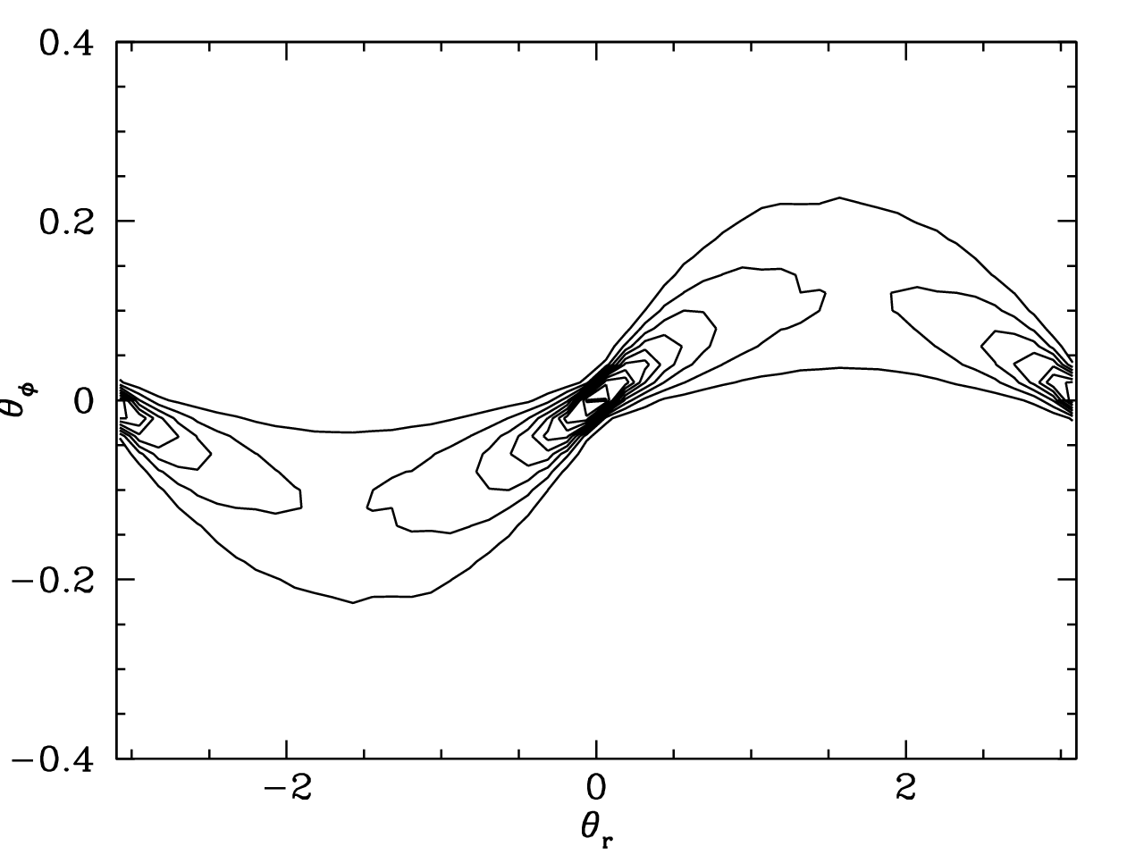
In Figure 5 I show density contours for the values of $\theta_{r}$ and $\theta_{\phi}$ taken from the phase-mixed model. There is a clear relationship between the two values, with $\theta_{\phi}\gtrsim 0$ for $\theta_{r}>0$, and $\theta_{\phi}\lesssim 0$ for $\theta_{r}<0$. There are extrema in $\theta_{\phi}$ at $\theta_{r}=\pm\pi/2$, and $\theta_{\phi}\approx 0$ for $\theta_{r}=0$ & $\pm\pi$. This is again due to the fact I am selecting stars from a very narrow range in $\phi$, and because of the relationship between $\theta_{r}$ and $\theta_{\phi}$ for a given orbit at a given point illustrated in Figures 1 and 2.

I now compare the phase-mixed model analysed in Section 4 to the stars in the Solar neighbourhood observed by the GCS. The GCS data are taken from the table produced by Holmberg et al. (2009), and I follow S10 in restricting the analysis to stars that have full 6D phase-space coordinates quoted, are at distances $\leq 200\,\mathrm{pc}$ from the Sun, and are not directly associated with the Hyades cluster. The distributions in angle space that I find are very similar to those found by S10, and the small differences are due to the different choices of Galactic potential and the use of torus-fitting as opposed to integrating orbits in the plane.

In Figure 6 I plot the distributions in $\theta_{r}+n\theta_{\phi}$ of the GCS stars (solid line) and those taken from the phase-mixed model (dotted line) for a series of integers $n$. Naively one would simply expect an OLR to produce a peak for some value of $n>0$, and an ILR to produce a peak for some value of $n<0$ (with the perturber being $|n|$-fold symmetric). The relationship between $\theta_{r}$ and $\theta_{\phi}$ due to selection effects produces a peak around $0$ in plots with $n<0$ and around $\pm\pi$ for $n>0$. ²² 2 The convention I use for these graphs means that for $n<0$ they are mirror images of the comparable figures in S10. This choice is made so that the features in the various plots can easily be “followed” from one to another as $n$ increases.

There are two main features in the angle distribution of the GCS data (besides those due to selection effects), one peak that lies at $\theta_{r}\sim-1.5$, and one that lies at $\theta_{r}\sim 2.2$. It is also noticeable that the peak at $0$ which appears in the model data for $n<0$ is offset to slightly lower values in the GCS data – this can be associated with the small peak in the $\theta_{r}$ distribution at $\theta_{r}\sim-0.4$.

Figure 7 shows the distribution of stars taken from the GCS data in the $v_{x},v_{y}$-plane (assuming the Solar velocity relative to the local standard of rest given in eq. 5) overlaid on the lines of constant $\theta_{r}$ and of constant $\theta_{\phi}$ (at the Sun’s position) as shown in Figure 2. This makes it easy to see which of the familiar features in the $v_{x},v_{y}$-plane correspond to which peaks in Figure 6. The peak at $\theta_{r}\sim-1.5$ is associated with the Hyades moving group, the peak at $\theta_{r}\sim 2.2$ is associated with the Sirius moving group and the peak at $\theta_{r}\sim-0.4$ is associated with the Pleiades moving group.

The peak at $\theta_{r}\sim-1.5$ clearly appears in all the plots shown in Figure 6, shifted to higher values for $n<0$ and to lower values for $n>0$. This peak is made up of almost the same set of stars in each plot. It is this feature that S10 identified as the signature of an ILR. It is clear from Figure 6 that these data are consistent with the stars that make up the peak at $\theta_{r}\sim-1.5$ being associated with any value of $n$ between $-4$ and $4$ (including non-integer values, and indeed for $|n|>4$ though these are not shown as selection effects create ever greater distortions). While S10 shows plots that are almost identical to the centre and bottom-left panels of Figure 6 (his fig. 4 upper panel and fig. 7 top panel, respectively), the peaks in these plots are misidentified as being primarily due to selection effects that S10 incorrectly claimed should result in high relative densities around $\theta_{r}=\pm\pi/2$.

The peak at $\theta_{r}\sim 2.2$ becomes a more clearly defined (and higher) peak for $n>0$ (shifted to higher values), and nearly disappears for $n<0$. It is also noticeable that the feature around $\theta_{r}\sim-1.5$ becomes more sharply peaked for $n<0$. This would seem to imply that the peak at $\theta_{r}\sim 2.2$ is associated with an OLR, and the peak at $\theta_{r}\sim-1.5$ is associated with an ILR, but this is not necessarily the case, both because of the selection effects discussed previously, and because of the other condition on resonant stars (eq. 2, see Section 6).

In Figure 8 I show a contour plot of the density in the $\theta_{r}$, $\theta_{\phi}$ plane of the selected stars from the GCS catalogue. The plots in Figure 6 are found from the distribution in angle space plotted in Figure 8 by marginalising it over straight lines, the gradient of which are determined by $n$. In Figure 8, lines corresponding to a few different values of $n$ are plotted, centred on the main overdensities, to guide the eye.

The distribution in the $\theta_{r},\theta_{\phi}$ plane seen in Figure 8 shows the same strong selection effects in $\theta$ illustrated by the phase-mixed model. These selection effects have a very strong effect on the overdensities associated with the Pleiades and Sirius moving groups, which drives them towards the observed correlation between $\theta_{r}$ and $\theta_{\phi}$ in the two different cases. The Hyades overdensity (around $\theta_{r}=-1.5$) is a less straightforward case. It is approximately triangular in the $\theta_{r},\theta_{\phi}$ plane, and lies either side of the expected minimum in $\theta_{\phi}$ at $\theta_{r}=-\pi/2$ (this minimum is seen in the phase-mixed model, Figure 5). The Hyades overdensity has increasing $\theta_{\phi}$ with increasing $\theta_{r}$ for $\theta_{r}>-\pi/2$, and with decreasing $\theta_{r}$ for $\theta_{r}<-\pi/2$ (Figure 8), and these are the directions one would expect the selection effects that affected the phase-mixed model to drive the observations. This selection effect is important, but it is not clear that it is enough to explain the observed shape, and in Section 6 I explore the distribution in angle space of models with a resonant component.

Figure 9 shows a contour plot of the GCS data distributed in polar coordinates with radial coordinate $a$ (the amplitude of radial motion under the epicycle approximation, eq. 3) and polar coordinate $\varphi=\theta_{r}-2\theta_{\phi}$ (left) or $\varphi=\theta_{r}+2\theta_{\phi}$ (right). These are comparable to the upper panel of S10’s fig. 8. In both cases one can see an overdensity at particular values of the polar coordinate, found (unsurprisingly) at the values of $\varphi$ one would anticipate given Figure 6. S10 only showed a version of the plot with $\varphi=\theta_{r}-2\theta_{\phi}$, finding that the plot for $\varphi=\theta_{r}+2\theta_{\phi}$ (i.e. the plot that would suggest an OLR) argued against the suggestion that the Hyades corresponded to an OLR, primarily because the overdensity in the $\varphi=\theta_{r}-2\theta_{\phi}$ plot appears to lie in a radial line out to larger $a$ in the figure, whereas in the $\varphi=\theta_{r}+2\theta_{\phi}$ plot it does not (Sellwood priv. comm.). This is not a particularly strong effect, but can be seen in Figure 9, and understanding it requires moving beyond a phase-mixed model.

Thus far in this study I have only considered two of the conditions on resonant stars – that they lie on or near lines of $l\theta_{r}+m\theta_{\phi}=const$ and that they must lie in the survey volume. To understand the expected distribution of resonant stars in a survey of the Solar neighbourhood, one must consider the combination of three different requirements on them:

• •

  They must have angle coordinates near to a given resonance line in angle (eq. 1).

• •

  They must have orbital frequencies (and thus actions) which place them near to a given resonance line in frequency (eq. 2).

• •

  They must lie within the survey volume (e.g. within $200\,\mathrm{pc}$ of the Sun).

Note that over the Galaxy as a whole, the requirement on $\theta$ only affects the distribution in $\theta$ and the requirement on $J$ only affects the distribution in $J$ -- the two distributions can be thought of as independent³³ 3 In practice they are not entirely independent – the resonant stars at the (say) higher values of $l\theta_{r}+m\theta_{\phi}$ about the resonance are probably there because they have the higher values of $l\Omega_{r}(\mbox{\boldmath{$J$}})+m\Omega_{\phi}(\mbox{\boldmath{$J$}})$. This effect is likely to have some impact, but is beyond the scope of this study. It is only because of the finite survey volume, and therefore the finite range of $\theta$ for which stars with for a given $J$ will be observed, that the $J$ condition significantly affects the observed $\theta$ distribution (and vice versa).

In Figure 10 I plot the density of the GCS stars as a function of $J_{\phi}$ and $J_{r}$. The density of stars in my phase-mixed model is also plotted, for comparison. For a given $J_{\phi}$ there is a minimum $J_{r}=J_{r,min}$ for stars to reach the Solar neighbourhood, which can be thought of as a minimum epicyclic amplitude for a given guiding centre radius⁴⁴ 4 For a given $J_{\phi}$, the value of $J_{r,min}$ is in fact dependent on $J_{z}$, with increasing $J_{z}$ generally causing a decrease in $J_{r,min}$ if $J_{\phi}<J_{\phi,SN}$, and an increase in $J_{r,min}$ if $J_{\phi}>J_{\phi,SN}$, where $J_{\phi,SN}$ is the angular momentum of a circular orbit that passes through the Solar neighbourhood. This effect is small for the stars considered here as they have $J_{z}\ll J_{\phi}$.. This is the cause of the near-parabolic lower boundary seen in Figure 10. The Pleiades and Sirius moving groups can be clearly seen as small overdensities in this plot. The Hyades moving group is seen as a rather more spread out overdensity at a range of $J_{r}$, around $J_{\phi}=0.97J_{\phi,0}$, tending towards slightly lower $J_{\phi}$ with increasing $J_{r}$.

The dotted and dashed lines in Figure 10 are 2:1 OLR and ILR lines respectively, these are lines along which $2\Omega_{\phi}(\mbox{\boldmath{$J$}})+\Omega_{r}(\mbox{\boldmath{$J$}})=2\Omega_{p}$ and $2\Omega_{\phi}(\mbox{\boldmath{$J$}})-\Omega_{r}(\mbox{\boldmath{$J$}})=2\Omega_{p}$ respectively, for different values of $\Omega_{p}$, the perturber pattern speed, chosen such that the resonance lines reach $J_{r}=0$ at $J_{\phi}=0.9,\,1$, or $1.1J_{\phi,0}$. Changing the value of $\Omega_{p}$ moves the resonance lines in $J_{\phi}$, but does not significantly alter their gradient in this range of $J$. The Hyades overdensity seems to lie around a Lindblad resonance line, but this could be either an OLR or ILR line – it was this fact which lead S10 to claim this was an Lindblad resonance, but that one needed to investigate the distribution in angle to determine which one. Other resonances – the 3:1 or 4:1 OLR or ILR lines – would appear very similar on Figure 10, though the 2:1 ILR line is the furthest from the vertical. It is also worth noting that the slope of the various resonance lines is sensitive to the Galactic potential – in a logarithmic potential (of the kind used by S10), the gradients of the 2:1 OLR and ILR lines in this part of $J$-space are nearly identical. It may be possible to use the slope of resonance lines in action space to provide information about the Galactic potential by comparing them to observed dynamical substructure, but that is beyond the scope of this study.

To explore the expected distribution of stars in the Solar neighbourhood associated with a resonance, I consider a df related to the phase-mixed df used previously, adjusted to include a resonant component:

where $f_{0}$ is the distribution function described in Section 3, $C$ is a constant chosen such that the resonant component contributes $8$ percent of the stars observed in the Solar neighbourhood, and

$J_{\phi,res}$ is a function of $J_{r}$ and is chosen such that $l\Omega_{r}(J_{r},J_{\phi,res})+m\Omega_{\phi}(J_{r},J_{\phi,res})=const$, for $J_{z}=0$, and $\theta_{r,res}$ is a function of $\theta_{\phi}$ and is chosen such that $l\theta_{r,res}+m\theta_{\phi}=const$. The values $\Delta_{J,res}$ and $\Delta_{\theta,res}$ give the width of the resonance peak around the exact resonance lines in $J_{\phi}$ and $\theta_{r}$, respectively. One could, equally, describe the width in action or angle in terms of a spread in $J_{r}$ or $\theta_{\phi}$ respectively, but for convenience I have chosen to describe it in terms of the coordinates with the greater ranges of values in these data. The width $\Delta_{J,res}$ is effectively a width in frequency about the pattern speed of the perturber. In the toy models I show here I take $\Delta_{J,res}=0.01J_{\phi,0}$, $\Delta_{\theta,res}=0.3$.

I consider two toy models, each designed to produce models with an overdensity in phase-space in a similar volume to that where the Hyades moving group is found (but not tuned to produce a best fit), one corresponding to an OLR ($l=1$, $m=2$) and one corresponding to an ILR ($l=-1$, $m=2$). For the OLR model, I take $\theta_{r,res}+2\theta_{\phi}=-1.9$, and for the ILR model $-\theta_{r,res}+2\theta_{\phi}=1.3$. In the OLR case I take $J_{\phi,res}(J_{r}=0)=0.975J_{\phi,0}$, and in the ILR case $J_{\phi,res}(J_{r}=0)=0.985J_{\phi,0}$.

Figure 11 shows contour plots of the density in the $\theta_{r}$, $\theta_{\phi}$ plane of the OLR and ILR models, and plots of $\theta_{r}+n\theta_{\phi}$ (as in Figure 6) restricted to $n=\pm 2$ in the interests of brevity. Both the ILR and OLR models reproduce some of the features of the Hyades overdensity. In both cases the overdensity in angle space is somewhat triangular in shape, like the Hyades overdensity, rather than following a single line as one would expect if only the condition on angle (eq. 1) was relevant. In both cases the overdensity in angle is strong for the two cases $n=\pm 2$, as well for other values of $n$ (not shown).

In an effort to explain the structure of the overdensity in the $\theta_{r}$, $\theta_{\phi}$ plane, the upper panels of Figure 11 also show the lines $\theta_{r}=\theta_{r,res}$ for the two models, and lines corresponding to the condition on $J$. The latter are found by taking the condition that $J_{\phi}=J_{\phi,res}(J_{r})$ (or $J_{\phi}=J_{\phi,res}\pm\Delta_{J,res}$ or $J_{\phi}=J_{\phi,res}\pm 2\Delta_{J,res}$) and determining the two possible values of $\theta$ that a star with these actions would have at the Sun’s position – in the relevant part of phase space, lower values of $J_{r}$ correspond to smaller (i.e. closer to zero) values of $\theta_{\phi}$. This gives a sense of the two competing effects which (in addition to the general selection effects illustrated in Figure 5) determine the shape of the overdensity in angle space, but it is important to also consider the effect of the finite volume surveyed on the constraint applied by the condition on $J$, i.e. how close to the dotted lines in Figure 11 stars must actually lie.

A star with a given value of $J$ which lies within $200\,\mathrm{pc}$ of the Sun will have a value $\theta_{\phi}$ which lies within $\sim 0.02$ of the value for a star at the Sun, while the range of possible values of $\theta_{r}$ is typically larger, and increases with decreasing $J_{r}$ (and thus, in the overdensity considered, with decreasing $\theta_{\phi}$). This latter point can be understood by considering a star in the epicycle approximation. As $J_{r}\rightarrow 0$ the epicycle shrinks to negligible size, so the star can be at any point on the epicycle (therefore any $\theta_{r}$) and still be within the survey volume if the value of $\theta_{\phi}$ is one that places it there. As $J_{r}$ increases, and the epicycle increases in size, the fraction of the epicycle (i.e. the range in $\theta_{r}$) that corresponds to stars that enter the survey volume decreases.

Figure 12 shows polar plots, analogous to those in Figure 9, each labeled with which model they represent and what was used as the polar angle $\varphi$ (the radial coordinate, as before, is always radial epicycle amplitude $a$). In each case I again plot the lines corresponding to $\theta_{r}=\theta_{r,res}(\theta_{\phi})$ and $J_{\phi}=J_{\phi,res}(J_{r})$, evaluated at the Sun’s position. Once again, it is clear that both resonant conditions are important on the distribution in these plots, so the overdensity seen will be distorted away from $\theta_{r}+n\theta_{\phi}=const$ even if the model has $\theta_{r,res}+n\theta_{\phi}=const$ as a constraint, providing there is a non-negligible width around the resonance in $\theta$.

Note that as $J_{r}$ increases (and the size of the epicycle increases), the condition on $J$ becomes more restrictive in $\theta$ for the reason discussed above. Therefore this condition becomes increasingly dominant on the observed overdensity. This can be seen in Figure 12 as the outer contours show that the overdensity appears to follow the dotted line corresponding to $J_{\phi}=J_{\phi,res}(J_{r})$ at large $J_{r}$. For both of the models this means that the contours seem to show an overdensity that lies around a value of $\theta_{r}-2\theta_{\phi}$ that is approximately constant with increasing $J_{r}$, while lying around a value of $\theta_{r}+2\theta_{\phi}$ that varies with increasing $J_{r}$. This provides a natural explanation for the slight curvature as $J_{r}$ increases of the overdensity associated with the Hyades moving group in the equivalent plot for the GCS stars (Figure 9) – for overdensities produced by either an OLR or ILR, this curvature is seen as a result of the selection effects and the constraint in $J$.

I have explored models with resonances at other frequency ratios (and thus with different relationships between $\theta_{r}$ and $\theta_{\phi}$), and found that it is possible to produce overdensities in $\theta$ that are qualitatively very similar to those shown here. While it may be possible to tell one from another for given observations (such as those of the Hyades) it is certainly a very complicated task, and one that will require careful modelling and analysis.

In this paper I have re-examined the distribution of stars in the Solar neighbourhood in angle coordinates following the claim by S10 that the Hyades moving group is related to an ILR. Using a dynamical “torus” model I showed the significant impact of selection effects associated with surveying a finite (small) volume upon the distribution of stars in angle coordinates taken from a phase-mixed model. Using models which contain resonant components in addition to a phase-mixed background I have demonstrated the important effects that the distribution of resonant stars in action have on the observed distribution in angle (again because of selection effects).

The distribution of the stars associated with the Hyades moving group in action (Figure 10) indicates that it is associated with some resonance between the radial oscillations and the azimuthal motion (i.e. follows a relation of the form of $l\Omega_{r}+m\Omega_{\phi}$). It is also clear that the stars which make up the resonant component are constrained in $\theta$ in some way, otherwise there would be an overdensity at $\theta_{r}\sim 1.5$ as well as $\theta_{r}\sim-1.5$. However, it is very difficult to determine what the values of $l$ and $m$ are, and thus which resonance is responsible. In action space the lines $l\Omega_{r}(\mbox{\boldmath{$J$}})+m\Omega_{\phi}(\mbox{\boldmath{$J$}})=const$ are very similar, in the relevant range of $J$, for different values of $l$ and $m$, and are sensitive to choice of the Galactic potential. The approach taken by S10, of looking for overdensities in the statistic $l\theta_{r}+m\theta_{\phi}$, is also flawed because of the selection effects that have important influences on the distribution in $\theta$. I find that, contrary to the conclusions of S10, it not clear that the Hyades moving group is the result of an inner Lindblad resonance.

It may be possible to use careful modeling and analysis, which takes into account selection effects and the distributions in $\theta$ and $J$ simultaneously, to determine what type of resonance is responsible for the Hyades moving group from these data. However this task is made even more difficult by uncertainty about the Galactic potential which significantly affects the gradient of resonance lines in action space.

It seems likely the problems of selection effects in studies of this kind will prove extremely challenging, if not intractable, while we are dealing with survey volumes corresponding to the relatively small radii ($\sim 200\,\mathrm{pc}$) associated with the GCS. To go beyond this with similar accuracy (i.e. $\sim 1\,\mathrm{km\,s}^{-1}$ velocity uncertainty) requires distance and proper measurements more accurate than those currently available – the RAVE and SDSS data used by Hahn et al. (2011) has significantly larger uncertainties even though they select stars which lie in the same volume as the GCS stars. Gaia (Perryman et al., 2001) is expected to produce 3-dimensional velocity measurements accurate to $\sim 1\,\mathrm{km\,s}^{-1}$ for some stars up to $\sim 3\,\mathrm{kpc}$ from the Sun, corresponding to a range in Galactocentric $\phi$ of order $0.7$ radians. This will dramatically reduce the impact of selection effects on the observed distributions in angle-action coordinates, and should make it relatively straightforward to pick out structures in angle space that are unambiguously of the kind predicted by S10. This process is likely to both be guided by and affect the determination of the gravitational potential of the Galaxy (an essential product of the Gaia mission).

Throughout this study I have assumed that the uncertainties on the positions and velocities of the stars observed by the GCS can be ignored, because they are too small to have any significant effect. It is worth noting that the relationship between the uncertainty in $\mbox{\boldmath{$x$}},\mbox{\boldmath{$v$}}$ and that in $\mbox{\boldmath$\theta$},\mbox{\boldmath{$J$}}$ is not entirely straightforward, and that a small uncertainty in velocity does not necessarily correspond to a small uncertainty in $\theta$. As inspection of Figure 2 suggests, the relationship between an uncertainty in velocity and that in $\theta_{r}$ is heavily dependent on $J_{r}$, with smaller $J_{r}$ corresponding to a greater uncertainty in $\theta_{r}$ for given uncertainty in $v$. Indeed as $J_{r}\rightarrow 0$ a negligible uncertainty in $v$ corresponds to an uncertainty of $2\pi$ in $\theta_{r}$. The Hyades overdensity does not extend to $J_{r}=0$ (as can be seen in Figure 7), so the assumption that the uncertainty in $\theta_{r}$ can be ignored is reasonable for this study. However, future efforts to understand resonances of this type is likely to require appropriate treatment of these uncertainties.

I thank members of the Oxford dynamics group for helpful input, especially James Binney for careful reading of an early draft of this paper. I am also grateful to Jerry Sellwood for a very helpful discussion which provoked the work described in Section 6. This work is supported by a grant from the Science and Technology Facilities Council.

References

- Abazajian et al. (2009) Abazajian K. N., Adelman-McCarthy J. K., Agüeros M. A., et al., 2009, ApJS, 182, 543
- Binney (2010) Binney J., 2010, MNRAS, 401, 2318
- Binney & McMillan (2011) Binney J., McMillan P., 2011, MNRAS, 413, 1889
- Binney & Tremaine (2008) Binney J., Tremaine S., 2008, Galactic Dynamics: Second Edition. Princeton University Press
- Dehnen (1998) Dehnen W., 1998, AJ, 115, 2384
- ESA (1997) ESA, 1997, VizieR Online Data Catalog, 1239, 0
- Famaey et al. (2005) Famaey B., Jorissen A., Luri X., Mayor M., Udry S., Dejonghe H., Turon C., 2005, A&A, 430, 165
- Hahn et al. (2011) Hahn C. H., Sellwood J. A., Pryor C., 2011, arXiv:1102.4626
- Holmberg et al. (2009) Holmberg J., Nordström B., Andersen J., 2009, A&A, 501, 941
- McMillan (2011) McMillan P. J., 2011, MNRAS, 414, 2446
- McMillan & Binney (2008) McMillan P. J., Binney J. J., 2008, MNRAS, 390, 429
- Navarro et al. (1996) Navarro J. F., Frenk C. S., White S. D. M., 1996, ApJ, 462, 563
- Perryman et al. (2001) Perryman M. A. C., de Boer K. S., Gilmore G., Høg E., Lattanzi M. G., Lindegren L., Luri X., Mignard F., Pace O., de Zeeuw P. T., 2001, A&A, 369, 339
- Schönrich et al. (2010) Schönrich R., Binney J., Dehnen W., 2010, MNRAS, 403, 1829
- Sellwood (2010) Sellwood J. A., 2010, MNRAS, 409, 145
- Steinmetz et al. (2006) Steinmetz M., Zwitter T., Siebert A., et al., 2006, AJ, 132, 1645